
We denote by \(\mathcal{A}\) the family of all analytic functions defined in the unit disk \(\mathbb{D} =\{z \in \mathbb{C} : |z| < 1\}\) that admit a Taylor–Maclaurin series expansion of the form \[ f(z) = z + \sum\limits_{n=2}^{\infty} a_n z^n, \quad z \in \mathbb{D}. \tag{1} \]
Let \(\mathcal{S}\) stand for the subclass of \(\mathcal{A}\) consisting of functions that are univalent in \(\mathbb{D}\). We first recall two well-known subclasses of \(\mathcal{A}\) that provide the geometric setting for the present investigation. Their standard analytic characterizations are given below; further details can be found in [1]. \[ \mathcal{S}^*=\{ f\in \mathcal{A}: \mathrm{Re}\Big( \frac{zf'(z)}{f(z)}\Big)>0, \quad (z\in \mathbb{D})\}. \tag{2} \]
The corresponding convex class is defined by \[ \mathcal{C}=\{ f\in \mathcal{A}: \mathrm{Re}\Big( \frac{(zf'(z))’}{f'(z)}\Big)>0, \quad (z\in \mathbb{D})\}. \tag{3} \]
Functions analytic in \(\mathbb{D}\) that satisfy the conditions in (2) and (3) are called starlike and convex functions, respectively. A function \(f \in \mathcal{A}\) is said to be starlike of reciprocal order \(\alpha\), \(\alpha \in [0,1)\), denoted \(f \in \mathcal{S}_r^*(\alpha)\) [2], if \[ \mathrm{Re}\left\{ \dfrac{f(z)}{zf'(z)} \right\} > \alpha, \quad z \in \mathbb{D}. \tag{4} \]
It is a classical result that any starlike function of reciprocal order \(0\) is starlike. More generally, for every \(\alpha \in [0,1)\), starlikeness of reciprocal order \(\alpha\) implies starlikeness, and consequently univalence in \(\mathbb{D}\) [3]. Several researchers have investigated problems related to the classes \(\mathcal{S}_r^*(\alpha)\); see, for instance, [2,3]. The present investigation uses a real parameter \(\vartheta\), with \(0\leq\vartheta\leq1\), to connect the starlike and convex endpoint conditions. The associated differential operator \(\mathcal{L}_{\vartheta}\) plays a fundamental role in defining the proposed class and in interpreting its coefficient relations. For the transformed function \[ \mathcal{L}_{\vartheta}f(z) =(1-\vartheta)f(z)+\vartheta zf'(z), \] differentiation gives \[ (\mathcal{L}_{\vartheta}f(z))’ =(1-\vartheta)f'(z) +\vartheta\left(f'(z)+zf”(z)\right) =f'(z)+\vartheta zf”(z). \]
Consequently, \[ z(\mathcal{L}_{\vartheta}f(z))’ =zf'(z)+\vartheta z^2f”(z), \] and hence \[ \frac{zf'(z)+\vartheta z^2f”(z)} {(1-\vartheta)f(z)+\vartheta zf'(z)} = \frac{z(\mathcal{L}_{\vartheta}f(z))’} {\mathcal{L}_{\vartheta}f(z)}. \]
Thus, the differential expression appearing in the definition of the new class can be interpreted as the logarithmic derivative associated with the transformed function \(\mathcal{L}_{\vartheta}f\). This identity establishes the structural relationship between the newly defined class and the corresponding starlike and convex classes, \(\mathcal{S}^*\) and \(\mathcal{C}\), at the respective parameter endpoints.
Recall that if \(F\) and \(G\) are analytic in \(\mathbb{D}\), then \(F\) is subordinate to \(G\), written \(F(z) \prec G(z)\) [4], provided there exists a Schwarz function \(w\) in \(\mathbb{D}\) satisfying \(w(0) = 0\) and \(|w(z)| < 1\) such that \(F(z) = G(w(z))\) for all \(z \in \mathbb{D}\). As a consequence of the Schwarz lemma, the relation \(F(z) \prec G(z)\) yields \(F(\mathbb{D}) \subset G(\mathbb{D})\). When \(G\) is univalent in \(\mathbb{D}\), we have the equivalence \[ F(z) \prec G(z) \iff F(0) = G(0) \quad \text{and} \quad F(\mathbb{D}) \subset G(\mathbb{D}). \]
In [5], the authors defined the class \(\mathcal{S}_{4L}^*\) to consist of functions \(f \in \mathcal{A}\) such that \[ \dfrac{zf'(z)}{f(z)} \prec 1 + \dfrac{5z}{6} + \dfrac{z^5}{6} , \quad z \in \mathbb{D}. \tag{5} \]
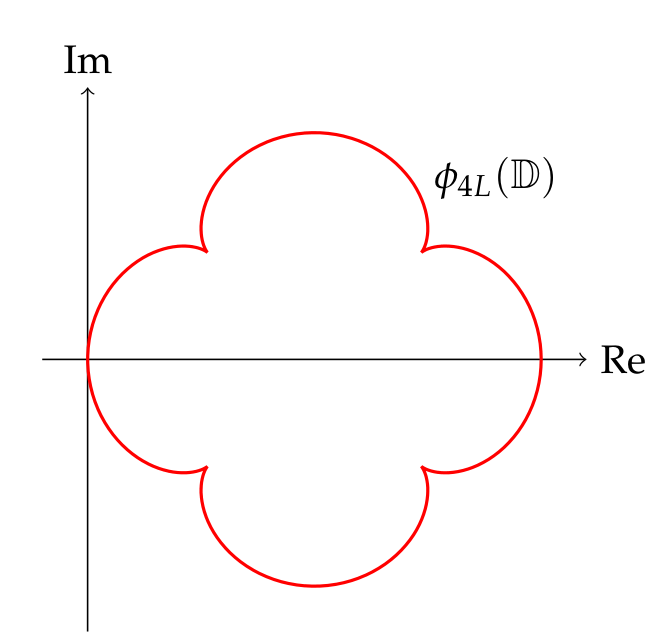
Coefficient bounds and differential subordinations for classes associated with starlike functions were investigated in [6]. The general framework developed by Ma and Minda [7] provides an important context for defining subclasses through a prescribed analytic mapping. Gandhi [8] subsequently studied radius problems involving a three-leaf function and convex combinations of starlike functions. More recent investigations [9–11] define and examine several subclasses through subordination to a four-leaf function. The boundary curve associated with this mapping is illustrated in Figure 1, which plots its real and imaginary components on the unit circle. The defining function is \[ \phi_{4L}(z) =1 + \dfrac{5}{6}z + \dfrac{1}{6}z^5, \quad z \in \mathbb{D}. \tag{6} \]
The geometry of the four-leaf image domain specifies the range used in the subordination condition. Its coefficients and boundary structure distinguish this choice from other generating functions used in Ma–Minda-type subclasses. The subsequent coefficient calculations therefore retain the explicit form of the four-leaf mapping throughout the argument.
Using this four-leaf function and the principle of subordination, we introduce the following subclass of \(\mathcal{A}\).
Definition 1. A function \(f\in \mathcal{A}\) is said to belong to the class \(\mathfrak{M}(\vartheta,\phi_{4L})\) if \[ \dfrac{z f^{\prime}(z)+\vartheta z^2 f^{\prime \prime}(z)}{(1-\vartheta) f(z)+\vartheta z f^{\prime}(z)}\prec \phi_{4L}(z), \tag{7} \] where \(0\leq\vartheta\leq1\) and \(\phi_{4L}\) is the four-leaf function defined in (6). The quotient at the origin is understood through its analytic continuation, whose value is 1.
For convenience, we denote by \(\mathfrak{M}(\vartheta,\phi_{4L})\) the class of functions satisfying (7).
Remark 1. The two endpoint values of the parameter give the following notable specializations of the class \(\mathfrak{M}(\vartheta,\phi_{4L})\): \[ \begin{aligned} \text{(i) For } \vartheta=1 ~\text{in}~ \text{(7)} \quad \mathfrak{M}(1,\phi_{4L}) &:=\mathcal{K}_{4L}= \left\{f\in\mathcal{A}:\ \dfrac{(zf'(z))’}{f'(z)}\prec\phi_{4L}(z)\right\}, \end{aligned} \tag{8} \]\[ \begin{aligned} \text{(ii) For } \vartheta=0 ~\text{in}~\text{(7)} \quad \mathfrak{M}(0,\phi_{4L}) &:=\mathcal{S}_{4L}= \left\{f\in\mathcal{A}:\ \dfrac{zf'(z)}{f(z)}\prec \phi_{4L}(z)\right\}, \end{aligned} \tag{9} \] Here the four-leaf function \(\phi_{4L}\) is given by (6), and the subordination conditions hold for every \(z\in\mathbb{D}\).
The Alexander relation between convex and starlike functions gives the equivalence \[ f \in \mathcal{K}_{4L} \iff z f'(z) \in \mathcal{S}_{4L}^*, \] provided that \(f \in \mathcal{A}\). Here \(\mathcal{S}_{4L}\) and \(\mathcal{S}_{4L}^{*}\) denote the same starlike four-leaf class; this convention connects the endpoint notation with the earlier definition. The classes introduced above generalize several previously studied subclasses associated with special analytic mappings such as nephroid, limaçon, and trigonometric domains. The use of the four-leaf mapping \(\phi_{4L}\) imposes additional geometric restrictions on the image domain and leads to new coefficient estimates and related functional inequalities.
Remark 2. The function \(\phi_{4L}(z)=1+\dfrac56 z+\dfrac16 z^5\) maps the unit disk \(\mathbb D\) onto the bounded four-leaf domain \(\phi_{4L}(\mathbb D)\), which is starlike with respect to the point \(w_0=1\).
Remark 3. The class \(\mathfrak{M}(\vartheta,\phi_{4L})\) is nonempty for every parameter value considered here. This can be verified directly from the defining quotient, without requiring a separate construction of a polynomial or rational family. In particular, the constant Schwarz function \(w(z)=0\) provides the subordination needed for the normalized identity function. The normalized identity function gives an immediate example: \[ f(z)=z \quad\Longrightarrow\quad \dfrac{z f'(z)+\vartheta z^{2}f”(z)} {(1-\vartheta)f(z)+\vartheta zf'(z)} =1=\phi_{4L}(0). \]
It follows that the class \(\mathfrak{M}(\vartheta,\phi_{4L})\) is nonempty.
The proofs use coefficient inequalities for analytic functions with positive real part. The normalized Carathéodory class is denoted by \(\mathcal{P}\), and the coefficients of its members are written as \(c_k\). This notation will be retained when a Schwarz function is transformed into a positive-real-part function in the subsequent proofs. The normalization and positivity requirements are stated explicitly below. A function \(p\) is said to belong to the class \(\mathcal{P}\) of Carathéodory functions [12,13] if and only if it admits the series representation \[ p(z) = 1 + \sum\limits_{k=1}^{\infty} c_k z^k,\quad z \in \mathbb{D}, \tag{10} \] and satisfies \(\mathrm{Re}\,p(z) > 0\) for all \(z \in \mathbb{D}\).
The main objective of this paper is to investigate coefficient estimates, Fekete–Szegő inequalities, logarithmic coefficients, inverse coefficients, inverse logarithmic coefficients and quotient coefficient estimates for functions belonging to the class \(\mathfrak{M}(\vartheta,\phi_{4L})\).
Lemma 1. Let \(p \in \mathcal{P}\) be given by (10). Then the following coefficient inequalities hold, with the parameter restrictions stated in each part:
(i) For every \(n \ge 1\), \[ |c_n| \le 2. \tag{11} \]
Equality in (11) holds for all \(n \ge 1\) if and only if \(p(z) = \dfrac{1 + \alpha z}{1 – \alpha z}\) with \(|\alpha| = 1\).
(ii) Furthermore, if \(\aleph \in \mathbb{C}\), then \[ |c_{n+k} – \aleph c_n c_k| \le 2 \max\{1, |2 \aleph – 1|\}, \tag{12} \] for all \(n, k \ge 1\). If \(0 < \aleph < 1\), the estimate (12) is sharp for \(p(z) = \dfrac{1 + z^{n+k}}{1 – z^{n+k}}\). For all other cases, equality is attained by \(p(z) = \dfrac{1 + z}{1 – z}\).
(iii) In addition, if \(B \in [0,1]\) and \(B(2B – 1) \le D \le B\), then \[ \left |c_3 – 2B c_1 c_2 + D c_1^3\right | \le 2. \tag{13} \]
Inequality (11) is the classical coefficient estimate associated with Carathéodory’s lemma [12]. A standard account, including the corresponding equality discussion, can also be found in Duren’s treatment of functions with positive real part [1, p. 41].
Inequality (12) corresponds to Theorem 1 of [14], while the sharpness for \(0 < \aleph < 1\) is given in [15, Lemma 2.3]. The particular case \(\aleph = 1\) was proved in a more general setting for \(p(0) = c_0\) in [16, Lemma 1, p. 546]. Inequality (13) is established in [17, Lemma 3, p. 66].
The following theorem provides upper bounds for the first three nontrivial Taylor coefficients, namely \(|a_2|\), \(|a_3|\), and \(|a_4|\), of functions belonging to \(\mathfrak{M}(\vartheta,\phi_{4L})\). The dependence on the parameter is displayed explicitly in each estimate.
Theorem 1. If the function \(f \in \mathfrak{M}(\vartheta,\phi_{4L})\) is given by (1), then for \(\vartheta\in[0,1]~,\) \[ \begin{aligned} |a_{2}| \leq& \dfrac{5}{6(1+\vartheta)}, \end{aligned} \tag{14} \]\[ \begin{aligned} |a_{3}|\leq& \dfrac{5}{12(1+2 \vartheta)}, \end{aligned} \tag{15} \]\[ \begin{aligned} |a_{4}|\leq & \dfrac{5}{18(1+3 \vartheta)}. \end{aligned} \tag{16} \]
Proof. Suppose that \(f\in \mathfrak{M}(\vartheta,\phi_{4L})\) has the form (1). Then there exists a function \(w\) analytic in \(\mathbb{D}\) with \(w(0)=0\) and \(|w(z)|<1\), \(z \in\mathbb{D}\), satisfying \[ \dfrac{z f^{\prime}(z)+\vartheta z^2 f^{\prime \prime}(z)}{(1-\vartheta) f(z)+\vartheta z f^{\prime}(z)}= \phi_{4L}(w(z)),\qquad z\in\mathbb{D}. \tag{17} \]
Expanding the quotient into a power series, we obtain
\[ \begin{aligned} \frac{z f^{\prime}(z)+\vartheta z^2 f^{\prime\prime}(z)} {(1-\vartheta)f(z)+\vartheta z f^{\prime}(z)} &=1+a_2(1+\vartheta)z +\Big[ 2a_3(1+2\vartheta) -a_2^2(1+\vartheta)^2 \Big]z^2 \ &\quad +\Big[ 3a_4(1+3\vartheta) -3a_2a_3(1+\vartheta)(1+2\vartheta) +a_2^3(1+\vartheta)^3 \Big]z^3 \ &\quad +\Big[ 4a_5(1+4\vartheta) -4a_2a_4(1+\vartheta)(1+3\vartheta) -2a_3^2(1+2\vartheta)^2 \ &\ \ \ \ \ +4a_2^2a_3(1+\vartheta)^2(1+2\vartheta) -a_2^4(1+\vartheta)^4 \Big]z^4 +\cdots, \qquad z\in\mathbb{D}. \end{aligned} \tag{18} \]
Suppose that the function \(c\) is defined by \[ c(z):=\frac{1+w(z)}{1-w(z)} =1+\sum\limits_{n=1}^{\infty}c_nz^n, \qquad z\in\mathbb{D}. \tag{19} \]
Since \(|w(z)|<1\) in \(\mathbb{D}\), it follows that \(c\in\mathcal{P}\).
A simple computation gives \[ w(z)=\dfrac{c(z)-1}{c(z)+1} =\dfrac12 c_1 z +\dfrac12\left(c_2-\dfrac12 c_1^2\right)z^2 +\dfrac12\left(c_3-c_1c_2+\dfrac14 c_1^3\right)z^3+\cdots, \tag{20} \] Substituting the power-series expansion in (20) into the right-hand side of (17) and collecting equal powers of \(z\) gives \[ \begin{aligned} \dfrac{z f^{\prime}(z)+\vartheta z^2 f^{\prime \prime}(z)}{(1-\vartheta) f(z)+z\vartheta f^{\prime}(z)}= & 1+\dfrac{5}{12} c_1 z+\left(\dfrac{5}{12} c_2-\dfrac{5}{24} c_1^2\right) z^2+\left(\dfrac{5}{12} c_3-\dfrac{5}{12} c_1 c_2+\dfrac{5}{48} c_1^3\right) z^3 \ & +\left(\dfrac{5}{12} c_4-\dfrac{5}{12} c_1 c_3-\dfrac{5}{24} c_2^2+\dfrac{5}{16} c_1^2 c_2-\dfrac{5}{96} c_1^4\right) z^4 + \cdots. \end{aligned} \tag{21} \]
Comparing the coefficients of \(z\), \(z^2\), and \(z^3\) in (18) and (21), we obtain the following three identities: \[ \begin{aligned} a_{2}=& \dfrac{5}{12(1+\vartheta)} c_1, \end{aligned} \tag{22} \]\[ \begin{aligned} a_{3}=&\dfrac{5}{24(1+2 \vartheta)}c_2-\dfrac{5}{288(1+2 \vartheta)} c_1^2 , \end{aligned} \tag{23} \]\[ \begin{aligned} a_{4}=&\dfrac{5}{36(1+3 \vartheta)} c_3-\dfrac{5}{96(1+3 \vartheta)} c_1 c_2+\dfrac{35}{10368(1+3 \vartheta)} c_1^3 . \end{aligned} \tag{24} \]
Applying the coefficient estimate (11) to (22) immediately yields the bound stated in (14).
Equation (23) can be rewritten in the form \[ |a_3|=\dfrac{5}{24(1+2\vartheta)}\left|c_2-\dfrac{1}{12}c_1^2\right|~, \quad \vartheta \in [0,1]. \tag{25} \]
Applying inequality (12) to the expression in (25) with \(n=k=1\), \(\aleph=\dfrac{1}{12}\), we get \[ |a_3|\leq\dfrac{5}{12(1+2\vartheta)}\qquad\vartheta \in [0,1], \]
Similarly, factoring the coefficient expression in (24) gives \[ a_{4}=&\dfrac{5}{36(1+3 \vartheta)} \left[c_3-\dfrac{3}{8} c_1 c_2+\dfrac{7}{288} c_1^3\right]. \]
Comparing the right-hand side of the above relation with inequality (13) using the conditions \(0 \leq B \leq 1,~ B(2B-1)\leq D \leq B,~\vartheta \in [0,1]\) and taking \(B=\dfrac{3}{{16}}, D=\dfrac{7}{288}\) gives \[ |a_{4}|\leq \dfrac{5}{18(1+3 \vartheta)}, \quad\quad \vartheta \in[0,1]. \]\(\square\)
Remark 4. The obtained estimates are sharp. Equality in the estimate for \(|a_2|\) is attained for the extremal Carathéodory function \[ p_1(z)=\frac{1+e^{i\theta}z}{1-e^{i\theta}z}, \qquad \theta\in\mathbb{R}, \] or, in particular, for \(p_1(z)=(1+z)/(1-z)\). For the estimate of \(|a_3|\), equality is attained for \[ p_2(z)=\frac{1+e^{i\theta}z^2}{1-e^{i\theta}z^2}, \qquad \theta\in\mathbb{R}, \] whereas the estimate of \(|a_4|\) is attained for \[ p_3(z)=\frac{1+e^{i\theta}z^3}{1-e^{i\theta}z^3}, \qquad \theta\in\mathbb{R}. \]
These extremal Carathéodory functions satisfy (11), and the corresponding functions \(f\), generated through the defining subordination relation associated with the four-leaf mapping \(\phi_{4L}(z)\), belong to the proposed class and attain equality in the respective estimates. Hence, the stated coefficient bounds are sharp.
Setting \(\vartheta=0\) and \(\vartheta=1\) in Theorem 1, we obtain the following corollary, which records the two endpoint cases separately.
Corollary 1.
(i) If the function \(f \in \mathcal{S}_{4L}\) is given by (1), then \[ |a_2| \le \dfrac{5}{6}, \quad |a_3| \le \dfrac{5}{12}, \quad |a_4| \le \dfrac{5}{18}. \]
(ii) If the function \(f \in \mathcal{K}_{4L}\) is given by (1), then \[ |a_2| \le \dfrac{5}{12}, \quad |a_3| \le \dfrac{5}{36}, \quad |a_4| \le \dfrac{5}{72}. \]
Fekete and Szegő [18] established the following classical extremal relation for the normalized univalent class: \[ \max\left\{|a_3 – \aleph a_2^2| : f \in {\mathcal{S}}\right\} = 1 + 2e^{-\left(\dfrac{2 \aleph}{1- \aleph}\right)}, \; \aleph \in [0,1). \]
The following theorem gives the corresponding Fekete–Szegő inequality for the class \(\mathfrak{M}(\vartheta,\phi_{4L})\), with an arbitrary complex parameter in the coefficient functional.
Theorem 2. If the function \(f \in \mathfrak{M}(\vartheta,\phi_{4L})\) is given by (1) and \(\aleph\in \mathbb{C}\), then \[ \left| a_3 – \aleph a_2^2 \right|\le\dfrac{5}{12(1+2\vartheta)} \max \left\{1,\dfrac{5}{6}\left|\dfrac{-\vartheta^2+2\vartheta(2 \aleph-1)+2 \aleph-1}{(1+\vartheta)^2}\right|\right\}. \tag{26} \]
Proof. Let \(f\in\mathfrak{M}(\vartheta,\phi_{4L})\) have the expansion (1). Using the coefficient identities (22) and (23) established in the preceding proof gives \[ a_3- \aleph a_2^2 =\dfrac{5}{24(1+2\vartheta)}\left[c_2-\left(\dfrac{1}{12}+\dfrac{5(1+2\vartheta)}{6(1+\vartheta)^2} \aleph\right)c_1^2\right]. \tag{27} \]
Now consider \[ \begin{aligned} \lambda(\aleph, \vartheta) & =\dfrac{5(1+2 \vartheta) \aleph}{6(1+\vartheta)^2}+\dfrac{1}{12} . \end{aligned} \]
This definition gives the relation \[ |2\lambda(\aleph, \vartheta)-1|\leq \dfrac{5}{6}\left| \dfrac{-\vartheta^2+2 \vartheta(2\aleph-1)+2\aleph-1}{(1+\vartheta)^2}\right|. \]
Remark 5. The Fekete–Szegő functional obtained above is sharp since the proof relies on the sharp coefficient inequality for functions in the Carathéodory class given in Lemma 1.
Taking the endpoint values \(\vartheta=0\) and \(\vartheta=1\) in Theorem 2 gives the following corollary:
Corollary 2.
(i) If the function \(f \in \mathcal{S}_{4L}\) is given by (1), then \[ \left| a_3 – \aleph a_2^2 \right|\le\dfrac{5}{12}\max \left\{1,\dfrac{5|2 \aleph-1|}{6}\right\}. \tag{28} \]
(ii) If the function \(f \in \mathcal{K}_{4L}\) is given by (1), then \[ \left| a_3 – \aleph a_2^2 \right| \le\dfrac{5}{36}\max\left\{1,\dfrac{5|3 \aleph-2|}{12}\right\}. \tag{29} \]
Setting \(\aleph=1\) in Theorem 2, we obtain the following corollary.
Corollary 3. If the function \(f \in \mathfrak{M}(\vartheta,\phi_{4L})\) is given by (1), then \[ \left| a_3-a_2^2 \right|\le\dfrac{5}{12(1+2\vartheta)} \max\left\{1,\dfrac{5}{6}\left|\dfrac{-\vartheta^2+2\vartheta+1}{(1+\vartheta)^2}\right|\right\}. \tag{30} \]
Motivated by recent investigations in [19,20], this section is devoted to establishing sharp coefficient bounds and solving the Fekete–Szegő problem for the logarithmic function associated with \(\mathfrak{M}(\vartheta,\phi_{4L})\). Let \(f \in \mathcal{A}\) be of the form (1) and analytic in the unit disk \(\mathbb{D}\) with \(\dfrac{f(z)}{z} \neq 0\) for all \(z \in \mathbb{D}\). The logarithmic coefficients of a function \(f\in\mathcal A\) are defined by \[ \log\left(\dfrac{f(z)}{z}\right) =2\sum\limits_{n=1}^{\infty}\gamma_n z^n, \quad z\in\mathbb D, \tag{31} \] where the branch of the logarithm is chosen to vanish at the origin. Substitution of the expansion (1) gives the following relations between logarithmic and Taylor coefficients: \[ \begin{aligned} \gamma_1 &= \dfrac{1}{2}a_2, \ \gamma_2 &= \dfrac{1}{2}\left(a_3-\dfrac{1}{2}a_2^2\right), \ \gamma_3 &= \dfrac{1}{2}\left(a_4-a_2a_3+\dfrac{1}{3}a_2^3\right). \end{aligned} \tag{32} \]
These coefficients play an important role in coefficient estimates for univalent functions. Throughout this section, we write \(\gamma_n\) in place of \(\gamma_n(f)\) whenever the underlying function is clear from the context. Background on logarithmic coefficients can be found in Chapter 2 of [1].
Theorem 3. Let \(f\) belong to \(\mathfrak{M}(\vartheta,\phi_{4L})\) and satisfy \(\dfrac{f(z)}{z}\neq 0\) for all \(z\in \mathbb{D}\), with logarithmic coefficients given by (32). Then, for \(\vartheta \in[0,1]\) \[ \begin{aligned} |\gamma_{1}|\leq& \dfrac{5}{12(1+\vartheta)}, \end{aligned} \tag{33} \]\[ \begin{aligned} |\gamma_2|\le&\dfrac{5}{24(1+2\vartheta)} \max\left\{1,\dfrac{5}{6}\left|\dfrac{-\vartheta^2}{(1+\vartheta)^2}\right|\right\}, \end{aligned} \tag{34} \]\[ \begin{aligned} |\gamma_{3}|\leq &\dfrac{5}{36(1+3 \vartheta)}. \end{aligned} \tag{35} \]
Proof. For \(f\in\mathfrak{M}(\vartheta,\phi_{4L})\), the first identity in (32), together with (22) and inequality (11), gives \[ |\gamma_{1}|\leq \dfrac{5}{12(1+\vartheta)} \qquad \vartheta \in[0,1]. \tag{36} \]
Using the inequality (12) for \(n=k=1\) and \(\aleph=\dfrac{\vartheta^2+12\vartheta+6}{12(1+\vartheta)^2}\), for \(0\leq\vartheta\leq 1\), we obtain the second estimate, (34).
Substituting the expressions for \(a_2\), \(a_3\), and \(a_4\) from (22), (23), and (24), respectively, into the expression for \(\gamma_3\) in (32) leads to the following stated formula: \[ {\gamma_3=\dfrac{5}{72(1+3\vartheta)}[c_3-c_{1}c_{2}+\dfrac{1}{4}c_{1}^3]}. \tag{37} \]
Comparing the right-hand side of the above relation with inequality (13) and using the conditions \(0 \leq B \leq 1,B(2B-1)\leq D \leq B~\textit{and}~\vartheta \in [0,1],\) we use the exact parameter values \(B=\dfrac{1}{2},~~D=\dfrac{1}{4}\). Hence, the above relation satisfies the inequality \[ |\gamma_{3}|\leq\dfrac{5}{36(1+3 \vartheta)}, \qquad \vartheta \in[0,1]. \tag{38} \]\(\square\)
Setting \(\vartheta=0\) and \(\vartheta=1\) in Theorem 3, we obtain the following corollary.
Corollary 4.
(i) If the function \(f \in \mathcal{S}_{4L}\) is given by (1), then \[ |\gamma_1| \le \dfrac{5}{12}, \quad |\gamma_2| \le \dfrac{5}{24}, \quad |\gamma_3| \le \dfrac{5}{36}. \]
(ii) If the function \(f \in \mathcal{K}_{4L}\) is given by (1), then \[ |\gamma_1| \le \dfrac{5}{24}, \quad |\gamma_2| \le \dfrac{5}{72}, \quad |\gamma_3| \le \dfrac{5}{144}. \]
Theorem 4. If the function \(f \in \mathfrak{M}(\vartheta,\phi_{4L})\) is of the form (1) and \(\zeta \in \mathbb{C}\), then \[ |\gamma_2 – \zeta \gamma_1^2| \le \dfrac{5}{24(1+2\vartheta)} \max\left\{1, \dfrac{5}{6}\left|\dfrac{-\vartheta^2+\zeta+2\zeta\vartheta}{(1+\vartheta)^2}\right|\right\}. \tag{39} \]
Proof. For any complex number \(\zeta\), we have \[ |\gamma_2-\zeta\gamma_1^2|=\left|\dfrac{1}{2}\left(a_3-\dfrac{a_2^2}{2}\right)-\zeta\dfrac{a_2^2}{4}\right|=\dfrac{1}{2}\left|a_3-\left(\dfrac{\zeta+1}{2}\right)a_2^2\right|. \]
Substituting \(\aleph=(\zeta+1)/2\) into (26) gives \[ |\gamma_2 – \zeta \gamma_1^2| \le \dfrac{5}{24(1+2\vartheta)} \max\left\{1, \dfrac{5}{6}\left|\dfrac{-\vartheta^2+\zeta+2\zeta\vartheta}{(1+\vartheta)^2}\right|\right\}. \]\(\square\)
Taking the endpoint values \(\vartheta=0\) and \(\vartheta=1\) in Theorem 4 gives the following corollary:
Corollary 5.
(i) If the function \(f \in \mathcal{S}_{4L}\) is given by (1), then \[ \left| \gamma_2 – \zeta \gamma_1^2 \right|\le\dfrac{5}{12}\max \left\{1,\dfrac{5}{6}\left|\zeta\right|\right\}. \tag{40} \]
(ii) If the function \(f \in \mathcal{K}_{4L}\) is given by (1), then \[ \left| \gamma_2 – \zeta \gamma_1^2 \right| \le\dfrac{5}{36}\max\left\{1,\dfrac{5}{6}\left|\dfrac{3\zeta-1}{4}\right|\right\}. \tag{41} \]
Setting \(\zeta=1\) in Theorem 6, we obtain the following corollary.
Corollary 6. \[ |\gamma_2 – \gamma_1^2| \le \dfrac{5}{24(1+2\vartheta)} \max\left\{1, \dfrac{5}{6}\left|\dfrac{-\vartheta^2+2\vartheta+1}{(1+\vartheta)^2}\right|\right\}. \tag{42} \]
For brevity, write \(\mathfrak{M}_{4L}(\vartheta)=\mathfrak{M}(\vartheta,\phi_{4L})\) in this section. The local inverse results require univalence on the stated domain, so this assumption must be distinguished from the formal inversion of a power series at the origin. Let \(f\in \mathfrak{M}_{4L}(\vartheta)\). By the definition of \(\mathfrak{M}_{4L}(\vartheta)\), the associated transformed function \(\mathcal{L}_\vartheta f\) belongs to \(\mathcal{S}_{4L}^{*}\). Therefore, \[ \operatorname{Re} \left( \dfrac{z\mathcal{L}_\vartheta'(z)} {\mathcal{L}_\vartheta(z)} \right)>0, \qquad z\in\mathbb{D}. \]
Put \[ p(z)=\dfrac{z\mathcal{L}_\vartheta'(z)} {\mathcal{L}_\vartheta(z)}. \]
Then \(p(z)\in\phi_{4L}(\mathbb{D})\). The defining differential relation of the class \(\mathfrak{M}_{4L}(\vartheta)\) gives
\[ \dfrac{zf'(z)}{f(z)} = \mathcal{L}_\vartheta\left( \dfrac{z\mathcal{L}_\vartheta'(z)} {\mathcal{L}_\vartheta(z)} \right) = \mathcal{L}_{\vartheta}(p(z)). \]
Since \[ p(z)\in\mathcal{L}_{4L}(\mathbb{D}), \] and by the assumed restriction on \(\vartheta\), \[ \operatorname{Re}\mathcal{L}_\vartheta(w)>0, \qquad w\in\phi_{4L}(\mathbb{D}), \] we obtain \[ \operatorname{Re} \dfrac{zf'(z)}{f(z)} = \operatorname{Re}\mathcal{L}_\vartheta(p(z)) >0, \qquad z\in\mathbb{D}. \]
The stated argument concludes that \(f\) is starlike in \(\mathbb{D}\) and hence that \(f\in \mathcal{S}^{*}\subset\mathcal{S}\) holds. For the inverse results, let \(f\in \mathfrak{M}_{4L}(\vartheta)\cap\mathcal{S}\) be given by equation (1). Since \(f\in\mathcal{S}\), the function \(f\) is univalent in \(\mathbb{D}\). By the Koebe one-quarter theorem (see [1]), the inverse function \(f^{-1}\) exists and is analytic in \[ |w|<r_0(f),\qquad r_0(f)\geq\frac14, \] with the local series expansion \[ f^{-1}(\omega)=\omega+A_2\omega^2+A_3\omega^3+A_4\omega^4+\cdots. \tag{43} \]
Comparing coefficients in the composition identity \(f\circ f^{-1}(\omega)=\omega\) gives \[ \begin{aligned} A_2 &= -a_2,\\ A_3 &= 2a_2^2-a_3, \end{aligned} \tag{44} \]
Consequently, \[ f^{-1}(w) =w-a_2w^2+(2a_2^2-a_3)w^3 +\left(5a_2a_3-5a_2^3-a_4\right)w^4+\cdots. \]
The inverse function is therefore analytic in \[ |w|<r_0(f),\qquad r_0(f)\geq\frac14. \]
If the preservation of starlikeness or univalence for \(\mathcal{L}_\vartheta\) cannot be established for a particular value of \(\vartheta\), then the corresponding inverse results should be restricted to \(\mathfrak{M}_{4L}(\vartheta)\cap\mathcal{S}\).
Example 1. The following familiar examples display analytic functions together with their explicit inverse expressions:
(i) The inverse of \(f(z) = \dfrac{1}{2}\log\left(\dfrac{1+z}{1-z}\right)\) is \(f^{-1}(w) = \dfrac{e^{2w}-1}{e^{2w}+1}\).
(ii) The inverse of \(f(z) = \dfrac{z}{1-z}\) is \(f^{-1}(w) = \dfrac{w}{1+w}\).
(iii) The inverse of \(f(z) = -\log(1-z)\) is \(f^{-1}(w) = \dfrac{e^{w}-1}{e^{w}}\).
Theorem 5. If \(f \in \mathfrak{M}(\vartheta,\phi_{4L})\) and \(f^{-1}(w) = w + \displaystyle\sum\limits_{n=2}^{\infty} A_n w^n\) is the inverse function of \(f\) in the Koebe domain \(\mathcal{K}\!\left(\mathfrak{M}_{4L}(\vartheta)\right)\) of the class \(\mathfrak{M}(\vartheta,\phi_{4L})\), then for \(\vartheta \in [0,1],\) \[ \begin{aligned} |A_2| &\le \dfrac{5}{6(1+\vartheta)}, \end{aligned} \tag{45} \]\[ \begin{aligned} |A_3| &\le \dfrac{5}{12(1+2\vartheta)} \max\left\{1,\dfrac{5}{6}\left|\dfrac{-\vartheta^2+6\vartheta+3}{(1+\vartheta)^2}\right|\right\}, \end{aligned} \tag{46} \] and for any complex number \(\hbar\) we have \[ |A_3 – \hbar A_2^2| \le \dfrac{5}{12(1+2\vartheta)} \max \left\{1,\dfrac{5}{6} \left|\dfrac{-\vartheta^2+6\vartheta+3-2\hbar-4\vartheta\hbar}{(1+\vartheta)^2}\right|\right\}. \tag{47} \]
Proof. Combining the coefficient identity (22) with the inverse relation (44) gives \[ A_{2}= – \dfrac{5}{12(1+\vartheta)} c_1 . \tag{48} \]
Applying Lemma 1 to this expression yields \[ |A_{2}|\leq \dfrac{5}{6(1+\vartheta)} . \tag{49} \]
According to (44), if we set \(\aleph=2\) in (26) we obtain \[ |A_3|=\left| a_3 – 2 a_2^2 \right|\le\dfrac{5}{12(1+2\vartheta)} \max\left\{1,\dfrac{5}{6}\left|\dfrac{-\vartheta^2+6\vartheta+3}{(1+\vartheta)^2}\right|\right\}. \tag{50} \]
To obtain an upper bound for the Fekete–Szegő functional for the inverse function from (44), for any \(\hbar \in \mathbb{C}\), we have \[ |A_3 – \hbar A_2^2| = \left |2a_2^2 – a_3 – \hbar a_2^2 \right| = \left|a_3 – (2-\hbar)a_2^2 \right|. \]
Finally, if we let \(\aleph= 2 – \hbar\) in (26) we obtain (47). \(\square\)
Remark 6. The inverse coefficient bounds obtained in this section are consequences of the sharp initial coefficient estimates established earlier for the class \(\mathfrak{M}(\vartheta,\phi_{4L})\) together with the standard inverse coefficient relations.
The logarithmic coefficients of the locally defined inverse function \(f^{-1}\), denoted by \(\Gamma_n=\Gamma_n(f^{-1})\), are defined by the following local power-series expansion: \[ \log\dfrac{f^{-1}(\omega)}{\omega}=2\sum\limits_{n=1}^{\infty}\Gamma_n\omega^n~, \qquad |\omega|<1/4. \tag{51} \]
Differentiating and using (44), we obtain \[ \begin{aligned} \Gamma_1 &= -\dfrac{1}{2}a_2,\\ \Gamma_2 &= -\dfrac{1}{2}\left(a_3-\dfrac{3}{2}a_2^2\right). \end{aligned} \tag{52} \]
Theorem 6. Let \(f\in\mathfrak{M}(\vartheta,\phi_{4L})\) with \(\vartheta\in[0,1]\), and suppose that its inverse is analytic for \(|\omega|<1/4\). Then \[ \begin{aligned} |\Gamma_1| &\le \dfrac{5}{12(1+\vartheta)}, \end{aligned} \tag{53} \]\[ \begin{aligned} |\Gamma_2| &\le \dfrac{5}{24(1+2\vartheta)} \max\left\{1,\dfrac{5}{6}\left|\dfrac{-\vartheta^2+4\vartheta+2}{(1+\vartheta)^2}\right|\right\}, \end{aligned} \tag{54} \] and for any complex number \(\Phi\) we have \[ |\Gamma_2 – \Phi \Gamma_1^2| \le \dfrac{5}{24(1+2\vartheta)} \max \left\{1,\dfrac{5}{6}\left|\dfrac{-\vartheta^2+4\vartheta+2-\Phi-2\Phi\vartheta}{(1+\vartheta)^2}\right|\right\}. \tag{55} \]
Proof. Combining (22) and (52) and then applying Lemma 1 yields \[ | \Gamma_{1}|\leq \dfrac{5}{{12}(1+\vartheta)} . \tag{56} \]
Applying the coefficient inequality in Lemma 1 to the stated expression for \(\Gamma_2\) in (52) gives the proposed estimate below. In particular, the proof invokes (12) to obtain \[ |\Gamma_2| \le \dfrac{5}{24(1+2\vartheta)} \max\left\{1,\dfrac{5}{6}\left|\dfrac{-\vartheta^2+4\vartheta+2}{(1+\vartheta)^2}\right|\right\}. \tag{57} \]
For an arbitrary complex parameter \(\Phi\), the stated inverse logarithmic coefficient identities in (52) are used to express the corresponding functional in the following form: \[ \left|\Gamma_2 – \Phi \Gamma_1^2\right| =\dfrac{1}{2} \left |a_3-\left(\dfrac{3-\Phi}{2}\right)a_2^2\right|. \tag{58} \]
Finally, if we let \(\aleph = \dfrac{3-\Phi}{2}\) in (26), we obtain (55). \(\square\)
Remark 7. The above inverse logarithmic coefficient inequalities inherit the extremal nature of the corresponding coefficient bounds for functions belonging to the class \(\mathfrak{M}(\vartheta,\phi_{4L})\).
In this section, we investigate the initial coefficient bounds and the Fekete–Szegő inequality associated with the function \(H\) defined by \[ H(z) =\dfrac{z}{f(z)} = 1 + \sum\limits_{t=1}^{\infty} u_t z^t, \; z \in \mathbb{D}, \tag{59} \] where \(f\in\mathcal{A}\) satisfies \(f(z) \neq 0\) for all \(z \in \mathbb{D} \setminus \{0\}\), and the value at the origin is defined by analytic continuation. Expanding the reciprocal series gives the following coefficient identities: \[ \begin{aligned} u_1&=-a_2,\\ u_2&=a_2^2-a_3. \end{aligned} \tag{60} \]
Theorem 7. Let \(f\in\mathfrak{M}(\vartheta,\phi_{4L})\) have the form (1) and satisfy \(\dfrac{f(z)}{z} \neq 0\) for all \(z \in \mathbb{D}\), and let \(H\) be given by (59). Then, for \(\vartheta \in [0,1]\) \[ \begin{aligned} |u_1| \le& \dfrac{5}{6(1+\vartheta)}, \end{aligned} \tag{61} \]\[ \begin{aligned} |u_2| \le& \dfrac{5}{12(1+2\vartheta)} \max\left\{1,\ \dfrac{5}{6}\left|\dfrac{-\vartheta^2+2\vartheta+1}{(1+\vartheta)^2}\right|\right\}, \end{aligned} \tag{62} \]\[ \begin{aligned} |u_2 – \Theta u_1^2| \le& \dfrac{5}{12(1+2\vartheta)} \max\left\{1,\dfrac{5}{6}\left|\dfrac{-\vartheta^2+2\vartheta+1-2\Theta-4\Theta\vartheta}{(1+\vartheta)^2}\right|\right\}, \end{aligned} \tag{63} \] for \(\Theta \in \mathbb{C}\) and \(\vartheta \in [0,1]\).
Proof. If \(f \in \mathfrak{M}(\vartheta,\phi_{4L})\) with \(f(z) \neq 0\) for all \(z \in \mathbb{D} \setminus \{0\}\), the function \(H\) given by (59) is well defined, and a direct coefficient comparison gives (60).
Using (60), the estimate (61) follows immediately from (14). The bound given in (62) for \(|u_2|\) follows from Theorem 2 by taking \(\aleph=1\).
For \(\Theta \in \mathbb{C}\), using (60) we obtain \[ |u_2 – \Theta u_1^2| = |a_3 – (1-\Theta)a_2^2|, \tag{64} \] and setting \(\aleph=1-\Theta\) in the inequality (26) we get the desired result (63). \(\square\)
Remark 8. The quotient coefficient estimates obtained above are directly connected with the coefficient structure of functions in the class \(\mathfrak{M}(\vartheta,\phi_{4L})\) and reflect the geometric restrictions imposed by the four-leaf mapping.
In this paper, we introduced and investigated a generalized subclass of analytic functions associated with the four-leaf domain. By employing differential subordination together with classical coefficient inequalities for Carathéodory functions, we established sharp estimates for the initial coefficients and derived several Fekete–Szegő type inequalities for the proposed class. Furthermore, bounds for the logarithmic coefficients, inverse function coefficients, inverse logarithmic coefficients, and quotient coefficient problems were obtained. Several previously known results were recovered as special cases corresponding to suitable choices of the parameter \(\vartheta\), demonstrating that the present class provides a natural generalization of existing subclasses. The techniques developed in this work offer a unified framework for investigating geometric properties of analytic functions associated with symmetric domains. They can be further applied to the study of higher-order Hankel determinants, radius problems, coefficient estimates for bi-univalent functions, and subclasses defined through other differential operators or special analytic mappings. It is anticipated that the present approach will stimulate further research on the theoretical constructs and their applications to practical tasks in image processing, including edge detection, denoising, texture analysis and medical-image contrast enhancement, as considered in related studies [21–23]. These application-oriented investigations provide motivation for further work; the present manuscript develops coefficient estimates and does not report a tested image-processing algorithm or an experimental comparison of medical images.
Author Contributions: All authors have read and approved the final version of the manuscript.
Conflicts of Interest: The authors declare that they have no competing interests.
Data Availability: No datasets were generated or analyzed in this theoretical study.
Funding Information: This research received no external funding.