
Geodesics are fundamental objects in differential geometry, characterized locally as critical points of the length or energy functional and, under suitable conditions, as locally length-minimizing curves. Determining their equations on a given surface can be a challenging problem, involving the Euler–Lagrange equations and the geometric properties of the induced metric (see [1] and [2]).
The classical study of geodesics connects the shortest-path problem on a surface with the differential equations governing its intrinsic geometry. This connection provides the mathematical background for the variational formulation used here, including the distinction between local minimization and the geodesic equation; see the classical treatment in [3].
Saad et al. [4] investigated geodesics on rotational surfaces using Clairaut’s theorem in \(3\)-dimensional Euclidean space, extended their results to \(3\)-dimensional Minkowski space, and illustrated differences between geodesic behavior in Euclidean and Minkowski spaces through graphical representations. Similarly, Nikitenko and Kovalova [2] derived the equations for geodesics on cyclic helical surfaces in \(3\)-dimensional Euclidean space by minimizing the length functional and presented several graphical examples.
A closely related contribution is the work of Montaldo and Onnis [5], who investigated geodesics on invariant surfaces in \(3\)-dimensional Riemannian manifolds. Their results include a characterization of geodesic orbits, a conserved first integral, and a local quadrature representation for geodesics that are not orbits. Although their work provides a relevant theoretical structure for the present study, its ambient setting is a \(3\)-dimensional Riemannian manifold, whereas we consider helicoidal surfaces immersed in \(4\)-dimensional Euclidean space. We emphasize, however, that the use of a cyclic coordinate to obtain a conserved momentum and reduce the geodesic equations to quadratures is a standard procedure and is not, by itself, a new contribution of the present paper.
Another important result is Bour’s theorem in \(4\)-dimensional Euclidean space, established by Hieu and Thang [6]. They showed that a helicoidal surface in \(\mathbb R^4\) is isometric to a suitable rotational surface in the same ambient space. Since intrinsic geodesics are preserved by local isometries, this result identifies an existing intrinsic geometric structure underlying the geodesic problem considered here. Accordingly, the contribution of the present work is not to establish a new general reduction principle, but to formulate the geodesic equations explicitly in terms of the first fundamental form of the helicoidal surface, specify the hypotheses under which the quadrature formulas reconstruct geodesics, and characterize the constant-\(u\) geodesics excluded from the non-constant-\(u\) quadratures. We also illustrate the resulting formulas through two worked examples: one gives an explicit geodesic and its graphical projection, while the other examines continuation through a turning point.
\(4\)-dimensional Euclidean space admits geometric structures that differ from those in \(3\)-dimensional space. In particular, rotations in \(3\)-dimensional Euclidean space may leave an axis invariant, whereas rotations in \(4\)-dimensional Euclidean space can leave a \(2\)-dimensional subspace invariant. These additional geometric possibilities provide a broader setting for investigating rotational and helicoidal surfaces.
For the helicoidal surfaces considered in this paper, the coefficients of the induced metric depend only on the meridian parameter. Consequently, the other surface parameter is a cyclic coordinate, and the associated conserved momentum reduces the geodesic equations to a first-order equation that can be integrated by quadrature. This reduction is a standard consequence of the existence of a cyclic coordinate and is not specific to the embedding of the surface in \(4\)-dimensional Euclidean space. Indeed, under the conditions that the metric determinant and the relevant metric coefficient are positive, a local change of coordinates transforms the induced metric into the diagonal form \(g=dr^2+G(u(r))\,dw^2.\) Thus, the intrinsic reduction is consistent with the standard theory of geodesics for metrics admitting a Killing coordinate.
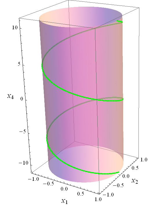
The purpose of the present work is to express this reduction explicitly in terms of the first fundamental form of the helicoidal surfaces under consideration and to determine the corresponding geodesics through quadrature formulas. We specify the assumptions under which these formulas reconstruct unit-speed geodesics and distinguish the non-constant-meridian solutions covered by the quadratures from geodesics with a constant meridian parameter, which require a separate characterization. As illustrative applications, we present two examples and use Mathematica 7 to plot the three-dimensional projection of the first helicoidal surface together with its corresponding projected geodesic. The second example examines a variable metric and verifies smooth continuation through a turning point.
In this section, we recall some fundamental definitions of curves and surfaces in \(4\)-dimensional Euclidean space \(\mathbb{R}^{4}\). Let \(x=(x_1,x_2,x_3,x_4)\) and \(y=(y_1,y_2,y_3,y_4)\) be arbitrary vectors in \(\mathbb{R}^4\). The standard Euclidean inner product on \(\mathbb{R}^4\) is defined by \[\langle x,y\rangle =\sum_{i=1}^{4}x_i y_i.\]
The corresponding Euclidean norm is induced by this inner product, and its value is given by \[\|x\|=\sqrt{\langle x,x\rangle} =\left(\sum_{i=1}^{4}x_i^2\right)^{1/2}.\]
A regular parametrized curve is an immersion \(\alpha :I \to \mathbb{R}^{4}\), where \(I\subseteq\mathbb{R}\) is an open real interval, that is, its derivative \(\dot\alpha=d\alpha/dt\) is nonzero at every point of the parameter interval. The arc-length parameter of \(\alpha\) in \(\mathbb{R}^{4}\) is \[s(t)=\int _{t_{0} }^{t}\left\|\dot\alpha(\xi)\right\|d\xi.\]
A regular curve \(\alpha\) is called a unit-speed curve if \(\|\dot\alpha(t)\|=1\) for every parameter value \(t\in I\subset\mathbb{R}\). Thus, its parameter measures signed arc length from a chosen initial point.
A parametrized surface element in \(\mathbb{R}^4\) is defined as an immersion \(\varphi:U\to\mathbb{R}^4\) of the form \(\varphi(u,v)=(\varphi_1(u,v),\ldots,\varphi_4(u,v))\), where \(U\subseteq\mathbb{R}^2\) is an open set (see [7]). The functions \(u\) and \(v\) are called the parameters of the parametrization. For fixed constants \(v_0\) and \(u_0\), respectively, the curves \(\alpha(u)=\varphi(u,v_0)\) and \(\beta(v)=\varphi(u_0,v)\) are called the \(u\)-parameter curve and the \(v\)-parameter curve, respectively.
The first fundamental form (line element) of a parametrized surface \(\varphi\) is given by \[ g:=ds^{2}=Edu^{2}+2Fdudv+Gdv^{2},\tag{1}\] where \(E=\langle \varphi_{u},\varphi_{u}\rangle\), \(F=\langle \varphi_{u},\varphi_{v}\rangle\), and \(G=\langle \varphi_{v},\varphi_{v}\rangle\) are the coefficients of the first fundamental form. Here, \(\varphi_{u}=\partial\varphi/\partial u\) and \(\varphi_{v}=\partial\varphi/\partial v\) are tangent vectors of the parameter curves of the surface element. In addition, the plane tangent to the surface element at the point \(p=\varphi(u,v)=\varphi(q)\) is identified with the vector space \(\operatorname{span}\{\varphi_{u}(q), \varphi_{v}(q)\}\).
The definitions and parametrizations of rotational and helicoidal surfaces in \(\mathbb{R}^4\) were given by Hieu and Thang [6], as follows.
Let \(\gamma:I\to H\) be a regular parametrized curve in a \(3\)-dimensional hyperplane \(H\subset\mathbb{R}^4\), and let \(P\) be a \(2\)-dimensional plane contained in \(H\). A rotational surface in \(\mathbb{R}^4\) is generated by rotating \(\gamma\) through a one-parameter family of rotations that fixes \(P\) pointwise. If the curve is simultaneously translated along a line \(l\) parallel to \(P\), with the translation distance proportional to the rotation parameter, the resulting surface is called a helicoidal surface in \(\mathbb{R}^4\).
Let \((x_{1},x_{2},x_{3},x_{4})\) denote the standard coordinates of \(\mathbb{R}^{4}\), and let \(\{e_{1},e_{2},e_{3},e_{4}\}\) be the corresponding standard orthonormal basis. We consider the \(3\)-dimensional hyperplane \[H=\operatorname{span}\{e_{1},e_{3},e_{4}\},\] the \(2\)-dimensional plane \[P=\operatorname{span}\{e_{3},e_{4}\},\] and the line \[l=\operatorname{span}\{e_{3}\}\subset P.\]
Let \(I\subset\mathbb{R}\) be an interval, and consider the profile curve \(\gamma:I\to H\) defined by \[\gamma(u)=\bigl(x_1(u),0,x_3(u),x_4(u)\bigr), \qquad u\in I,\] where \(x_1,x_3,x_4\in C^3(I)\) and \(x_1(u)>0\) for all \(u\in I\).
We consider a simple rotation in the \(2\)-dimensional plane \(\operatorname{span}\{e_1,e_2\}\), which fixes \(P=\operatorname{span}\{e_3,e_4\}\) pointwise, together with a translation along \(l=\operatorname{span}\{e_3\}\). Let \(v\in\mathbb{R}\) denote the rotation parameter and \(\lambda\in\mathbb{R}\) the pitch parameter. The resulting helicoidal surface is parametrized by \[ \varphi(u,v)= \bigl( x_1(u)\cos v,\, x_1(u)\sin v,\, x_3(u)+\lambda v,\, x_4(u) \bigr), \qquad (u,v)\in I\times\mathbb{R}.\tag{2}\]
Here, \(v\) represents the rotation angle, while \(\lambda v\) specifies the translational displacement along \(l\). Thus, the rotation acts in \(\operatorname{span}\{e_1,e_2\}\), whereas the translation occurs along \(l=\operatorname{span}\{e_3\}\). We assume that \(\varphi\) is regular, so that its first fundamental form is positive definite; equivalently, \(\Delta(u)=E(u)G(u)-F(u)^2>0.\)
If \(x_{3}\) is constant on \(I\), the resulting surface is called a right helicoidal surface. In the special case \(\lambda=0\), the translational component vanishes, while the rotational action remains unchanged. Consequently, (2) parametrizes a rotational surface in \(\mathbb{R}^{4}\). If \(x_{4}\) is constant on \(I\), the surface lies in a \(3\)-dimensional Euclidean affine subspace and reduces to a helicoidal surface in \(\mathbb{R}^{3}\); see [6,8].
In this section, we find the parametrizations of geodesics on helicoidal surfaces in \(4\)-dimensional Euclidean space.
We consider the helicoidal surface parametrized by Eq. (2). Its tangent vectors are \[\begin{aligned} \varphi_u &= \left( x_1’\cos v,\, x_1’\sin v,\, x_3′,\, x_4′ \right),\\ \varphi_v &= \left( -x_1\sin v,\, x_1\cos v,\, \lambda,\, 0 \right). \end{aligned}\]
Consequently, the coefficients of the first fundamental form are \[\begin{aligned} E&=(x_1′)^2+(x_3′)^2+(x_4′)^2,\\ F&=\lambda x_3′,\\ G&=x_1^2+\lambda^2. \end{aligned}\]
In particular, the parameter curves are orthogonal if and only if \(F=0\), that is, \(\lambda x_3’=0\). Thus, if \(\lambda\neq0\), orthogonality holds precisely when \(x_3’=0\).
The first fundamental form is therefore \[g= \big((x_1′)^2+(x_3′)^2+(x_4′)^2\big)\,du^2 +2\lambda x_3’\,du\,dv +\big(x_1^2+\lambda^2\big)\,dv^2;\] see, for example, [6,8]. Babaarslan studies loxodromes on this class of surfaces, so that reference supports the geometric parametrization and metric coefficients rather than the geodesic characterization established below.
A curve on the surface can be written as \[\alpha(t)=\varphi(u(t),v(t)) = \big( x_1(u(t))\cos v(t),\, x_1(u(t))\sin v(t),\, x_3(u(t))+\lambda v(t),\, x_4(u(t)) \big).\]
Throughout this section, primes denote derivatives with respect to \(u\), and dots denote derivatives with respect to the curve parameter \(t\). As we mentioned earlier, we assume that the surface is regular, so that \[\Delta(u)=E(u)G(u)-F(u)^2>0.\]
The energy Lagrangian associated with the first fundamental form is \[L= \frac12\left( E\dot u^{\,2} +2F\dot u\dot v +G\dot v^{\,2} \right).\]
The Euler–Lagrange equations are \[\frac{d}{dt}\frac{\partial L}{\partial\dot u} -\frac{\partial L}{\partial u}=0, \qquad \frac{d}{dt}\frac{\partial L}{\partial\dot v} -\frac{\partial L}{\partial v}=0.\]
Since the coefficients of the first fundamental form depend only on \(u\), a direct calculation yields the following system of geodesic equations: \[\begin{aligned} E\ddot u+F\ddot v +\frac{E’}{2}\dot u^2 -\frac{G’}{2}\dot v^2&=0,\notag\\ F\ddot u+G\ddot v +F’\dot u^2+G’\dot u\dot v&=0. \end{aligned}\tag{3}\]
Because \(v\) is a cyclic coordinate, the second Euler–Lagrange equation yields the conserved quantity \[F\dot u+G\dot v=J,\tag{4}\] where \(J\in\mathbb R\) is constant along each geodesic. Thus, \[\dot v=\frac{J-F\dot u}{G}.\tag{5}\]
We now consider unit-speed curves, for which \[\|\dot\alpha(t)\|^2=1.\]
Equivalently, \[E\dot u^{\,2}+2F\dot u\dot v+G\dot v^{\,2}=1.\tag{6}\]
Substituting (5) into this identity gives \[\left(E-\frac{F^2}{G}\right)\dot u^{\,2} +\frac{J^2}{G}=1.\]
Since \(\Delta=EG-F^2\), we obtain \[\dot u^{\,2}=\frac{G-J^2}{\Delta}.\tag{7}\]
We first consider geodesic segments on which \(G(u)>J^2\). On such a segment, \(\dot u\neq0\), and its sign is constant. Denoting this sign by \(\varepsilon\in\{-1,1\}\), we have \[\dot u=\varepsilon \sqrt{\frac{G-J^2}{\Delta}}, \qquad \frac{dt}{du} =\varepsilon\sqrt{\frac{\Delta}{G-J^2}}.\]
For initial values \(u(t_0)=u_0\) and \(v(t_0)=v_0\), integration yields \[t-t_0 = \varepsilon\int_{u_0}^{u(t)} \sqrt{\frac{\Delta(s)}{G(s)-J^2}}\,ds.\tag{8}\]
In general, this relation determines \(u(t)\) implicitly.
Furthermore, from (5), \[\frac{dv}{du} =\frac{\dot v}{\dot u} =\frac{J}{G\dot u}-\frac{F}{G}.\]
Using the expression for \(\dot u\), we obtain \[\frac{dv}{du} = \varepsilon\frac{J\sqrt{\Delta}} {G\sqrt{G-J^2}} -\frac{F}{G}.\]
Integrating from \(u_0\) to \(u(t)\) gives \[v(t)=v_0+ \int_{u_0}^{u(t)} \left( \varepsilon\frac{J\sqrt{\Delta(s)}} {G(s)\sqrt{G(s)-J^2}} -\frac{F(s)}{G(s)} \right)\,ds.\tag{9}\]
The same branch sign \(\varepsilon\) must be used in both (8) and (9).
We next verify that the curves reconstructed from these quadratures satisfy the full geodesic system. Let \[R_u= E\ddot u+F\ddot v +\frac{E’}{2}\dot u^2 -\frac{G’}{2}\dot v^2,\] and \[R_v= F\ddot u+G\ddot v +F’\dot u^2+G’\dot u\dot v,\] denote the left-hand sides of the two equations in (3), respectively. Direct differentiation of the Lagrangian gives \[\frac{dL}{dt}=\dot uR_u+\dot vR_v.\tag{10}\]
The reconstructed curves satisfy the conservation law (4), and hence \[R_v=\frac{d}{dt}(F\dot u+G\dot v)=0.\]
They also satisfy the unit-speed identity (6), so \(L=\tfrac12\) and \(dL/dt=0\). Therefore, (10) implies \[\dot uR_u=0.\]
Since \(\dot u\neq0\) on the branch under consideration, we conclude that \(R_u=0\). Thus both Euler–Lagrange equations are satisfied, proving that the reconstructed curves are unit-speed geodesics.
Conversely, every unit-speed geodesic segment on which \(G(u)>J^2\) and \(\dot u\) has a fixed, non-zero sign satisfies (4) and (6), and therefore admits the representation (8)–(9). Hence, these quadratures characterize precisely the geodesic segments in this domain.
Finally, the case \(\dot u=0\) must be treated separately because the preceding quadrature derivation does not apply. For a constant-\(u\) curve, let \[u(t)=u_*.\]
The geodesic system (3) reduces to \[F(u_*)\ddot v-\frac12G'(u_*)\dot v^2=0, \qquad G(u_*)\ddot v=0.\]
Since \(G(u_*)=x_1(u_*)^2+\lambda^2>0\), the second equation gives \(\ddot v=0\). The first then implies \(G'(u_*)=0\), provided the curve has non-zero speed. Conversely, if \(G'(u_*)=0\), the curve \[u(t)=u_*, \qquad v(t)=v_0\pm\frac{t-t_0}{\sqrt{G(u_*)}},\tag{11}\] satisfies both equations in (3) and has unit speed. Thus, a constant-\(u\) curve is a unit-speed geodesic if and only if \[G'(u_*)=0.\]
For the helicoidal surface considered here, \[G'(u)=2x_1(u)x_1′(u).\]
Since \(x_1(u_*)>0\), this criterion is equivalent to \(x_1′(u_*)=0.\) These constant-\(u\) geodesics are not covered by the quadrature formulas (8)–(9). Thus, we give the following theorem.
Theorem 1 (Local Quadrature Representation of Non-Constant-\(u\) Geodesics). Let \(\varphi:I\times\mathbb{R}\to\mathbb{R}^4\) be a \(C^3\) regular parametrization of the helicoidal surface given by (2), with the first fundamental form \[g=E(u)\,du^2+2F(u)\,du\,dv+G(u)\,dv^2,\] where \(\Delta(u)=E(u)G(u)-F(u)^2>0\) for all \(u\in I\). Let \(K\subseteq\mathbb{R}\) be an interval, and let \(\alpha:K\to\varphi(I\times\mathbb{R})\) be a \(C^3\), immersed, unit-speed geodesic on the helicoidal surface expressed in local coordinates as \(\alpha(t)=\varphi(u(t),v(t))\). Define the conserved Clairaut-type quantity \[J=F(u(t))\dot u(t)+G(u(t))\dot v(t).\]
Suppose that \(G(u(t))>J^2\) for all \(t\in K\), and that \(\dot u(t)\) has a fixed, non-zero sign on \(K\). Denote this sign by \(\varepsilon\in\{-1,1\}\). If \(u(t_0)=u_0\) and \(v(t_0)=v_0\) for some \(t_0\in K\), then the geodesic admits the local representation \[t-t_0 = \varepsilon\int_{u_0}^{u(t)} \sqrt{\frac{\Delta(s)}{G(s)-J^2}}\,ds,\tag{12}\] and \[v(t)=v_0+\int_{u_0}^{u(t)} \left( \varepsilon\frac{J\sqrt{\Delta(s)}} {G(s)\sqrt{G(s)-J^2}} -\frac{F(s)}{G(s)} \right)\,ds.\tag{13}\]
Conversely, let \(u_0\in I\), \(v_0\in\mathbb{R}\), \(J\in\mathbb{R}\), and \(\varepsilon\in\{-1,1\}\) satisfy \(G(u_0)>J^2\). Then, on a sufficiently small interval containing \(t_0\), formulas (12)–(13) locally determine a unit-speed geodesic with initial data \[u(t_0)=u_0,\quad v(t_0)=v_0,\quad \dot u(t_0)= \varepsilon\sqrt{\frac{G(u_0)-J^2}{\Delta(u_0)}}.\]
Eq. (12) determines \(u(t)\) implicitly in general; an explicit expression requires evaluating and inverting the integral. The representation is valid on intervals where \(G(u)>J^2\) and \(\dot u\) does not change sign. It does not include constant-\(u\) geodesics, which are characterized separately below.
Remark 1 (Intrinsic Reduction and Relation to Bour’s Theorem). Let \[g=E(u)\,du^2+2F(u)\,du\,dv+G(u)\,dv^2,\] be the induced metric on a coordinate neighborhood of the helicoidal surface, with \(G(u)>0\) and \(\Delta(u)=E(u)G(u)-F(u)^2>0\). Introduce the local coordinates \[w=v+\int_{u_0}^{u}\frac{F(s)}{G(s)}\,ds, \qquad r=\int_{u_0}^{u}\sqrt{\frac{\Delta(s)}{G(s)}}\,ds.\]
Since \(dr/du>0\), these define valid local coordinates, and the metric becomes \[g=dr^2+G(u(r))\,dw^2.\]
Consequently, the conserved momentum and the resulting quadrature representation in Theorem 1 are instances of the standard reduction for a metric admitting a Killing coordinate. The corresponding local integral construction and its converse are already present in the invariant-surface setting of Montaldo and Onnis [5]; the present formulas express that intrinsic reduction in the original helicoidal coordinates.
This observation is consistent with Bour’s theorem for helicoidal surfaces in \(\mathbb R^4\) established by Hieu and Thang [6]. In particular, if a local isometry maps the helicoidal surface to a rotational surface, it maps every geodesic of the former to a geodesic of the latter, preserving its arc-length parameter. Thus, the quadratures derived here also describe the corresponding geodesics on the isometric rotational surface, after applying the isometry.
The additional information provided here is an explicit formulation in the original parameters of the helicoidal surface, together with a verification of the full geodesic equations and a separate characterization of constant-\(u\) geodesics. Indeed, a unit-speed curve with \(u(t)\equiv u_*\) is a geodesic if and only if \(G'(u_*)=0\), in which case \[u(t)=u_*, \qquad v(t)=v_0\pm\frac{t-t_0}{\sqrt{G(u_*)}}.\]
For the helicoidal parametrization considered here, \(G(u)=x_1(u)^2+\lambda^2\). If \(x_1(u)>0\), the condition \(G'(u_*)=0\) is equivalent to \(x_1′(u_*)=0\). These constant-\(u\) geodesics are not covered by the quadrature formulas requiring \(\dot u\ne0\).
Lemma 1 (Characterization of Constant-\(u\) Geodesics). Let \(\varphi:I\times\mathbb R\to\mathbb R^4\) be a \(C^3\) regular parametrization of the helicoidal surface with the first fundamental form \[g=E(u)\,du^2+2F(u)\,du\,dv+G(u)\,dv^2, \qquad \Delta(u)=E(u)G(u)-F(u)^2>0.\]
Assume that \(G(u)>0\) on \(I\). For any \(u_*\in I\) and \(v_0\in\mathbb R\), consider the curve \[u(t)=u_*, \qquad v(t)=v_0\pm\frac{t-t_0}{\sqrt{G(u_*)}}.\tag{14}\]
Then the curve defined by (14) is a unit-speed geodesic if and only if \[G'(u_*)=0.\]
Proof. Since the metric coefficients depend only on \(u\), the geodesic equations associated with the metric \(g\) are \[\ddot u+ \Gamma^u_{uu}\dot u^2+ 2\Gamma^u_{uv}\dot u\dot v+ \Gamma^u_{vv}\dot v^2=0,\] and \[\ddot v+ \Gamma^v_{uu}\dot u^2+ 2\Gamma^v_{uv}\dot u\dot v+ \Gamma^v_{vv}\dot v^2=0.\]
The relevant Christoffel symbols, obtained from the inverse metric and its derivatives, are \(\Gamma^u_{vv}=-\frac{GG’}{2\Delta}\) and \(\Gamma^v_{vv}=\frac{FG’}{2\Delta}\), where \(\Delta=EG-F^2>0\). Consider a constant-\(u\) curve \(\alpha(t)=\varphi(u_*,v(t))\).
Since \(\dot u=\ddot u=0\), the first geodesic equation reduces to \[-\frac{G(u_*)G'(u_*)}{2\Delta(u_*)}\dot v^{\,2}=0.\]
Because the curve is immersed, \(\dot v\neq0\). Together with \(G(u_*)>0\) and \(\Delta(u_*)>0\), this implies \(G'(u_*)=0\). Hence, this condition is necessary for the curve to be a geodesic.
Conversely, suppose that \(G'(u_*)=0\). For the affine function \(v(t)\) in (14), we also have \(\ddot v=0\). Substituting \(\dot u=\ddot u=\ddot v=0\) and \(G'(u_*)=0\) into both geodesic equations shows that they are satisfied. Therefore, the constant-\(u\) curve is a geodesic. Its squared speed is \(\|\dot\alpha(t)\|^2=G(u_*)\dot v^{\,2}\). Consequently, choosing \(\dot v=\pm1/\sqrt{G(u_*)}\) yields a unit-speed parametrization. We conclude that a constant-\(u\) curve admits a unit-speed geodesic parametrization if and only if \(G'(u_*)=0\). ◻ \(\square\)
Remark 2 (Turning Points and Geodesic Orbits). The condition \(G(u)=J^2\) marks the boundary of the monotone representation given by equations (12) and (13). However, this condition alone does not determine whether a geodesic has a turning point or follows a geodesic orbit. To distinguish these possibilities, let \(t_*\) be a finite parameter value at which \(\dot u(t_*)=0\), and set \(u_*=u(t_*)\).
At \(t=t_*\), the unit-speed condition gives \[G(u_*)\dot v(t_*)^2=1.\]
The full geodesic equations reduce to \[E(u_*)\ddot u(t_*)+F(u_*)\ddot v(t_*) -\frac12G'(u_*)\dot v(t_*)^2=0,\] \[F(u_*)\ddot u(t_*)+G(u_*)\ddot v(t_*)=0.\]
Eliminating \(\ddot v(t_*)\) and using \(\dot v(t_*)^2=1/G(u_*)\), we obtain \[{\ddot u(t_*)=\frac{G'(u_*)}{2\Delta(u_*)}}, \text{ and } \Delta=EG-F^2.\]
If \(G'(u_*)\neq0\), then \(\ddot u(t_*)\neq0\), so \(u_*\) is an ordinary local turning point of the profile coordinate. The geodesic continues smoothly through \(t_*\), with \(\dot u\) changing sign. Thus, the continuation is described by the opposite square-root branch of the first-order equation on the other side of the turning point.
If \(G'(u_*)=0\), then \(\ddot u(t_*)=0\). In this case, the initial data \[u(t_*)=u_*, \qquad \dot u(t_*)=0, \qquad \dot v(t_*)=\pm\frac{1}{\sqrt{G(u_*)}},\] generate a constant-\(u\) geodesic, provided \(G(u_*)>0\). Indeed, the curve \[u(t)=u_*, \qquad v(t)=v(t_*)\pm\frac{t-t_*}{\sqrt{G(u_*)}},\] satisfies the full geodesic equations precisely when \(G'(u_*)=0\). By uniqueness of solutions to the smooth second-order geodesic system, any geodesic with these initial data coincides locally with this orbit.
Consequently, a zero of \(G-J^2\) may correspond either to an ordinary turning point or to a geodesic orbit. The continuation through such a point must be determined by the full second-order geodesic system, rather than by assigning an arbitrary sign to the square-root in the first-order equation.
In this section, we present two examples of geodesics on helicoidal surfaces. The first provides an explicit solution and a projection visualized using Mathematica 7; the second verifies the quadrature formulas for a variable metric and examines the behavior at a turning point.
Example 1. Consider the profile functions \[x_1(u)=1,\qquad x_3(u)=\frac{u}{2},\qquad x_4(u)=\frac{\sqrt{3}}{2}u, \qquad \lambda=1.\]
Then, the helicoidal surface is parametrized by \[ \varphi(u,v) = \left( \cos v,\, \sin v,\, \frac{u}{2}+v,\, \frac{\sqrt{3}}{2}u \right).\tag{15}\]
Since \[(x_1′)^2+(x_3′)^2+(x_4′)^2=1,\] the profile curve is unit-speed. Moreover, the coefficients of the first fundamental form are \[E=1,\qquad F=\frac12,\qquad G=2,\] and hence \[\Delta=EG-F^2=\frac74.\]
This example serves as a consistency check for the general geodesic formulas. Since the coefficients of the first fundamental form are constant, all Christoffel symbols vanish in the coordinates \((u,v)\). Consequently, the geodesic equations reduce to \[\ddot u=0,\qquad \ddot v=0,\] so the geodesics have affine coordinate functions in these surface coordinates. Accordingly, this example does not illustrate the non-trivial behavior associated with a variable metric coefficient or a turning point. We retain it to provide an explicit geodesic and to illustrate the geometry of its orthogonal projection.
Let \[J=-\frac12,\qquad u(0)=0,\qquad v(0)=0.\]
From the reduced unit-speed equation \(\dot{u}^{\,2}=\frac{G-J^2}{\Delta},\) we obtain \[\dot{u}^{\,2} =\frac{2-\frac14}{\frac74}=1.\]
Choosing the positive branch gives \[\dot u=1,\qquad u(t)=t.\]
On the other hand, the conserved-momentum equation \[F\dot u+G\dot v=J,\] becomes \[\frac12\dot u+2\dot v=-\frac12.\]
Since \(\dot u=1\), we obtain \[\dot v=-\frac12.\]
Using \(v(0)=0\), it follows that \[v(t)=-\frac{t}{2}.\]
Consequently, the corresponding geodesic on the helicoidal surface is \[ \alpha(t) = \left( \cos\frac{t}{2},\, -\sin\frac{t}{2},\, 0,\, \frac{\sqrt{3}}{2}t \right).\tag{16}\]
Its speed is constant and equal to one, since \[\|\alpha'(t)\|^2 =\frac14+\frac34=1.\]
Therefore, the arc length of the geodesic segment between \(-4\pi\) and \(4\pi\) is \[l(\alpha) =\int_{-4\pi}^{4\pi}\|\alpha'(t)\|\,dt =8\pi.\]
For visualization, consider the orthogonal projection onto the \((x_1,x_2,x_4)\) coordinate space. The projected helicoidal surface is \[\phi(u,v) = \left( \cos v,\, \sin v,\, \frac{\sqrt{3}}{2}u \right),\] which is a circular cylinder. The corresponding projected geodesic is \[\sigma(t) = \left( \cos\frac{t}{2},\, -\sin\frac{t}{2},\, \frac{\sqrt{3}}{2}t \right),\] which is a helix lying on this cylinder. Since the omitted coordinate satisfies \(x_3(t)\equiv0\) along the geodesic, the projection preserves its length. Hence, \[l(\sigma) =\int_{-4\pi}^{4\pi}\|\sigma'(t)\|\,dt =8\pi=l(\alpha).\]
The \(3\)-dimensional visualization of the projected surface and its geodesic is presented in Figure 1.
Example 2. Consider the profile functions \[x_1(u)=u,\qquad x_3(u)=0,\qquad x_4(u)=u, \qquad \lambda=1,\] defined for \(u>0\). The corresponding helicoidal surface is parametrized by \[ \varphi(u,v) = \left( u\cos v,\, u\sin v,\, v,\, u \right), \qquad u>0,\quad v\in\mathbb R.\tag{17}\]
Its tangent vectors are \[\varphi_u=(\cos v,\sin v,0,1), \qquad \varphi_v=(-u\sin v,u\cos v,1,0).\]
These vectors are linearly independent, so \(\varphi\) is an immersion.
The coefficients of the first fundamental form are \[E=2,\qquad F=0,\qquad G=u^2+1,\] and \[\Delta=EG-F^2=2(u^2+1)>0.\]
In contrast to Example 1, the coefficient \(G\) is non-constant.
Let \(J=2\). The conserved-momentum equation \(F\dot u+G\dot v=J\) and the unit-speed relation yield \[ \dot v=\frac{2}{u^2+1}, \qquad \dot u^{\,2}=\frac{u^2-3}{2(u^2+1)}.\tag{18}\]
Thus, the quadrature formulas become \[ t-t_0 = \varepsilon\int_{2}^{u(t)} \sqrt{\frac{2(s^2+1)}{s^2-3}}\,ds,\tag{19}\] and \[ v(t) = v_0+ \varepsilon\int_{2}^{u(t)} \frac{2\sqrt{2}} {\sqrt{s^2+1}\sqrt{s^2-3}}\,ds,\tag{20}\] where \(\varepsilon=\operatorname{sgn}(\dot u)\). In (20), the factor \(\sqrt{s^2+1}\) in the denominator follows by simplifying \(J\sqrt{\Delta}/G\) before division by \(\sqrt{G-J^2}\). These formulas apply on a monotone interval on which \(u>\sqrt{3}\).
Choose the initial conditions \[u(t_0)=2,\qquad v(t_0)=0,\qquad \dot u(t_0)=-\frac{1}{\sqrt{10}}, \qquad \dot v(t_0)=\frac25.\]
They satisfy the unit-speed condition: \[E(2)\dot u(t_0)^2+G(2)\dot v(t_0)^2 = 2\left(\frac1{10}\right) +5\left(\frac4{25}\right)=1.\]
Moreover, \(F(2)\dot u(t_0)+G(2)\dot v(t_0)=2,\) so the conserved momentum is indeed \(J=2\). The corresponding branch is \(\varepsilon=-1\).
The boundary of the monotone representation occurs at \(u_*=\sqrt{3},\quad G(u_*)=J^2=4.\) Since \(G'(u_*)=2\sqrt{3}\ne0,\) this point is an ordinary turning point rather than a constant-\(u\) geodesic. To examine the continuation, we use the full geodesic system: \[ 2\ddot u-u\dot v^2=0,\tag{21}\] \[ (u^2+1)\ddot v+2u\dot u\dot v=0.\tag{22}\]
At the turning point, \(\dot u(t_*)=0\). The unit-speed condition gives \[\dot v(t_*)=\frac{1}{\sqrt{u_*^2+1}}=\frac12,\] for the chosen positive value of the conserved momentum. Therefore, equation (21) yields \[\ddot u(t_*) =\frac{u_*}{2}\dot v(t_*)^2 =\frac{\sqrt{3}}{8}>0.\]
Hence, \(\dot u\) changes from negative to positive as the geodesic passes through \(t_*\). The geodesic continues smoothly, but the quadrature representation must be applied separately on the two monotone portions, with opposite signs of \(\dot u\).
We next verify that the reconstructed curve satisfies both geodesic equations. Differentiating (18) on either monotone interval gives \[\ddot u=\frac{2u}{(u^2+1)^2}, \qquad \ddot v=-\frac{4u\dot u}{(u^2+1)^2}.\]
Substitution into (21) yields \[2\ddot u-u\dot v^2 = \frac{4u}{(u^2+1)^2} -\frac{4u}{(u^2+1)^2}=0.\]
Similarly, substitution into (22) gives \[\begin{aligned} (u^2+1)\ddot v+2u\dot u\dot v &=-\frac{4u\dot u}{u^2+1} +\frac{4u\dot u}{u^2+1}\\ &=0. \end{aligned}\]
Thus, the reconstructed curve satisfies both Euler–Lagrange equations on each monotone interval.
At the turning point, the geodesic extends smoothly as the solution of the full second-order system with initial data \[u(t_*)=\sqrt{3},\qquad \dot u(t_*)=0,\qquad \dot v(t_*)=\frac12.\]
Because the metric coefficients are smooth and \(\Delta>0\), local uniqueness of the geodesic initial-value problem determines this continuation.
This example demonstrates that the quadrature formulas apply to a helicoidal surface with a non-constant induced metric and that the boundary \(G=J^2\) can correspond to an ordinary turning point rather than a constant-\(u\) geodesic. It also illustrates why continuation through a turning point must be governed by the full second-order geodesic system rather than by an arbitrary choice of square-root sign.
In this paper, we derived a first-order characterization and a local quadrature representation for geodesics on a class of helicoidal surfaces in \(4\)-dimensional Euclidean space. The presence of the cyclic coordinate yields the conserved quantity associated with the helicoidal symmetry. Combining this conserved quantity with the unit-speed condition reduces the geodesic equations to a first-order system and, on an interval where the profile parameter is monotone, to the corresponding local quadrature formula.
The resulting representation is subject to the admissibility condition \(G-J^{2}>0,\) and therefore describes geodesic segments on admissible monotone branches. At points where \(G=J^{2}\), the chosen graph representation may cease to be valid because the corresponding profile parameter can have a turning point. Thus, the obtained quadrature should be understood as a local representation rather than a parametrization of every complete geodesic.
The first example provides an explicit verification of the derived equations. For the selected helicoidal surface, the geodesic equations can be solved analytically, yielding \[\alpha(t)= \left( \cos\frac{t}{2}, -\sin\frac{t}{2}, 0, \frac{\sqrt{3}}{2}t \right),\] and the length of the segment considered is \(l(\alpha)=8\pi.\) The corresponding projection used for visualization preserves the length in this particular example because the omitted coordinate is constant.
The second example complements this explicit solution by exhibiting a variable metric and an ordinary turning point at \(u=\sqrt{3}\). Its continuation satisfies the full second-order system, while the quadrature formulas require separate signs on the incoming and outgoing monotone branches. Together, the examples distinguish an explicitly integrable case from the local continuation problem.
The results establish a local geodesic description for the considered class of helicoidal surfaces in the Euclidean setting. Further analysis of special subclasses, such as developable, minimal, or Weingarten helicoidal surfaces, may provide additional geometric consequences of the derived characterization.
Acknowledgments: The authors express their sincere gratitude to the referee for the exceptionally thorough and insightful review. The referee’s constructive comments and valuable suggestions have significantly enhanced the overall quality, clarity, and rigor of the manuscript.
Author Contributions: All authors have read and approved the final version of the manuscript.
Conflicts of Interest: The authors declare that they have no competing interests.
Data Availability: No datasets were generated or analyzed in this theoretical study.
Funding Information: This research received no external funding.