
Burgers fluids represent a direct generalization of Oldroyd-B fluids introduced by Oldroyd [1]. Unlike the Maxwell and Oldroyd-B models they imply the upper-convected derivative of second order with respect to time of the first Rivlin-Ericksen tensor. The linearized form of the constitutive equations for these fluids was proposed by Burgers in 1935 [2]. Its extension to a frame-indifferent 3D form was developed by Krishnan and Rajagopal [3, 4]. The linear form of this model has been used to describe the behavior of different viscoelastic materials like asphalt, soil or cheese [3, 5]. A good accordance between the predictions of this model and the behavior of different specimens of sand-asphalt has been remarked by Lee and Markwick [6]. Saal and Labont [7] also proved that the mechanical response of asphalt can be well enough described by Burgers model. This model was also used to describe the transient creep properties of the earth’s mantle [8, 9] and, in the last time, many papers have studied steady or unsteady motions of incompressible Burgers fluids in different circumstances.
First exact solutions for the steady flow of incompressible Burgers fluids seem to be those of Ravindran et al. [10] in an orthogonal rheometer. It is a flow between two parallel plates which rotate with the same constant angular speed around two different axes. Steady or steady state solutions corresponding to Stokes’ problems for same fluids have been obtained by Hayat et al. [11] and Fetecau et al. [12]. Start-up solutions for same problems were established by Akram et al. [13] and Fetecau et al [14]. Interesting results regarding unsteady motions of incompressible Burgers fluids in cylindrical domains can be found in the papers of Tong and Shan [15], Tong and Hu [16], Fetecau et al. [17, 18], Khan et al. [19] and Raza et al. [20]. A magnetic field acting on an electrical conducting fluid in motion produces effects that can be utilized in different domains of physics and chemistry like MHD generators, plasma studies, astrological exploration, aerodynamics, geothermal energy excitations and hydrology.
Among more recent results regarding MHD motions of incompressible Burgers fluids in rectangular domains we mention those of Khan et al. [21], Abro et al. [22], Alqahtani and Khan [23], Hussain et al. [24] and Fetecau et al. [25]. It is worth to mention the fact that in the last reference [25], unlike in the previous ones, the oscillatory shear stresses have been prescribed on the boundary. Unfortunately, exact solutions for MHD motions of incompressible Burgers fluids in cylindrical domains are few in the existing literature. The steady velocity fields corresponding to MHD flows of incompressible Burgers fluids due to increasing, decreasing or pulsating pressure gradients in an infinite circular cylinder have been obtained by Rabia et al. [26]. Permanent velocity fields for MHD motions of same fluids induced by constant or oscillatory pressure gradients between two infinite coaxial circular cylinders were recently provided by Fetecau [27]. Semi-analytical expressions for velocity and skin friction have been also recently obtained by Isa and Musa [28] for MHD Couette flow of incompressible Burgers fluids between two coaxial circular cylinders.
Our interest here is to find exact solutions for the axial Couette flow of incompressible Burgers fluids in an infinite circular cylinder that slides with an arbitrary time-dependent velocity along its symmetry axis. The influence of magnetic field is taken into consideration. General analytic expressions are established for the dimensionless velocity field and non-trivial shear stress. They can generate exact solutions for any motion of the respective fluids of this kind and the problem in discussion is completely solved. For validation, the fluid velocity is presented in two different forms and their equivalence is graphically proved for a given motion. The influence of magnetic field on the fluid motion is graphically presented and discussed. It is proved that the fluid moves slower in the presence of a magnetic field except a small vicinity of the symmetry axis of cylinder at small values of the time t.
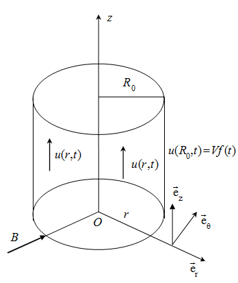
Let us assume that an electrically conducting upper-convected incompressible Burgers fluid (ECUCIBF) is at rest in an infinite circular cylinder. At the moment \(t=0^{+}\) the cylinder starts to slide along its symmetry axis with the velocity \(Vf(t)\) and a circular magnetic field of constant strength B acts perpendicular to the cylinder axis [26, 29]. The piecewise function \(f(\cdot )\) has zero value in \(t=0\) and V is constant velocity. Owing to the shear the fluid begins to move and the velocity vector u corresponding to its movement is given by the relation [30] \[\label{GrindEQ__1_} \boldsymbol{\mathit{u}}=\boldsymbol{\mathit{u}}(r,t)=u(r,t)\boldsymbol{\mathrm{e}}_{z} , \tag{1}\] in a cylindrical coordinate system r, \(\theta\) and z in which \(\boldsymbol{\mathrm{e}}_{z}\) is the unit vector along the z-axis (Figure 1).
The constitutive equations of incompressible Burgers fluids are given by the relations [26] \[\label{GrindEQ__2_} \boldsymbol{\mathit{T}}=-p\boldsymbol{\mathit{I}}+\boldsymbol{\mathit{S}},\quad \left(1+a_{1} \frac{\delta }{\delta \mathit{t}} +a_{2} \frac{\delta ^{2} }{\delta \mathit{t}^{\mathit{2}} } \right)\mathit{S}=2\mu \left(1+a_{3} \frac{\delta }{\delta \mathit{t}} \right)\mathit{D}, \tag{2}\] where T is the stress tensor, S is the extra-stress tensor, D is the symmetric part of the velocity gradient, I is the identity tensor, p is the hydrostatic pressure, \(\mu\) is the fluid viscosity and \(a_{1} ,\, a_{2} ,\, a_{3}\) are material constants. If \(a_{2} =0\) one finds the constitutive equations of Oldroyd-B fluids and the constants \(a_{1} ,\, a_{3}\) are called relaxation and retardation times, respectively, while \(\delta /\delta t\) denotes the upper-convected time derivative. If we suppose that the extra-stress tensor S, like the velocity vector u, is also a function of r and t only, one can prove that the non-trivial shear stress \(\tau (r,t)=S_{rz} (r,t)\) satisfies the partial differential equation \[\label{GrindEQ__3_} \left(1+a_{1} \frac{\partial }{\partial \mathit{t}} +a_{2} \frac{\partial ^{2} }{\partial \mathit{t}^{\mathit{2}} } \right)\tau (r,t)=\mu \left(1+a_{3} \frac{\partial }{\partial \mathit{t}} \right)\frac{\partial u(r,t)}{\partial r} ;\, \, \, 0<r<R_{0} ,\, \, t>0, \tag{3}\] where \(R_{0}\) is the cylinder radius.
Supposing that the fluid is finitely conducting, its magnetic permeability is constant, the induced magnetic field is small enough and can be neglected, there is no surplus electric charge distribution inside and there is no pressure gradient in the z-direction, the balance of linear momentum reduces to the following partial differential equation [26] \[\label{GrindEQ__4_} \rho \frac{\partial u(r,t)}{\partial t} =\frac{\partial \tau (r,t)}{\partial r} +\frac{1}{r} \tau (r,t)-\sigma B^{2} u(r,t);\, \, \, 0<r<R_{0} ,\, \, t>0. \tag{4}\]
In above relation \(\rho\) is the fluid density and \(\sigma\) is the electrical conductivity. The two unknown functions \(u(r,t)\) and \(\tau (r,t)\) have to satisfy the next initial and boundary conditions \[\label{GrindEQ__5_} u(r,0)=0,\, \, \tau (r,0)=0,\, \, \left. \frac{\partial \tau (r,t)}{\partial t} \right|_{t=0} =0;\, \, \, 0<r<R_{0} , \tag{5}\] \[\label{GrindEQ__6_} u(R_{0} ,t)=Vf(t);\, \, \, t\ge 0. \tag{6}\]
By introducing the next non-dimensional variables and functions \[\label{GrindEQ__7_} \bar{r}=\frac{1}{R_{0} } r,\, \, \, \bar{t}=\frac{\nu }{R_{0}^{2} } t,\, \, \, \bar{u}=\frac{1}{V} u,\, \, \, \bar{\tau }=\frac{R_{0} }{\mu V} \tau ,\, \, \, \bar{f}(\bar{t})=f\left(\frac{R_{0}^{2} }{\nu } \bar{t}\right), \tag{7}\] where \(\nu =\mu /\rho\) is the kinematic viscosity of the fluid and dropping out the bar notation, one finds the following dimensionless forms \[\label{GrindEQ__8_} \left(1+\alpha \frac{\partial }{\partial \mathit{t}} +\beta \frac{\partial ^{2} }{\partial \mathit{t}^{\mathit{2}} } \right)\tau (r,t)=\left(1+\gamma \frac{\partial }{\partial \mathit{t}} \right)\frac{\partial u(r,t)}{\partial r} ;\, \, \, 0<r<1,\, \, t>0, \tag{8}\] \[\label{GrindEQ__9_} \frac{\partial u(r,t)}{\partial t} =\frac{\partial \tau (r,t)}{\partial r} +\frac{1}{r} \tau (r,t)-Mu(r,t);\, \, \, 0<r<1,\, \, t>0, \tag{9}\] of the governing Eqs. (3) and (4).
In above equations the constants \(\alpha ,\, \beta ,\, \gamma\) and the magnetic parameter M are defined by the next relations: \[\label{GrindEQ__10_} \alpha =\frac{\nu }{R_{0}^{2} } a_{1} ,\, \, \beta =\frac{\nu ^{2} }{R_{0}^{4} } a_{2} ,\, \, \gamma =\frac{\nu }{R_{0}^{2} } a_{3} ,\, \, M=\frac{\sigma B^{2} }{\mu } R_{0}^{2} . \tag{10}\]
In the existing literature the parameter \(\alpha\) is also called dimensionless relaxation time or “Weissenberg number”. The initial and boundary conditions (5) and (6) become \[\label{GrindEQ__11_} u(r,0)=0,\, \, \tau (r,0)=\left. \frac{\partial \tau (r,t)}{\partial t} \right|_{t=0} =0;\, \, \, 0<r<1, \tag{11}\] \[\label{GrindEQ__12_} u(1,t)=f(t);\, \, \, t\ge 0. \tag{12}\]
In the next, the system of partial differential Eqs. (8) and (9) with the initial and boundary conditions (11) and (12) will be solved by means of Laplace and finite Hankel transforms.
By applying the Laplace transform to the equalities (8) and (9) and bearing in mind the initial conditions (11) one finds that the Laplace transforms \(\hat{u}(r,s),\, \hat{\tau }(r,s)\) of \(u(r,t),\, \tau (r,t)\), respectively, satisfy the relations \[\label{GrindEQ__13_} \hat{\tau }(r,s)=\frac{\gamma {\kern 1pt} s+1}{\beta {\kern 1pt} s^{2} +\alpha {\kern 1pt} s+1} \frac{\partial \hat{u}(r,s)}{\partial r} , \tag{13}\] \[\label{GrindEQ__14_} s\hat{u}(r,s)=\frac{\partial \hat{\tau }(r,s)}{\partial r} +\frac{1}{r} \hat{\tau }(r,s)-M\hat{u}(r,s). \tag{14}\]
By substituting \(\hat{\tau }(r,s)\) from Eq. (13) in (14) one finds that \(\hat{u}(r,s)\) has to satisfy the next differential equation \[\label{GrindEQ__15_} \frac{\partial ^{2} \hat{u}(r,s)}{\partial r^{2} } +\frac{1}{r} \frac{\partial \hat{u}(r,s)}{\partial r} =a(s)\hat{u}(r,s);\, \, \, 0<r<1, \tag{15}\] with the boundary condition \[\label{GrindEQ__16_} \hat{u}(1,s)=\hat{f}(s). \tag{16}\]
The function \(a(\cdot )\) from Eq. (15) is given by the relation \[\label{GrindEQ__17_} a(s)=\frac{\beta {\kern 1pt} s^{3} +(\alpha +\beta M)s^{2} +(\alpha M+1)s+M}{\gamma {\kern 1pt} s+1} . \tag{17}\]
Now, by applying the finite Hankel transform (see Equations (A1) from Appendix A) to Eq. (15) and using the identity (A2) one finds that the finite Hankel transform \(\hat{u}_{H} (r_{n} ,s)\) of \(\hat{u}(r,s)\) is given by the relation \[\label{GrindEQ__18_} \hat{u}_{H} (r_{n} ,s)=\frac{\hat{f}(s)}{r_{n}^{2} +a(s)} r_{n} J_{1} (r_{n} ), \tag{18}\] or equivalently \[\label{GrindEQ__19_} \hat{u}_{H} (r_{n} ,s)=\frac{1}{r_{n} } J_{1} (r_{n} )\hat{f}(s)-\frac{1}{r_{n} } J_{1} (r_{n} )\hat{f}(s)\frac{a(s)}{r_{n}^{2} +a(s)} . \tag{19}\]
By applying the inverse finite Hankel transform to Eq. (19) and bearing in mind the entry 1 of Table X from Appendix C of the reference [31] one finds that \[\label{GrindEQ__20_} \hat{u}(r,s)=\hat{f}(s)-2\hat{f}(s)\sum _{n=1}^{\infty }\frac{a(s)}{r_{n}^{2} +a(s)} \frac{J_{0} (rr_{n} )}{r_{n} J_{1} (r_{n} )} . \tag{20}\]
In above relations \(J_{0} (\cdot )\) and \(J_{1} (\cdot )\) are standard Bessel functions of the first kind of zero and one order, respectively.
In order to apply the inverse Laplace transform to Eq. (20), we firstly write the ratio \(a(s)/[r_{n}^{2} +a(s)]\) in equivalent forms, namely \[\begin{aligned} \label{GrindEQ__21_} \frac{a(s)}{r_{n}^{2} +a(s)} =&1-r_{n}^{2} \frac{\gamma (s+1/\gamma )}{\beta (s+b_{0} /3)\{ [(s+b_{0} /3)^{2} -p_{n} ]+q_{n} (s+b_{0} /3)^{-1} \} }\notag\\ =&1-r_{n}^{2} \frac{\gamma }{\beta } \sum _{k=0}^{\infty }\frac{(-q_{n} )^{k} (s+b_{0} /3)^{-k} }{[(s+b_{0} /3)^{2} -p_{n} ]^{k+1} } -r_{n}^{2} \frac{3-\gamma {\kern 1pt} b_{0} }{3\beta } \sum _{k=0}^{\infty }\frac{(-q_{n} )^{k} (s+b_{0} /3)^{-k-1} }{[(s+b_{0} /3)^{2} -p_{n} ]^{k+1} } . \end{aligned} \tag{21}\]
In above relations the constants \(p_{n} ,\, q_{n} ,\, b_{0} ,\, b_{1n}\) and \(b_{2n}\) have the expressions \[\label{GrindEQ__22_} b_{0} =\frac{\alpha +\beta M}{\beta } ,\, \, p_{n} =\frac{b_{0}^{2} }{3} -b_{1n} ,\, \, q_{n} =b_{2n} -\frac{b_{0} b_{1n} }{3} +\frac{2b_{0}^{3} }{27} , \tag{22}\] \[\label{GrindEQ__23_} b_{1n} =\frac{1+\alpha M+\gamma {\kern 1pt} r_{n}^{2} }{\beta } ,\, \, b_{2n} =\frac{r_{n}^{2} +M}{\beta } . \tag{23}\]
Finally, applying the inverse Laplace transform to Eq. (20) and bearing in mind the relations (21) and (A3) from Appendix A one finds for the dimensionless velocity field \(u(r,t)\) the expression \[\begin{aligned} \label{GrindEQ__24_} u(r,t)=&f(t)-2f(t)*\sum _{n=1}^{\infty }\left\{\delta (t)-r_{n}^{2} \frac{\gamma }{\beta } \right. (-q_{n} )^{k} { e}^{-b_{0} t/3} G_{2,-k,k+1} (t,p_{n} )\notag\\ &-\left. r_{n}^{2} \frac{3-\gamma {\kern 1pt} b_{0} }{3\beta } (-q_{n} )^{k} { e}^{-b_{0} t/3} G_{2,-k-1,k+1} (t,p_{n} )\right\}\frac{J_{0} (rr_{n} )}{r_{n} J_{1} (r_{n} )} , \end{aligned} \tag{24}\] where \(\delta (\cdot )\) is the Dirac delta function, \(*\) denotes the convolution product and \[\label{GrindEQ__25_} G_{a,b,c} (t,d)=\sum _{j=0}^{\infty }\frac{d^{j} \Gamma (j+c)t^{(j+c)a-b-1} }{\Gamma (c)\Gamma (j+1)\Gamma ((j+c)a-b)} ;\, \, \, Re(ac-b)>0, \tag{25}\] is the Lorenzo-Hartley G-function [32].
By replacing \(\hat{u}(r,s)\) from Eq. (20) in the relation (13) one finds that \[\label{GrindEQ__26_} \hat{\tau }(r,s)=2\hat{f}(s)\frac{\gamma {\kern 1pt} s+1}{\beta {\kern 1pt} s^{2} +\alpha {\kern 1pt} s+1} \sum _{n=1}^{\infty }\frac{a(s)}{r_{n}^{2} +a(s)} \frac{J_{1} (rr_{n} )}{J_{1} (r_{n} )} . \tag{26}\]
Now, by applying the inverse Laplace transform to the relation \[\begin{aligned} \label{GrindEQ__27_} \frac{\gamma {\kern 1pt} s+1}{\beta {\kern 1pt} s^{2} +\alpha {\kern 1pt} s+1} =&\frac{\gamma }{\beta } \, \, \frac{s+\alpha /(2\beta )}{[s+\alpha /(2\beta )]^{2} -[\sqrt{\alpha ^{2} -4\beta } /(2\beta )]^{2} } \notag\\ &+\frac{2\beta -\alpha \gamma }{\beta \sqrt{\alpha ^{2} -4\beta } } \, \frac{\sqrt{\alpha ^{2} -4\beta } /(2\beta )}{[s+\alpha /(2\beta )]^{2} -[\sqrt{\alpha ^{2} -4\beta } /(2\beta )]^{2} } , \end{aligned} \tag{27}\] and bearing in mind the identities (A4) from Appendix A it results that \[\begin{aligned} \label{GrindEQ__28_} g(t)=&L^{-1} \left\{\frac{\gamma {\kern 1pt} s+1}{\beta {\kern 1pt} s^{2} +\alpha {\kern 1pt} s+1} \right\}=\frac{\gamma }{\beta } \, \left\{\cosh \left(\frac{\sqrt{\alpha ^{2} -4\beta } }{2\beta } t\right)\right. \notag\\ & +\left. \frac{2\beta -\alpha \gamma }{\gamma \sqrt{\alpha ^{2} -4\beta } } \sinh \left(\frac{\sqrt{\alpha ^{2} -4\beta } }{2\beta } t\right)\right\}\exp \left(-\frac{\alpha }{2\beta } t\right). \end{aligned} \tag{28}\]
Consequently, by applying the inverse Laplace transform to Eq. (26) and using the identities (21) and (28) one finds the dimensionless shear stress \(\tau (r,t)\) in the following form \[\begin{aligned} \label{GrindEQ__29_} \tau (r,t)=&2f(t)*g(t)\sum _{n=1}^{\infty }\frac{J_{1} (rr_{n} )}{J_{1} (r_{n} )} -\frac{2}{\beta } f(t)*g(t)*\sum _{n=1}^{\infty }r_{n}^{2} (-q_{n} )^{k} \exp \left(-\frac{b_{0} }{3} t\right) \notag\\ &\times \left\{\gamma {\kern 1pt} G_{2,-k,k+1} (t,p_{n} )-\frac{3-\gamma b_{0} }{3} G_{2,-k-1,k+1} (t,p_{n} )\right\}\frac{J_{1} (rr_{n} )}{J_{1} (r_{n} )} . \end{aligned} \tag{29}\]
Eq. (15) can be written as a Bessel equation, namely \[\label{GrindEQ__30_} r^{2} \frac{\partial ^{2} \hat{u}(r,s)}{\partial r^{2} } +r\frac{\partial \hat{u}(r,s)}{\partial r} +[ir\sqrt{a(s)} ]^{2} \hat{u}(r,s)=0. \tag{30}\]
The general solution of this equation is given by the relation \[\label{GrindEQ__31_} \hat{u}(r,s)=c_{1} (s)J_{0} \left(ir\sqrt{a(s)} \right)+c_{2} (s)Y_{0} \left(ir\sqrt{a(s)} \right)\, , \tag{31}\] where \(Y_{0} (\cdot )\) is the standard Bessel function of second kind and zero order.
Since the fluid velocity \(u(r,t)\) has to be finite along the symmetry axis of cylinder, it results that \(c_{2} (s)\equiv 0.\) It also results that the boundary condition (16) is satisfied if \(c_{1} (s)=\hat{f}(s)/J_{0} (i\sqrt{a(s)} )\). Consequently, \(\hat{u}(r,s)\) is given by the relation \[\label{GrindEQ__32_} \hat{u}(r,s)=\frac{J_{0} (ir\sqrt{a(s)} )}{J_{0} (i\sqrt{a(s)} )} \hat{f}(s)=\frac{I_{0} (r\sqrt{a(s)} )}{I_{0} (\sqrt{a(s)} )} \hat{f}(s), \tag{32}\] where \(I_{0} (\cdot )\) is the modified Bessel function of the first kind of zero order.
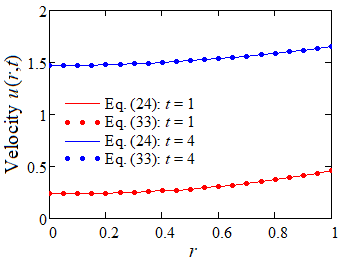
The inverse Laplace transform of Eq. (32), although quite difficult to get it, could be determined by the complex functions method. However, in order to compare it with the exact solution given by Eq. (24), we shall use the refined algorithm of Weidemann and Trefethen [33]. According to this algorithm the values of the inverse Laplace transform \(u(r,t)\) of \(\hat{u}(r,s)\) are given by the relation \[\label{GrindEQ__33_} u(r,t)=\frac{h\chi }{\pi {\kern 1pt} t} \sum _{k=-N}^{N}(ihk+1)\, e^{-\chi (ihk+1)^{2} } \hat{u}\left(r,\frac{\chi }{t} (ihk+1)^{2} \right), \tag{33}\] in which \[\label{GrindEQ__34_} h=-\frac{2\pi }{\ln (\varepsilon )} -\frac{\ln (\varepsilon )}{2\pi N^{2} } ,\, \, \, \chi =-\frac{[\ln (\varepsilon )]^{3} }{4\pi ^{2} N^{2} } ,\, \, \, N=-\frac{4\ln (\varepsilon )}{3\pi } \tag{34}\] and \(\varepsilon\) is the level of the precision machine (its value \(2.22\cdot 10^{-16}\) is mentioned by Garrappa et al. [34]). Figure 2 clearly shows the equivalence of the expressions of the dimensionless velocity field \(u(r,t)\) given by the relations (24) and (33).
The axial Couette flows of ECUCIBFs inside an infinite right circular cylinder are analytically investigated under the influence of a constant magnetic field acting perpendicular to the cylinder axis. The fluid does not slip on the cylinder surface. The finite Hankel transform and the Laplace transform are used to determine analytic expressions for the dimensionless velocity \(u(r,t)\) of the fluid and non-trivial shear stress \(\tau (r,t)\). In addition, writing the governing equation for velocity as a Bessel equation, a new analytic expression was obtained for the Laplace transform \(\hat{u}(r,s)\) of \(u(r,t)\).
To determine the numerical values of the velocity \(u(r,t)\) it is necessary to know the positive roots of the equation \(J_{0} (z)=0\). The determination of the values of these roots was done using the subroutine \("root(\cdot )"\) from the MathCAD software package. We specify that the equation \(J_{0} (z)=0\) has a unique root in each interval \(\left(\frac{(4n-1)\pi }{4} ,\frac{(4n+3)\pi }{4} \right),\; n=1,2,…\).
Therefore, the roots of transcendental equation \(J_{0} (z)=0\) are given by \(r_{n} =root\left(J_{0} (z),\; z,\; \frac{(4n-1)\pi }{4} ,\frac{(4n+3)\pi }{4} \right),\; n=1,2,…\).
Numerical simulations based on the analytic and semi analytic expressions (24) and (33), respectively, of the fluid velocity have been used to prepare Figure 2 when \(f(t)=1-\cos (t)\). This figure highlights an excellent agreement between the two solutions. Numerical results in the real domain, in the case of the equality (33), have been determined by means of (34) using the numerical algorithm formulated by Weidemann and Trefethen [33].
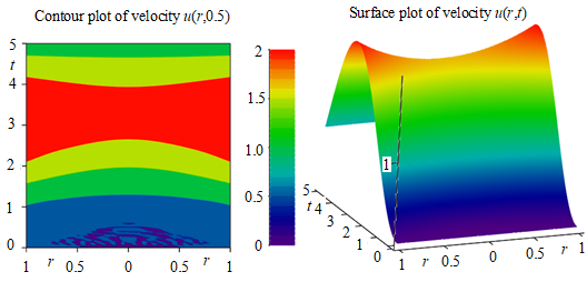
Figure 3 shows the contour plot and surface plot for the dimensionless velocity \(u(r,t)\) on the axial section of the cylinder, for the time interval \(t\in [0,5]\) corresponding to the cylinder velocity given by the same function \(f(t)=1-\cos (t)\). As expected, the fluid velocity has values symmetrical to the cylinder axis \(r=0\) and is significantly influenced by the boundary condition given by Eq. (12). For small values of time t the cylinder velocity is small and implicitly the fluid motion is slow. Once the values of time t increase, the fluid motion is achieved with higher values of the velocity reaching the maximum value on the cylinder surface, in the vicinity of the value 3 of time t. Obviously, the velocity field profiles will repeat after the time interval of length \(2\pi\) due to the periodicity of the function\(f(t)\).
Figures 4-6 were drawn for the boundary condition given by \(f(t)=2(1-e^{-t} )\). These figures show the contour plot and some profiles of the velocity \(u(r,t)\) on the axial section of the cylinder when some of the characteristic parameters of the fluid motion vary. More precisely, these figures analyze the effect of the magnetic parameter M, of the Burgers parameter \(\beta\) and of the relaxation time \(\alpha\). In all cases, the symmetry of the velocity \(u(r,t)\) with respect to the spatial variable r is evident.
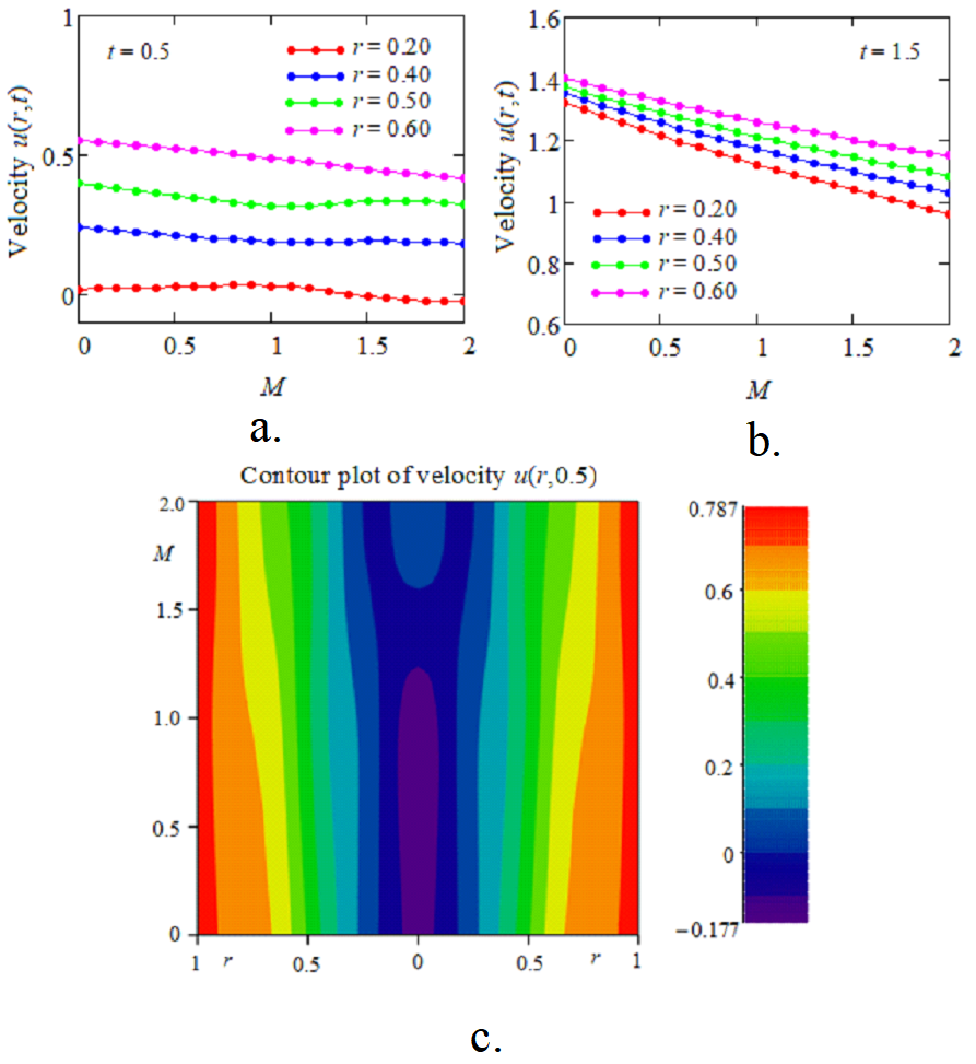
It can be observed from Figure 4 that for small values of the magnetic parameter M the fluid moves with a higher velocity than for large values of this parameter. This is due to the modification of the values of the Lorentz force which has a braking effect of the movement of fluid. Consequently, the fluid moves slower in the presence of a strong magnetic field. This property is explicitly shown in Figure 4c. For example, if \(M<1\), the fluid layers with velocity greater than 0.6 (orange and red colors) are much wider than the same layers for \(M>1\).
We should also note that for small values of time t there is reverse flow in the area adjacent to the cylinder axis, and the absolute value of the fluid velocity decreases with respect to the magnetic parameter M. On the other hand, Figure 4c highlights the fact that the fluid layers close to the cylinder surface move with higher velocities than the layers located further from this surface. This behavior is due to the fact that the fluid does not slip on the cylinder surface whose velocity significantly influences the velocities of the fluid in the layers close to the cylinder surface.
Figures 5 was drawn in order to highlight the effect of the dimensionless Burgers parameter \(\beta\) on the fluid velocity.
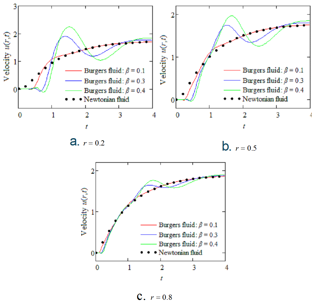
However, in order to have a comparison between the behavior of Newtonian and Burgers fluids, the time variations of the corresponding dimensionless velocities \(u(r,t)\) are together presented for three values of the parameter \(\beta\) at three different locations of the cylinder. The difference in behavior of the two fluids in this movement is clearly seen in these figures. As expected, it fades for increasing values of r and disappears near the cylinder. For small values of the \(\beta\) parameter and increasing values of the cylinder radius r, the velocity diagrams corresponding to the two fluids tend to overlap because the other two parameters have quite small values and their influence is negligible.
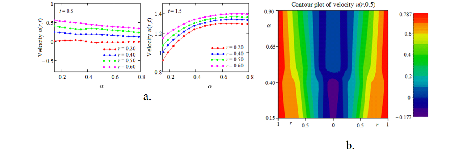
Figure 6 shows the influence of the \(\alpha\) dimensionless relaxation time on the fluid velocity. Figures 6a and 6b plot the fluid velocity profiles at different positions in the cylinder at two time points, namely \(t=0.5\) and \(t=1.5\), and Figure 6c shows the velocity contour plot at time \(t=0.5\), for values of the parameter \(\alpha\) in the range [0.15, 0.9].
For small values of this parameter, reverse flow of the fluid located in the central area of the cylinder is noticeable. For larger values of the relaxation time, the fluid in the central area moves quite slowly, and the fluid velocity increases in the area close to the cylinder boundary for all values of the \(\alpha\) non-dimensional relaxation time.
Finally, it is important to highlight the behavior of the fluid for large values of time t when the cylinder velocity tends to a constant value for \(t\to \infty\). Using the relations (A5) from Appendix A and Eq. (20) we obtain \[\label{GrindEQ__35_} {\mathop{\lim }\limits_{t\to \infty }} u(r,t)={\mathop{\lim }\limits_{s\to 0}} s\hat{u}(r,s)=c\, \left[1-2M\sum _{n=1}^{\infty }\frac{J_{0} (rr_{n} )}{r_{n} (r_{n}^{2} +M)J_{1} (r_{n} )} \right]=u_{s} (r), \tag{35}\] when \({\mathop{\lim }\limits_{t\to \infty }} f(t)=c\). In the same way from Eq. (26) it results that \[\label{GrindEQ__36_} {\mathop{\lim }\limits_{t\to \infty }} \tau (r,t)={\mathop{\lim }\limits_{s\to 0}} s\hat{\tau }(r,s)=2cM\sum _{n=1}^{\infty }\frac{J_{1} (rr_{n} )}{(r_{n}^{2} +M)J_{1} (r_{n} )} =\tau _{s} (r), \tag{36}\]
These important properties show that if the cylinder velocity has a finite limit as t tends to infinity, the fluid velocity \(u(r,t)\) and the corresponding shear stress \(\tau (r,t)\) tend to stationary values. Consequently, the fluid motion becomes steady in time. Furthermore, the velocity and shear stress fields \(u_{s} (r)\) and \(\tau _{s} (r)\) correspond both to Newtonian and non-Newtonian fluids. This is not a surprise because the governing equations corresponding to steady motions of these fluids are identical. As expected, direct computations show that \(u_{s} (r)\) and \(\tau _{s} (r)\) given by Eqs. (35) and (36), respectively, satisfy the corresponding governing equations.
In this work the axially symmetric motion problem of ECUCIBFs in an infinite circular cylinder that slides along its symmetry axis with the time-dependent velocity \(Vf(t)\) has been analytically and numerically investigated under the influence of a circular constant magnetic field that acts perpendicular to the symmetry axis of the cylinder. The fluid does no slip on the cylinder surface and two particular cases have been taken into consideration. The main results that have been here obtained are:
– Exact analytical expressions have been determined for the dimensionless fluid velocity \(u(r,t)\) and the corresponding non-zero shear stress \(\tau (r,t)\).
– For the results’ validation, the velocity \(u(r,t)\) has been presented in two different forms. Their equivalence when \(f(t)=1-\cos (t)\) was graphically proven in Figure 2.
– Numerical results from Figure 3 clearly highlight the axially symmetric aspect of the flow and the significant influence of the cylinder velocity on the fluid velocity.
– At small values of \(\alpha\)and of the time t a reverse flow of the fluid is noticeable in the central area of the cylinder. For larger values of the time t the fluid velocity grows up for increasing values of this parameter.
– Except a small vicinity of the symmetry axis of cylinder, the fluid flows slower in the presence of a magnetic field.
– If the function \(f(t)\) has a finite limit as t approaches infinity, the fluid velocity and the shear stress approaches the stationary solutions for large values of time t.
\((r,\theta ,z)\)– cylindrical coordinates
\(u(r,t)\) – axial velocity
T – the stress tensor
S – the extra-stress tensor
D the symmetric part of the velocity gradient
I – the identity tensor
p – the hydrostatic pressure
\(\mu\) – the fluid viscosity
\(\rho\) – the fluid density
\(\sigma\) – the electrical conductivity
\(\alpha\) – dimensionless relaxation time
\(\gamma\) – dimensionless retardation time
\(\beta\) – dimensionless Burgers parameter
M – dimensionless magnetic parameter
\(\tau (r,t)\) – the shear stress
\(J_{n} (\cdot )\) – standard Bessel functions
\(\delta (\cdot )\) – the Dirac delta function
\(G_{a,b,c} (t,d)\) – Lorenzo-Hartley G-function
\(r_{n}\) – positive roots of equation \(J_{0} (z)=0\)
\[w_{H} (r_{n} )=\int _{0}^{1}rw(r)J_{0} (rr_{n} ) dr,\, \, \, w(r)=2\sum _{n=1}^{\infty }\frac{J_{0} (rr_{n} )}{J_{1}^{2} (r_{n} )} w_{H} (r_{n} ), \tag{A1}\]
\[\int _{0}^{1}r\left[\frac{d^{2} w(r)}{dr^{2} } +\frac{1}{r} \frac{dw(r)}{dr} \right]J_{0} (rr_{n} ) dr=-r_{n}^{2} w_{H} (r_{n} )+r_{n} w(1)J_{1} (r_{n} ),\tag{A2}\]
\[L^{-1} \left\{\frac{s^{b} }{(s^{a} -d)^{c} } \right\}=G_{a,b,c} (t,d);\, \, \, Re(ac-b)>0,\, \, \, Re(s)>0,\, \, \, \left|\frac{d}{s^{a} } \right|<1,\tag{A3}\]
\[L^{-1} \left\{\frac{s}{s^{2} -a^{2} } \right\}=\cosh (at),\, \, \, L^{-1} \left\{\frac{a}{s^{2} -a^{2} } \right\}=\sinh (at),\tag{A4}\]
\[{{lim }_{t\to \infty }} f(t)={{lim }_{s\to 0}} s\hat{f}(s) \text{ if }\hat{f}(s)=L\left\{f(t)\right\}.\tag{A5}\]