
Adaptive mesh refinement (AMR) methods are robust numerical techniques widely employed in solving partial differential equations (PDEs) across various fields of physics and engineering, including solid and fluid dynamics, heat transfer, hyperbolic conservation laws, and convection-diffusion problems. Analytical solutions to these equations are often challenging or impossible to derive, particularly when the solutions exhibit complex features such as shock waves or rarefaction waves, which are difficult to resolve using uniform grids. AMR methods play a critical role in the advancement of numerical approaches for solving PDEs by enabling localized mesh refinement in regions requiring higher resolution. Conventional numerical methods typically employ a uniform discretization across the entire computational domain. In contrast, AMR techniques focus computational resources by concentrating mesh points in localized regions of interest, where higher resolution is needed. This targeted refinement enhances solution accuracy while reducing overall computational cost. AMR achieves this by applying finer meshes selectively within specific regions of the physical domain. Broadly, AMR strategies can be categorized into three types: \(h\)-refinement (mesh subdivision), \(p\)-refinement (increasing polynomial order), and \(r\)-refinement (node relocation). In this study, we utilize the \(r\)-refinement technique, also known as the moving mesh method (MMM), which involves adjusting the positions of existing grid points within a fixed mesh structure. This approach redistributes nodes from smoother regions to areas with steep solution gradients, following mesh adaptation principles. The main goal is to concentrate grid points in regions where the solution varies rapidly, thereby enhancing accuracy without increasing the total number of computational cells. To enable a comparative analysis, we also implement the \(h\)-refinement method in our relativistic models. Numerical results and error analysis are presented in the final section. Throughout the paper, we refer to the \(h\)-refinement as AMR and the \(r\)-refinement as MMM.
In recent decades, there has been growing research interest in AMR techniques for solving hyperbolic partial differential equations (PDEs). Among the early contributions to the development of MMM is the work by Harten and Hyman [1], introduced adaptive moving mesh methods (AMMMs) for one-dimensional hyperbolic conservation laws. Their method involved dynamically adjusting the mesh at each time step to improve resolution around shocks and contact discontinuities. This was achieved using a one-dimensional Godunov scheme, which effectively captured the evolving solution features by concentrating grid points where they were most needed. Building on earlier developments, Azarenok et al. [2] extended the Godunov method within a moving mesh framework to enhance both its accuracy and adaptability. Further advancements were made by Osher and Sanders, who proposed a local time-stepping technique for one-dimensional conservation laws. This approach was later refined by Tan et al. [3], who combined local time refinement with moving mesh strategies. Their method enabled the use of smaller time steps in regions with finer spatial resolution, thereby increasing computational efficiency while maintaining high accuracy in capturing complex solution features. Fazio and LeVeque [4] investigated the application of MMM to hyperbolic conservation laws using the Clawpack software framework. In a related study, Stockie, Mackenzie, and Russell [5] proposed a decoupled moving mesh approach based on the equidistribution principle, employing a moving mesh partial differential equation (MMPDE) formulation. Their work introduced a Godunov-type MMM that utilized a variety of monitor functions to effectively identify and resolve shocks and discontinuities across different regions of the solution domain. Wan-Lung and Tan applied a MMM to the Boussinesq equation, building on the framework developed in [6]. Tang and Tang [7] proposed a rezoning-based moving mesh strategy for solving one- and two-dimensional conservation laws. Their approach involved solving the physical PDEs on a uniform mesh during each time step, followed by a conservative interpolation procedure to project the solution onto the updated, adapted mesh. A similar methodology was adopted by Zegeling et al. [8] in the context of one-dimensional magnetohydrodynamics (MHD) problems, where they also conducted a comparative analysis of \(h\)– and \(r\)-refinement techniques in terms of performance and accuracy. Huang et al. [9] proposed a strategy in which the MMPDE is solved simultaneously with the underlying physical PDEs to directly govern mesh movement. A central aspect of this approach is the design and selection of monitor functions, which are critical for ensuring mesh quality and effective adaptivity. They have conducted extensive investigations into various monitor function formulations and analyzed their impact on the accuracy, robustness, and overall performance of moving mesh methods [10], [11], [12].
More recently, in [13], the Burgers-Schwarzshild model was analyzed using both AMR and MMM, with a comparison made between its behavior and that of the classical Burgers equation through these adaptive techniques. The Burgers-Schwarzshild model itself is also a scalar hyperbolic balance law that includes a mass parameter arising from the Schwarzshild metric element and was originally derived in [14] as a relativistic extension of the classical Burgers equation. In the present study, we follow a similar approach for the Burgers–FLRW model, which is also a relativistic model and a scalar hyperbolic balance law but involves a time scale parameter instead of a mass parameter due to the FLRW metric (see [15] for further details). This study shares several similar numerical features with the Burgers-Schwarzshild model, particularly in shock and rarefaction wave propagation, which exhibit almost the same behavior under adaptive mesh techniques. Particularly, the numerical simulations based on the MMM indicate that the optimal monitor and smoothing functions for the Burgers–FLRW models are almost identical to those for the Burgers–Schwarzshild model. We refer the reader to [13] for further detail.
In this work our primary focus is on applying the MMM to the numerical solution of the Burgers–FLRW equations and assessing its performance by comparing the results with those obtained via the AMR method. For the AMR computations, we employ the MPI–AMRVAC framework—a parallel, high-performance software package designed for solving hyperbolic partial differential equations [16– 18], with the AMR algorithm following the methodology developed in [19, 20]. For the MMM, we develop a separate implementation inspired by the moving mesh strategy proposed by Tang and Tang [7], which utilizes a conservative interpolation technique. A key distinction in our work is the presence of a source term in the Burgers–FLRW model equations, introducing additional numerical challenges not addressed in [7].
The paper is structured as follows. §2 introduces the general framework of scalar hyperbolic balance laws along with the relativistic Burgers FLRW equations. A finite volume discretization is then presented, using a MUSCL-type scheme to improve accuracy. §3 provides a brief description of the MMM algorithm. §4 reports numerical experiments for the Burgers–FLRW models on both uniform and adaptive meshes. The performance of the MMM under different monitor functions is examined, followed by a direct comparison of the MMM and AMR strategies. The numerical outcomes are further examined through an \(L^1\)–error analysis, which supports the comparative behavior observed for the two approaches. The paper concludes with a summary of the main findings and final remarks.
The types of models in the present paper are of the form \[\label{Gen-Burg} \partial_tv+\partial_rF(v,r)=S(v,r), \tag{1}\] where \(v\) is the unknown function, \(F\) is the flux and \(S\) is the source term. The homogeneous part of (1), neglecting the source term, can also be expressed in diagonal form as \[\label{Gen-Burg2} \partial_tv+\lambda(t,r)\,\partial_rv=0, \tag{2}\] where \(\lambda = \lambda (t,r)\) is the wave speed. The Eq. (1) with flux function \(F(v) = v^{2}/2\) and vanishing source term \(S = 0\) reduces to the classical Burgers equation, \[\label{IB} \partial_t v + \partial_r \left( \tfrac{v^{2}}{2} \right) = 0, \quad v = v(t,r), \quad t > 0, \quad r \in \mathbb{R}, \tag{3}\] which has played a central role in the development of shock-capturing methods in non-relativistic fluid dynamics. Recent work by LeFloch and his collaborators extends the Burgers and Euler equations to the setting of curved spacetime [14, 15, 21, 22]. In these works, the authors develop a geometric formulation of the relativistic models and present finite volume methods for their numerical approximation. More details on the construction of well-balanced finite volume schemes for cosmological fluid flows are given in [23] by Cao and the references therein. It is shown that the proposed schemes are well-balanced and are able to preserve and capture smooth steady-state solutions of the relativistic equations. In addition, error analysis and grid convergence for homogeneous solutions of these well-balanced schemes are studied in [15, 24]. These works include several numerical experiments based on the \(L^1\) -norm error, where numerical solutions are compared with highly resolved reference solutions.
The length element of the FLRW metric is described by \[g=-c^2dt^2+ a(t)^2 \left(\frac{dr^2}{1-kr^2}+r^2d\theta^2+ r^2\sin^2\theta d\varphi^2\right), \tag{4}\] where \(t\) is the time parameter, \(a(t)\) is a prescribed function, called the cosmic expansion factor, characterizes the expansion or contraction of the universe; \(c > 0\) is the speed of light, and \(k\in \{-1,0,1\}\) is a constant discrete parameter (curvature of space). In particular, the cosmic expansion factor is equal to \[a(t)=a_0\left(\frac{t}{t_0}\right)^{\alpha}>0,\] for some given \(t_0\) with the scale exponent \(\alpha >0\) and the scale factor \(a_0>0\). By normalizing \(a_0 = 1\) and \(t_0 = \pm 1\), the cosmic factor takes the form \[a(t)=|t|^{\alpha},\] where \(\alpha\) is the exponent parameter. In FLRW background, a typical choice of exponent parameter is \(\alpha=2/3,\) i.e. \(a(t)=|t|^{2/3}.\) Following [15], after normalizing \(c=1\), the balance law (1) takes the form \[\label{Bur-F1} \partial_tv+\partial_r\left(\frac{(1-kr^2)^\frac12}{a(t)}\frac{v^2}{2}\right)=-\frac{\dot{a}(t)}{a(t)} v \left(1-v^2\right) – \frac{kr}{a(t)} \frac{v^2}{2} (1-kr^2)^{-\frac12}, \tag{5}\] which is so-called Burgers-FLRW model. With \(\dot{a}(t) = \partial a(t)/\partial t\), the expression \(\dot{a}(t)/a(t)\) describes the universe’s expansion rate, known as the Hubble parameter and denoted by \(H(t)\). Depending on the value of \(k\), Eq. (5) takes one of three forms:
Burgers-FLRW model I (\(k=-1\)) : \[\label{Bur-F1.1} \partial_tv+\partial_r\left(\frac{(1+r^2)^\frac12}{a(t)}\frac{v^2}{2}\right)=- v \left(1-v^2\right) H(t) + \frac{r}{a(t)} \frac{v^2}{2} (1+r^2)^{-\frac12}. \tag{6}\]
Burgers-FLRW model II (\(k=0\)) : \[\label{Bur-F1.2} \partial_t v+\partial_r\left(\frac{1}{a(t)}\frac{v^2}{2}\right)=- v \left(1-{v^2}\right) H(t) . \tag{7}\]
Burgers-FLRW model III (\(k=1\)) : \[\label{Bur-F1.3} \partial_tv+\partial_r\left(\frac{(1-r^2)^\frac12}{a(t)}\frac{v^2}{2}\right)=-v \left(1-v^2\right) H(t) – \frac{r}{a(t)} \frac{v^2}{2} (1-r^2)^{-\frac12}. \tag{8}\]
An equivalent form of (5) can also be recovered by rewriting the left hand side of the Eq. (5) in non-conservative form by \[\label{Bur-F2} \partial_t v +\frac{(1-kr^2)^{\frac12}}{a(t)}\partial_r\left(\frac{v^2}{2}\right)= – v\, (1-v^2)\, H(t). \tag{9}\]
According to [15], due to the \(t\)-dependency of the variable coefficients \(a(t)\) and \(\dot{a}(t)\), there is no static solution of the Burgers-FLRW model (except \(v\equiv 0\)). Instead, there exists spatially homogeneous solutions described by \[v(t)=\frac{L}{\sqrt{ a(t)^2+L^2}} \in[-1,1], \qquad L \in \mathbb{R}.\]
Thus the FLRW background describes a homogeneous and isotropic cosmology. More particularly the following can be observed:
All spatially homogeneous solutions satisfy \(|v|<1.\)
The infinity limit for the homogeneous solutions on an expanding background is \(\underset{t\to \infty } {\lim}v(t)=0.\)
The limit for the homogeneous solutions on a contracting background is \(\underset{\begin{smallmatrix} t\to 0 & \\t<0 \end{smallmatrix}}{\lim} v(t)= \pm 1.\)
The cosmic expansion function \(a(t)\) determines the geometric background, which may be of either expanding or contracting type. For nonlinear hyperbolic equations of the form (1), shock wave solutions are well-defined only in the forward time direction. It is important to note that the Burgers–FLRW models (5)–(9) exhibit a singularity at \(t = 0\). Consequently, two formulations of the initial value problem may be considered, corresponding to the time intervals \(t \in [0,\infty)\) and \(t \in (-\infty,0]\). For the first case, \(t \in [0,\infty)\), the background represents an expanding universe, where \(a(t)\) increases monotonically toward \(+\infty\), and the initial data are prescribed at some positive time \(t_{0} > 0\). In the second case, \(t \in (-\infty,0]\), the background is contracting toward the future, with \(a(t)\) decreasing monotonically to \(a(0) = 0\), and the initial data are prescribed at a negative time \(t_{0} < 0\). Further details can be found in [25]. In this manuscript we consider the initial data for expanding universe, i.e. \(t \in [0,\infty)\).
In recent years, considerable attention has been given to the convergence analysis of finite volume methods for hyperbolic conservation laws in curved spacetime. LeFloch and collaborators have contributed extensively to this area, publishing studies on both the convergence and analytical properties of hyperbolic conservation laws, as well as on the formulation of relativistic models in curved spacetimes [14, 15, 21]. This study employs a finite volume framework, building on the approximation techniques developed in [14, 15, 21]. We consider the hyperbolic balance law (1) subject to a Riemann problem, with a piecewise constant initial data \[\label{Riem} v(0,r)=v_0(r)= \begin{cases} v_L, \quad r<c_0,\\ v_R, \quad r>c_0. \end{cases} \tag{10}\]
The temporal and spatial discretization is defined using two mesh sizes, \(\Delta t\) and \(\Delta r\), respectively. The discrete time levels are given by \[t_n= t_0+n\Delta t, \quad n=0,1,\cdots,\] while the spatial domain is discretized at the grid points \[r_j=j\Delta r, \qquad r_{j+1/2}=({j+1/2})\Delta r, \quad j=0,1,\cdots.\]
We set the approximation of solution \(v(t_n,r)\) over the grid cell \([r_{j-1/2},r_{j+1/2}]\) at time \(t_n\) and the initial data, respectively, as follows: \[v_j^n=\frac{1}{\Delta r}\int_{r_{j-1/2}}^{r_{j+1/2}} v(t_n,r) dr, \qquad v_j^0=\frac{1}{\Delta r}\int_{r_{j-1/2}}^{r_{j+1/2}} v(0) dr. \tag{11}\]
Integrating the balance law (1) on the rectangle \(R_{jn}=[r_{j-1/2},r_{j+1/2}]\times [t_n,t_{n+1}]\) yields the divergence form
\[\begin{aligned} \label{INT} \int_{r_{j-1/2}}^{r_{j+1/2}}v(t_{n+1},r) dr &= \int_{r_{j-1/2}}^{r_{j+1/2}}v(t_n,r) dr – \int_{t_n}^{t_{n+1}}F(v(t, r_{j+1/2}))dt +\int_{t_n}^{t_{n+1}}F(v(t, r_{j-1/2}))dt + \iint_{R_{jn}} S(t,r) dr\,dt. \end{aligned} \tag{12}\]
Dividing (12) by \(\Delta r\) gives \[\begin{aligned} \label{INT2} v_j^{n+1} &= v_j^n – \frac{\Delta t}{\Delta r}\left(\frac{1}{\Delta t} \int_{t_n}^{t_{n+1}}F(v(t, r_{j+1/2}))dt-\frac{1}{\Delta t}\int_{t_n}^{t_{n+1}}F(v(t, r_{j-1/2}))dt\right) + \frac{1}{\Delta r}\iint_{R_{jn}} S(t,r) dr\,dt. \end{aligned} \tag{13}\]
We proceed by defining the numerical flux, which approximates the physical flux function and is expressed as \[\begin{aligned} \label{INT3} \mathcal{F}_{j+1/2}^{n}= \frac{1}{\Delta t} \int_{t_n}^{t_{n+1}}&F(v(t, r_{j+1/2}))dt, \quad \mathcal{F}_{j-1/2}^{n}= \frac{1}{\Delta t}\int_{t_n}^{t_{n+1}}F(v(t, r_{j-1/2}))dt, \end{aligned} \tag{14}\] and the numerical source term as \[\label{INT3.1} \mathcal{S}_{j}^{n}= \frac{1}{\Delta r \Delta t}\int_{r_{j-1/2}}^{r_{j+1/2}}\int_{t_n}^{t_{n+1}} S(t,r) dr\,dt \approx \frac{1}{\Delta r}\int_{r_{j-1/2}}^{r_{j+1/2}} S(t_n,r) \,dr. \tag{15}\]
Finally, we arrive at the finite volume scheme, which takes the form \[\label{INT4} v_j^{n+1} = v_j^n- \frac{\Delta t}{\Delta x} \left(\mathcal{F}_{j+1/2}^{n}- \mathcal{F}_{j-1/2}^{n}\right) + \Delta t\mathcal{S}_{j}^{n}. \tag{16}\]
The value of the numerical flux \(\mathcal{F}_{j\pm 1/2}^{n}(v_{j\pm\frac12}^-,v_{j\pm\frac12}^+)\) and the numerical source term \(\mathcal{S}_{j}^{n}\) depend on the value of the physical flux \(F\) at the interfaces \(r_{j\pm 1/2}\), where \(v_{j+\frac12}^-\) and \(v_{j+\frac12}^+\) are the left and right states at an interface \(r_{j+ 1/2}.\) In this article the local Lax-Friedrichs flux functions \[\label{LLFF} \mathcal{F}(v_{j+\frac12}^-,v_{j+\frac12}^+)=\frac12 \left(F(v_{j+\frac12}^-)+ F(v_{j+\frac12}^+) – \max\limits_v\{ |F_v|\} (v_{j+\frac12}^+-v_{j+\frac12}^-)\right), \tag{17}\] are used for calculation of numerical flux. We then apply a MUSCL-type scheme proposed by Tang and Tang [7]. The fluxes at cell interfaces are computed by reconstructing the interface values \(v_{j\pm \frac12}\) from the cell-centered values of the adjacent left and right cells using
\[\begin{aligned} \label{MUSCL1}\begin{cases} v_{j+\frac12}^{+}&=v_{j+1}-\frac12(r_{j+\frac32}-r_{{j+\frac12}}) \, q_{j+1}\\\ v_{j+\frac12}^{-}&=v_j+\frac12(r_{j+\frac12}-r_{j-\frac12}) \, q_j.\end{cases} \end{aligned} \tag{18}\]
Here \(q_j\) is an approximation of the slope \(v_r\) at \(r_j\) defined by \[\label{MUSCL2} q_{j}=\left(\text{sign}(q_{j}^+)+\text{sign}(q_{j}^-)\right) \frac{|q_{j}^+ q_{j}^-|}{|q_{j}^+|+|q_{j}^-|}, \tag{19}\] with \[\label{MUSCL3}q_{j}^+=\frac{v_{j+1}^n-v_{j}^n }{r_{j+1} – r_{j}}, \qquad q_{j}^-=\frac{v_{j}^n-v_{j-1}^n }{r_{j} – r_{j-1}}. \tag{20}\]
By substituting (18) together with (19) and (20) into the local Lax-Friedrichs scheme (17), the numerical fluxes can be computed accordingly. As a result, the scheme (16) transforms into a MUSCL-type finite volume scheme with the local Lax-Friedrichs flux, which can then be solved iteratively.
To ensure the stability of the finite volume scheme (16), the CFL (Courant-Friedrichs-Lewy) condition \[\label{CFL0} \frac{\Delta t } {\Delta r} {\max_v} |\partial_v F(v,r)| \leq 1, \tag{21}\] must be satisfied for the general hyperbolic balance law (1). Thus, the CFL conditions for the the Burgers–FLRW Eq. (5) require \[\label{CFL1} \frac{\Delta t} {\Delta r} \underset{j}{\max}\Big|\frac{(1-k\,{r}_j^2)^{1/2}}{a(t_n)} \Big| |v_{j}^{n}| \leq 1. \tag{22}\]
The main idea of the MMM is to redistribute a fixed number of grid points, concentrating them in regions where the solution changes rapidly, thereby enhancing resolution in these areas. Once the mesh is adapted to the solution at a given time level \(t\), the solution is advanced to the next time level, \(t+\Delta t\), using the updated mesh. After this evolution step, the mesh is again adjusted to align with the newly computed solution. In this paper, we follow the approach proposed by Tang and Tang [7], employing a finite volume method to solve the relativistic model. Specifically, the numerical solution of the hyperbolic balance law in its general form (1) using an adaptive moving mesh technique is carried out in two main steps:
setting up the moving mesh through a mesh redistribution algorithm
solving the physical PDE on the adapted mesh.
Beyond the monitor function used in [7], this work investigates two additional monitor functions. Moreover, in addition to the low-pass filter form described in [7] and [8], we apply the weighted smoothing function proposed in [5] to increase mesh regularity. A comparison of numerical solutions obtained using the different monitor functions, along with the effect of smoothing, is presented in the last section.
The mesh generation equation is based on the equidistribution principle \[\label{EP} \left(\omega r_{\xi}\right)_{\xi} = 0, \quad \xi \in [0,1], \tag{23}\] where \(\omega\) is a monitor function, \(r\) and \(\xi\) denote the physical and computational coordinates, respectively. The monitor function generally depends on the solution and is typically expressed in terms of spatial derivatives of \(v\). It serves as an indicator of the solution’s complexity, identifying regions with steep gradients or singularities and directing the adaptive placement of mesh points. The Eq. (23) is solved in the computational domain \([0, 1]\) with a uniform mesh. After obtaining the new mesh {\(\tilde{r}_j\)} by (23), we update the numerical solution on the new points \(\tilde{r}_{j}= {\tilde{r}_{j-\frac12}+\tilde{r}_{j+\frac12}}/2\). According to [7], a second-order conservative interpolation formula preserves total variation, ensuring that the resulting adaptive mesh solutions retain the fundamental properties of hyperbolic conservation laws. For the Burgers-FLRW models, we use the same conservative interpolation formula given by \[\label{Con-mesh1} \Delta \tilde{r}_{j} \, \tilde{v}_{j} = \Delta r_{j} \, v_{j} – \left( (cv)_{j+\frac{1}{2}} – (cv)_{j-\frac{1}{2}} \right), \tag{24}\] where \[\label{Con-mesh1.0} \Delta \tilde{r}_{j} = \tilde{r}_{j+\frac{1}{2}} – \tilde{r}_{j-\frac{1}{2}}, \qquad c_{j+\frac{1}{2}} = r_{j+\frac{1}{2}} – \tilde{r}_{j+\frac{1}{2}}. \tag{25}\]
The numerical solution \(\tilde{v}\) at the adapted mesh points \(\tilde{r}_{j+\frac{1}{2}}\) is computed based on the solution values \(v_j\) on the original mesh and the corresponding mesh locations \(r_{j+\frac{1}{2}}\), thereby ensuring a consistent transfer of information between the old and new meshes. In the actual computation, the linear flux \(c\nu\) is approximated by \[\label{Con-3.0} (cv)_{j+\frac{1}{2}} = \frac{c_{j+\frac{1}{2}}}{2} \left( v_{j+\frac{1}{2}}^+ + v_{j+\frac{1}{2}}^- \right) – \frac{|c_{j+\frac{1}{2}}|}{2} \left( v_{j+\frac{1}{2}}^+ – v_{j+\frac{1}{2}}^- \right), \tag{26}\] where \(v_{j+\frac{1}{2}}^+\) and \(v_{j+\frac{1}{2}}^-\) denote the reconstructed values of \(v\) at the interface \(r_{j+\frac{1}{2}}\) from the right and left sides, respectively. These are approximated using the MUSCL-type reconstructions given in (18)–(20).
The moving mesh strategy employed in this work follows the framework introduced in [7]. It integrates an iterative mesh adaptation procedure guided by the equidistribution principle (23) with a conservative solution interpolation technique (24). To advance the solution in time, a MUSCL-type finite volume scheme with a local Lax–Friedrichs flux is applied, providing both accuracy and numerical stability. The overall algorithm can be summarized as follows:
Grid Initialization
Generate an initial uniform computational grid over the domain.
Compute the initial physical mesh points \(\{ r_j^{[0]} \}\) by enforcing the equidistribution condition (23) on the initial data.
Iterative Mesh Adaptation and Conservative Interpolation
Evaluate the cell-averaged values of the initial condition, \(\{ v_{j+\frac{1}{2}}^{[0]} \}\), on the current mesh.
Update the mesh positions \(\{ r_{j+\frac{1}{2}}^{[\nu]} \}\) via iterative solution of the discretized equidistribution equation: \[\label{eq:redistribution} \omega(v_{j+1}^{[\nu]}) \left( r_{j+\frac{3}{2}}^{[\nu]} – r_{j+\frac{1}{2}}^{[\nu+1]} \right) – \omega(v_j^{[\nu]}) \left( r_{j+\frac{1}{2}}^{[\nu+1]} – r_{j-\frac{1}{2}}^{[\nu+1]} \right) = 0, \tag{27}\] using a Gauss–Seidel iteration scheme. The monitor function \(\omega\) captures local solution features.
Interpolate the solution \(\{ v_{j+\frac{1}{2}}^{[\nu]} \}\) conservatively onto the updated mesh \(\{ r_{j+\frac{1}{2}}^{[\nu+1]} \}\), yielding the new solution values \(\{ v_j^{[\nu+1]} \}\).
Repeat steps (b) and (c) until convergence is achieved, determined either by the satisfaction of the tolerance condition \[\| r^{[\nu+1]} – r^{[\nu]} \| \leq \epsilon,\] where \(\epsilon\) is a prescribed small positive value, or by reaching a predefined maximum number of iterations.
Temporal Solution Update
Advance the numerical solution from \(t^n\) to \(t^{n+1}\) using a MUSCL-type finite volume scheme with a local Lax–Friedrichs flux, applied on the adapted mesh \(\{ r_j^{[\nu+1]} \}\). This results in the updated solution values \(\{ v_j^{n+1} \}\).
Time Marching Procedure
If \(t^{n+1} \leq T\), update the initial values for the next time step: \[v_j^{[0]} \leftarrow v_j^{[\nu+1]}, \quad r_j^{[0]} \leftarrow r_j^{[\nu+1]},\] and return to Step 2 to begin the next time iteration.
In the literature, the most widely used monitor functions include arc-length-based, curvature-based, and optimal monitor functions. In this work, we focus on the following monitor functions:
Arc length based monitor function with a constant choice of \(\alpha\) \[\label{Arc} \omega= \sqrt{1+\alpha\, |v_{r}|^2} \quad {\text{where}} \quad \alpha = constant. \tag{28}\]
Arc length based monitor function with solution dependent parameter \(\alpha_{avg}\) \[\label{Arca} \omega= \sqrt{1+\frac{1} {\alpha_{avg}}\, | v_{r}|^2} \quad \mbox{ where } \quad \alpha_{avg} =\frac{1}{|r_{max}-r_{min}|} \int_{r_{min}}^{r_{max}}|v_r|^2dr. \tag{29}\]
Shock monitor function \[\label{Shock} \omega= \sqrt{1+\beta \left( \frac{|v_{r}|}{\max_r|v_{r}|}\right)^2} \quad \mbox{ where } \quad \beta = const. \tag{30}\]
In addition, to enhance mesh regularity, two complementary smoothing techniques are applied to the computed monitor function:
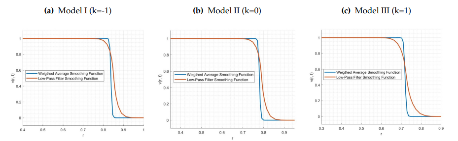
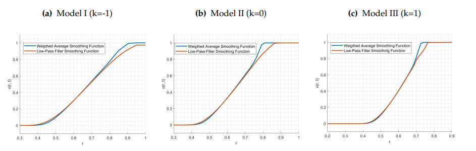
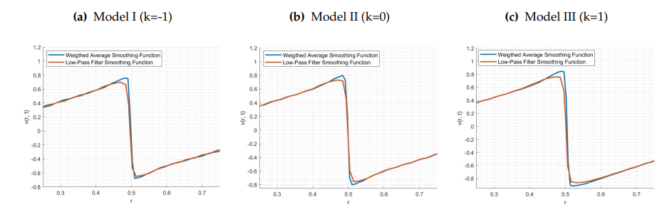
Low-pass filter smoothing: \[\label{lowpass} \omega_{j}^{\mathrm{smooth}} = \frac{1}{4}\left(\omega_{j+1} + 2\omega_{j} + \omega_{j-1}\right), \tag{31}\]
Weighted average smoothing: \[\label{weighted} \omega_j^{\mathrm{smooth}} = \sqrt{ \frac{ \sum_{k=j-i_p}^{j+i_p} \omega_k^2 \left(\frac{\gamma_s}{1+\gamma_s}\right)^{|k-j|} }{ \sum_{k=j-i_p}^{j+i_p} \left(\frac{\gamma_s}{1+\gamma_s}\right)^{|k-j|} } }. \tag{32}\]
The smoothing procedures are applied iteratively after each update of the monitor function to maintain mesh regularity and prevent grid irregularities. The low-pass filter method (31), used in [7] and [8], has been shown to produce smooth meshes effectively. In contrast, the weighted average smoothing technique (32), proposed in [5], provides a more localized and adaptive smoothing effect. In this study, both methods are systematically evaluated, and, as shown in Section 4, the weighted average smoothing consistently yields superior results across a range of numerical experiments for the Burgers–FLRW models.
Our numerical experiments are divided into two main categories. The first category examines the governing equations on uniform, non-adaptive meshes. The second, and primary, category focuses on results obtained using the MMM approach. In addition, numerical results obtained via the AMR technique, implemented through the MPI-AMRVAC framework, are included to enable a comparative study with MMM. For MMM, a MATLAB code is developed to perform dynamic mesh redistribution and generate supplementary numerical results. A detailed comparative analysis is then carried out to assess the effectiveness of these two adaptive approaches across the relativistic models.
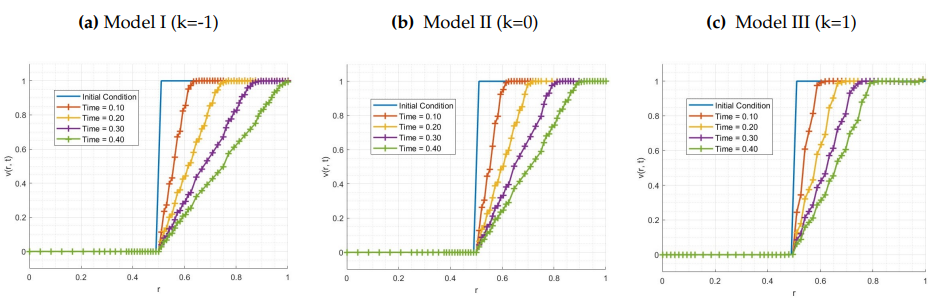
Our numerical experiments begin with finite volume discretizations of the models (6)–(8) on a fixed uniform mesh. The aim of this chapter is to observe the behavior of models in their simplest form using three different initial conditions, which is necessary to understand the development of shock and rarefaction waves over time.
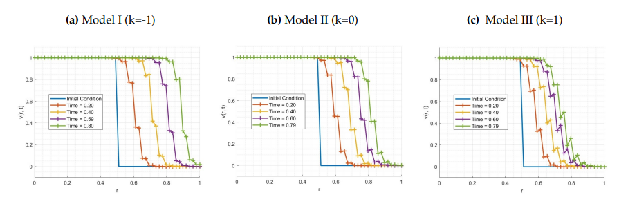
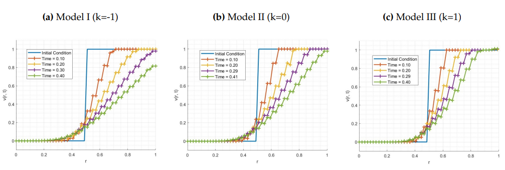
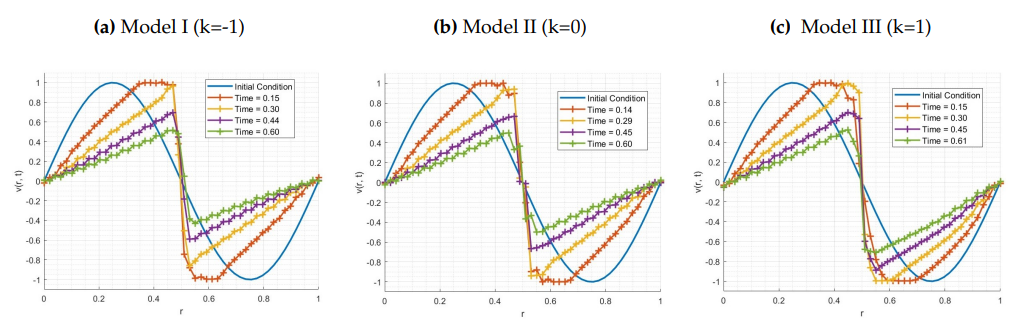
The initial conditions are given by \[ v_0(r) = \begin{cases} 1, r < 1/2, \\ 0, r > 1/2, \end{cases} \qquad \text{(IC1: shock wave)}, \label{IC.1} \tag{33}\] \[v_0(r) = \begin{cases} 0, r < 1/2, \\ 1, r > 1/2, \end{cases} \qquad \text{(IC2: rarefaction wave)}, \label{IC.2} \tag{34}\] \[v_0(r) = \sin(2\pi r), \quad 0 \leq r \leq 1 , \qquad \text{(IC3: smooth data)}. \label{IC.3} \tag{35}\]
The simulations on the uniform mesh are conducted with \(J = 50\) grid points and a CFL number of 0.7 to ensure numerical stability. For FLRW Models I, II, and III, the curvature parameter \(k\) is assigned the values \(-1\),\(0\) and \(1\) respectively. The computational domain is defined as \(r \in [r_{\min}, r_{\max}]=[0,1]\). A MUSCL-type finite volume scheme incorporating a minmod limiter is employed to achieve non-oscillatory reconstruction of the solution. In all uniform mesh simulations, noticeable oscillations arise during the propagation of shock and rarefaction waves, affecting both smooth and piecewise-smooth initial data. These oscillations are particularly appeared around and after the jump point \(r = 1/2\), as illustrated in Figures 1–3.
These observations are consistent with the findings of Dubey and Biswas [26], who conducted a detailed study of numerical oscillations in Lax–Friedrichs-type schemes. Their simulations of the Burgers and linear advection equations reveal similar oscillatory patterns near jump discontinuities. To mitigate such oscillations, they propose a hybrid approach incorporating an upwind scheme. Because our finite volume solver also uses a Lax–Friedrichs flux, the oscillations observed in simulations of relativistic models are consistent with the findings in [26]. These oscillations could be reduced on a uniform grid by using alternative fluxes, such as the Godunov-type methods suggested in [27], which provide better resolution of discontinuities. However, instead of changing the flux function, we show in the following subsection that applying adaptive techniques can effectively suppress these oscillations. In particular, combining our MUSCL-type scheme with a local Lax–Friedrichs flux and adaptive mesh strategies produces oscillation-free results for our relativistic models. Which is a clear advantage of adaptive mesh approaches in enhancing solution quality and stability compared to fixed uniform meshes.
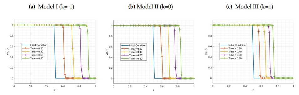
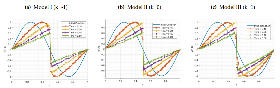
This section begins with the presentation of the numerical solution computed on an adaptive mesh refined with the AMR approach using the MPI–AMRVAC framework. Subsequently, the section then focuses on MMM and identifying the most suitable monitor and smoothing functions for the Burgers-FLRW models, chosen among the functions defined in Eqs. (28)–(32).
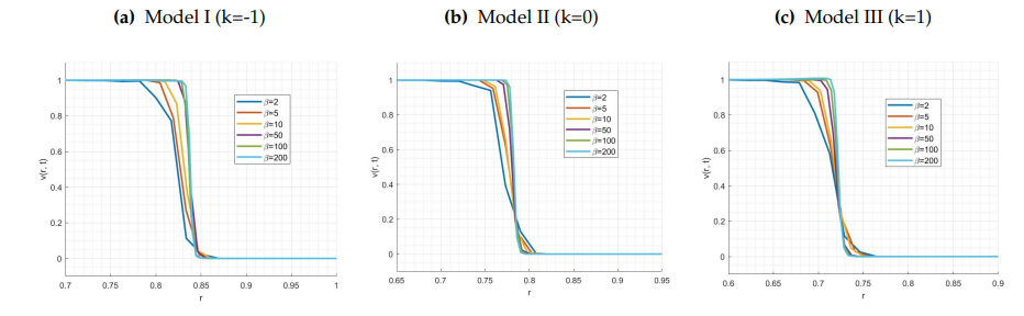
Figures 4-6 are numerical solutions of (6)–(8), calculated by MPI-AMRVAC, a parallel framework for hyperbolic PDEs [16, 17], following the strategies in [19] which are based on AMR. This framework, initially discretizes the computational domain using a uniform mesh, and adaptively refines the existing mesh by dividing it into smaller subcells based on predefined refinement criteria. Depending on the allowed subdivisions, a maximum resolution of \(2^{m-1}\) can be achieved in the critical regions, where \(m = 4\) is used in our AMR tests. Moreover, the framework performs cell coarsening in regions where the solution exhibits smooth behavior and high spatial resolution is unnecessary. By dynamically performing cell refinement and coarsening, the AMR technique adaptively conforms the computational mesh to the underlying solution features, with enhanced resolution particularly concentrated near discontinuities. In our numerical experiments the average number of grid points denoted \(J_{\text{avg}}\), is used to characterize the adaptive mesh, as both the total number of points and simulation runtime may vary.
The numerical tests use an average number of grid points \(J_{\text{avg}}\) in the range \(40 \leq J_{\text{avg}} \leq 64\), with a CFL number of \(0.7\) for stability. The parameter \(k\) is set to \(k = 0\), the computational domain is \([r_{\min}, r_{\max}] = [0, 1]\), and the initial conditions IC1, IC2, and IC3 are given by Eqs. (33)–(35).
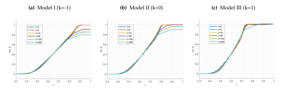
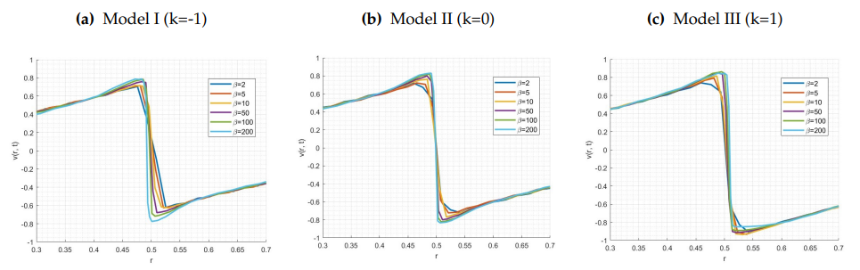
In Figures 4–6, each set of subfigures shows shock or rarefaction wave propagation for Model I (\(k=-1\)) on the left, Model II (\(k=0\)) in the middle, and Model III (\(k=1\)) on the right.
Figure 4 shows a shock wave from IC1, with similar wave structures across the Burger-FLRW models. Figure 5 presents a rarefaction fan from IC2, and Figure 6 depicts an \(N\)-wave shock from the sinusoidal IC3. In all cases, the solutions for IC1–IC3 are qualitatively similar across the three models. However the main observed effect of parameter \(k\) is a change in the wave propagation speed.
Our study integrates the method described by [7] with various smoothing and monitor functions present in the literature. A set of three monitor functions is selected to be investigated: arc length (28), solution-dependent arc length (29) and shock monitor (30), combined with low-pass (31) or weighted average (32) smoothing functions.
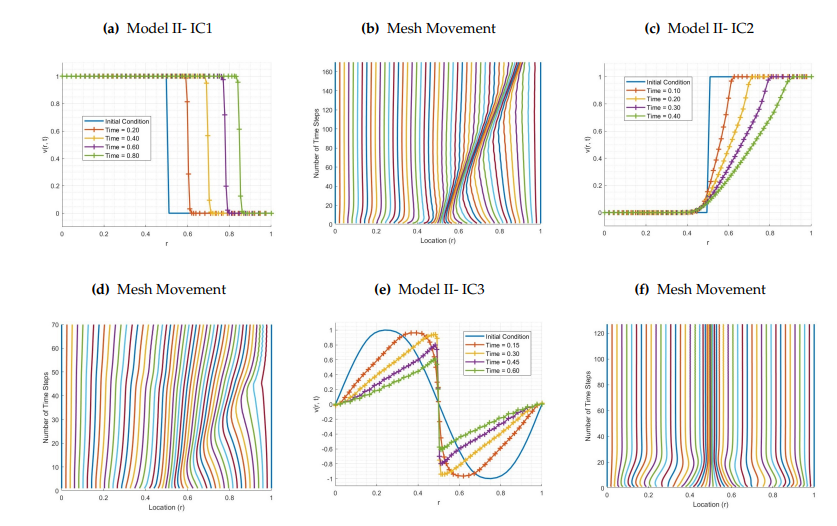
We observed that the efficiency of the monitor functions is identical across all three Burgers-FLRW models. Thus, we only present the results for Model II to select the most efficient monitor function, as shown in Figures 7–12. The shock monitor enhanced with weighted smoothing offers the most optimal performance, maintaining sharp shock profiles and reducing the number of time steps needed to reach \(t=1\). The arc-length monitor function with a solution-dependent value of \(\alpha\) does not require user-defined parameters and yields the sharpest shock profiles. However, this monitor function significantly reduces cell sizes, leading to an increased number of time steps.
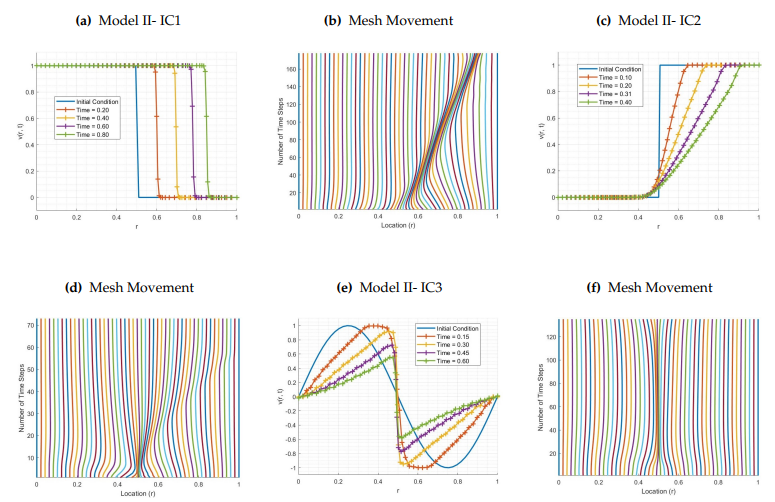
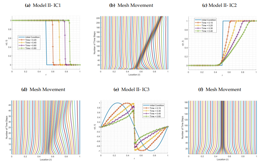
The shock monitor requires tuning of the constant \(\beta\), which controls shock and rarefaction resolution. Figures 9–11 illustrate the results of numerical experiments conducted to determine the optimal value of \(\beta\) for initial conditions IC1–IC3, corresponding to final times of \(t = 0.6\), \(0.3\), and \(0.45\), respectively. Results indicate that for IC1, increasing \(\beta\) sharpens discontinuities, where optimal interval is \(10 \le \beta \le 50\). For IC2, smaller \(\beta\) values (\(2 < \beta < 10\)) are better for rarefaction resolution. Finally, for IC3, a value of \(\beta = 50\) is found to optimally capture discontinuities while avoiding excessive refinement. Across all cases, the shock monitor performs most effectively within \(\beta \in [10, 50]\).
Following the determination of optimal \(\beta\) values, we investigate the effect of smoothing functions on mesh regularity. The low-pass filter (31) and weighted average (32) smoothing functions are applied to IC1–IC3. Figures 13–15 show the comparative results. For IC1, weighted average smoothing significantly improves computational efficiency compared to the low-pass filter. For IC2, both smoothing techniques produce nearly identical results. For IC3, the weighted smoothing again yields superior accuracy. These results confirm that the combination of shock monitor and weighted average smoothing provides the most robust and accurate outcomes for Burgers–FLRW models.
In conclusion, MUSCL-type finite volume schemes with adaptive meshes-AMR or MMM—substantially increase solution quality and stability compared to uniform grids. Within the MMM framework, the shock monitor combined with weighted average smoothing ensures optimal resolution of shock waves across all tested initial conditions for Burgers–FLRW models.
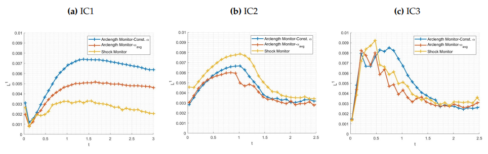
In addition to the qualitative analyses presented in the previous sections, this section discusses the results of a quantitative assessment based on the \(L^1\)–error norm. The results shown in Figures 16 and 17 were obtained by comparing the numerical solutions with a reference solution computed on a uniform grid consisting of 5000 cells for Model III (\(k = 1\)).
In contrast to previous experiments, the number of moving cells is set to \(J=200\). Using a smaller number of cells is observed to produce oscillatory behavior in the error norm, primarily due to the discrete relocation of the shock wave between adjacent cells. Increasing the number of cells mitigates this effect and yields a more stable error profile. However, refining the mesh also amplifies the maximum value of the first spatial derivative \(u_x\) particularly for IC1 and IC2, both of which exhibit shock-type behavior. These initial conditions are therefore susceptible to the over-refinement phenomenon, since the employed monitor functions depend directly on \(u_x\). Near shock locations, \(u_x\) grows unbounded, which may lead to excessive mesh concentration.
To control this effect, the parameters of the weighted average smoothing function were adjusted to \(i_p=32\) and \(\gamma_s=9\). This modification effectively regularizes the influence of large gradients and stabilizes the mesh adaptation process in the vicinity of shocks.
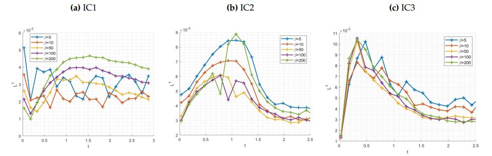
Figure 16 illustrate the evolution of the \(L^1\)–error norm over time for different monitor functions. The results supports the conclusion in the previous section, indicating that the shock monitor function provides the most accurate representation of shock profiles among the considered alternatives. When the shock monitor is used, the solution achieves relatively small \(L^1\)-error norms for IC1 and IC3, demonstrating its superior performance in capturing sharp gradients and discontinuities.
On the other hand, the arclength monitor function with \(\alpha_{avg}\) exhibits improved performance in simulations involving rarefaction-type behavior. Its formulation appears better suited to resolving smoothly varying solution structures, leading to enhanced accuracy in such cases.
For IC3, which involves a combination of shock and rarefaction characteristics, the performances of those two functions are comparatively close. The mixed nature of the solution profile reduces the distinct advantage observed in the pure shock or rarefaction scenarios.
Finally, the arclength monitor function with a constant \(\alpha\) parameter yields satisfactory results overall; however, it remains slightly inferior to the other two monitor functions in terms of accuracy and error reduction.
Before proceeding to the comparison of AMR and MMM, an investigation was conducted to assess the effect of the parameter \(\beta\) on the \(L^1\) error, with the aim of optimizing the shock monitor function. Figure 17 illustrates the evolution of the \(L^1\) error norm for different \(\beta\) values throughout the simulation. All data were obtained under identical simulation conditions as used in Figure 16.
The results shown in the figures are consistent with the conclusion reported in the previous section, indicating that \(\beta\) should be maintained within the range \(10 \leq \beta \leq 50\). When \(\beta\) is below 10, the \(L^1\) error increases across all three initial conditions, suggesting insufficient resolution. In contrast, \(\beta\) values above 50 lead to an increase in the \(L^1\) error for IC1, while producing no measurable improvement in accuracy for IC2 and IC3. In addition, larger \(\beta\) values primarily result in over-refinement, which reduces computational efficiency without providing corresponding gains in solution accuracy.
Both Figures 16 and 17 illustrate the behaviour of the \(L^1\) norm over time. The error norm exhibits a rapid increase at the beginning of the simulation, followed by a decrease and stabilization at a nearly constant value for the remainder of the simulation. This behaviour is consistent with the results reported by Sanjoyo et al. [28].
In the final phase of this study, the numerical performance of AMR and MMM techniques is investigated for the Burgers-FLRW models. Using the optimal shock monitor function and weighted smoothing, MMM simulations are conducted in MATLAB, while AMR method solutions are provided by MPI-AMRVAC.
Figures 18- 19 and Table 1 summarize computational times for different initial conditions. Simulation times for IC1, IC2, and IC3 are set to \(t=1\) for all models. Elapsed time values for AMR are normalized to MATLAB-equivalent performance using a factor of 6.9, based on prior comparisons between MPI-AMRVAC and MATLAB [8].
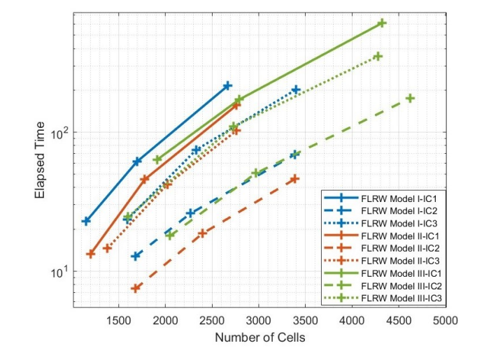
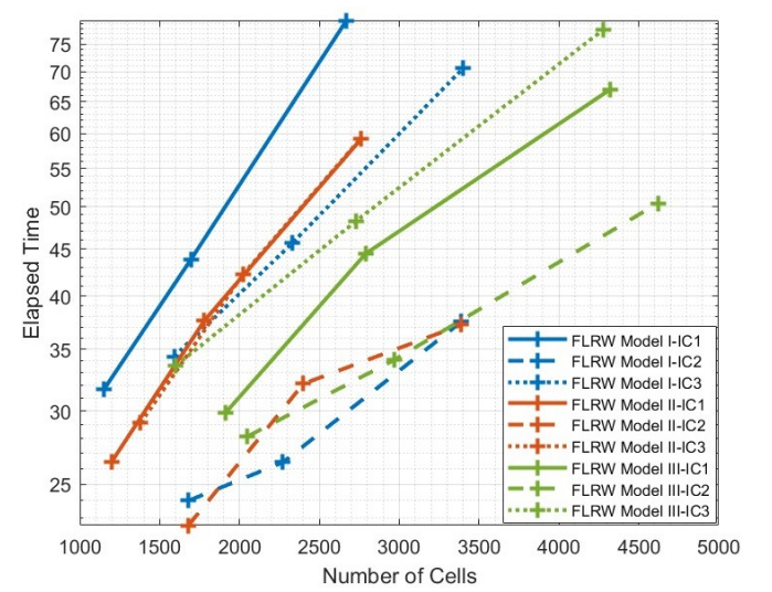
The results indicate that shock-type initial conditions lead to the longest computation times, whereas rarefaction waves develop smoothly and require fewer time steps to reach the final simulation time. This is due to discontinuities in the solution which require smaller cells and time steps as a result of the CFL condition.Problems with IC1 and IC3 require approximately the same computational time to reach the solution; however, IC3 is slightly faster due to the initial smoothness of the sine wave, which demands less mesh refinement in the beginning compared to the sharp shock wave present in IC1.
Solution times for MMM increase substantially with the number of cells, while AMR exhibits lower sensitivity to cell number due to its dynamic mesh adaptation.For a moderate number of grid cells, MMM demonstrates higher computational efficiency; however, at high resolutions, the AMR method becomes significantly faster. For instance, with FLRW Model II with IC1, and approximately 2760 cells, AMR requires 59.16 seconds versus 156.09 seconds for MMM, highlighting the stronger dependence of MMM on grid size.
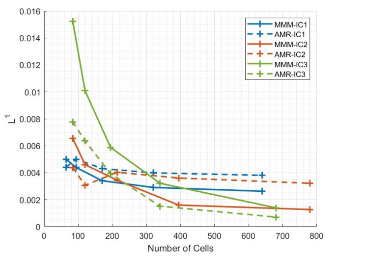
On the other hand, the results shown in Figure 20 provide a complementary perspective on the comparison between the two mesh refinement methods. The graph of \(L^1\) error versus the number of computational cells indicates that the MMM method compensates for its higher computational cost through increased accuracy, particularly when a large number of cells is employed. In contrast, the AMR method achieves satisfactory accuracy even with a relatively small number of cells. As the number of cells increases, the MMM method is more strongly affected than the AMR method, ultimately reaching a higher level of accuracy. The observed trade-off between computational time and solution accuracy highlights a balance between the two approaches.
For comparable setups (CFL, grid points, and initial conditions), as illustrated in Figures 4–12, MMM yields smoother solutions for shock and rarefaction waves by more efficiently mitigating the oscillations discussed in §4.2. Across all cases, the comparison indicates that MMM excels at resolving oscillations, while AMR offers competitive performance for large-scale computations.
Our study presented numerical solutions for the relativistic Burgers FLRW model with different initial conditions and compared the performance of two distinct adaptive mesh methods. The first method used was adaptive mesh refinement (AMR), which dynamically adjusts the computational mesh to the features of the underlying solution by subdividing or coarsening the grid cells. The second approach, the Moving Mesh Method, adapts the computational grid by relocating existing nodes to regions requiring higher resolution while maintaining a constant total grid points.
Numerical experiments involving the AMR approach were conducted using the MPI-AMRVAC framework, which provides dynamic mesh refinement capability. The MMM was implemented through a custom MATLAB script, in which the mesh dynamics are regulated by the application of chosen monitor and smoothing functions. Based on numerical experiments and evaluations, following conclusions are deduced.
Accurate solutions of the Burgers-FLRW models with different initial conditions were obtained using AMR and MMM adaptive mesh approaches.
MPI-AMRVAC, which is a parallel processing software designed for solving hyperbolic PDEs (https://amrvac.org), was utilized to implement the AMR approach.
The Lax–Friedrichs flux scheme, when applied on a uniform mesh, produces oscillatory solutions for the Burgers-FLRW models. AMR and MMM techniques mitigate these oscillations and yield smoother solution profiles.
Our study integrates Tang and Tang’s framework [7] with a variety of monitor and smoothing functions, and subsequently proposes a modified moving mesh method that employs the most effective combination to solve Burgers-FLRW models.
Different combinations of monitor and smoothing functions were tested to determine the optimal configuration for the MMM method. The shock monitor function (30) combined with the weighted average smoothing method (32), as presented by Stockie et al. [5], proved to be the most suitable choice for Burgers-FLRW equations, as it offers optimal performance by balancing accuracy and computational efficiency.
Selecting the appropriate value for the parameter \(\beta\) is crucial for solution accuracy, as higher values improve shock resolution, while lower values are better suited for capturing rarefaction waves.
Over-refinement of the mesh causes an increased iteration count to reach the final simulation time; hence, careful selection of the \(\beta\) parameter and monitor function is essential to achieve best computational efficiency.
Comparative study between AMR and MMM reveals the effects of grid size and initial condition to accuracy and computational efficiency. Our study indicates that the MMM approach offers faster computations when a small number of grid points is utilized, whereas AMR becomes advantageous in terms of speed in simulations involving a higher number of grid points.
The MMM method is more sensitive to changes in grid size. By decreasing the grid size, the MMM method achieves higher accuracy compared to the AMR method, while requiring increased computational time.
The adaptive mesh techniques presented in this study can be extended to two-dimensional relativistic systems.
The data that support the findings of this study are available from the authors upon request.
The first author was supported by TUBITAK 2219 Project 2023/1 through the grant “Project No: 1059B192301367”.
Table 1 presents the elapsed time required to solve different types of problems using both AMR and MMM. The first column lists the test equations along with their respective initial conditions (IC1, IC2, or IC3) and the average number of grid points, Javg. The second column shows the computation time for each test case using the AMR approach implemented in MPI-AMRVAC. A MATLAB equivalent of the result in the second column is provided in the third column. The final column reports the computation time for each test case using the MMM.
| Test Case | AMR MPI-AMRVAC (s) | AMR MATLAB Equivalent(s) | MMM MATLAB (s) |
| FLRW Model I-IC1 \(J_avg\)=1150 | 4.59 | 31.66 | 22.75 |
| FLRW Model I-IC1 \(J_avg\)=1695 | 6.35 | 43.80 | 61.33 |
| FLRW Model I-IC1 \(J_avg\)=2670 | 11.54 | 79.60 | 216.27 |
| FLRW Model I-IC2 \(J_avg\)=1680 | 3.48 | 23.99 | 12.79 |
| FLRW Model I-IC2 \(J_avg\)=2270 | 3.83 | 26.40 | 26.04 |
| FLRW Model I-IC2 \(J_avg\)=3390 | 5.44 | 37.52 | 69.18 |
| FLRW Model I-IC3 \(J_avg\)=1590 | 4.99 | 34.40 | 23.42 |
| FLRW Model I-IC3 \(J_avg\)=2330 | 6.61 | 45.63 | 74.64 |
| FLRW Model I-IC3 \(J_avg\)=3400 | 10.24 | 70.62 | 202.79 |
| FLRW Model II-IC1 \(J_avg\)=1200 | 3.83 | 26.45 | 13.32 |
| FLRW Model II-IC1 \(J_avg\)=1780 | 5.45 | 37.62 | 45.72 |
| FLRW Model II-IC1 \(J_avg\)=2760 | 8.57 | 59.16 | 156.09 |
| FLRW Model II-IC2 \(J_avg\)=1680 | 3.27 | 22.56 | \quad7.46 |
| FLRW Model II-IC2 \(J_avg\)=2400 | 4.66 | 32.13 | 18.68 |
| FLRW Model II-IC2 \(J_avg\)=3390 | 5.39 | 37.22 | 46.08 |
| FLRW Model II-IC3 \(J_avg\)=1380 | 4.22 | 29.13 | 14.59 |
| FLRW Model II-IC3 \(J_avg\)=2020 | 6.11 | 42.17 | 42.02 |
| FLRW Model II-IC3 \(J_avg\)=2760 | 8.59 | 59.30 | 102.51 |
| FLRW Model III-IC1 \(J_avg\)=1910 | 4.33 | 29.85 | 63.26 |
| FLRW Model III-IC1 \(J_avg\)=2790 | 6.44 | 44.46 | 171.69 |
| FLRW Model III-IC1 \(J_avg\)=4320 | 9.71 | 66.96 | 610.24 |
| FLRW Model III-IC2 \(J_avg\)=2050 | 4.08 | 28.17 | 17.94 |
| FLRW Model III-IC2 \(J_avg\)=2970 | 4.94 | 34.11 | 50.63 |
| FLRW Model III-IC2 \(J_avg\)=4620 | 7.31 | 50.42 | 175.20 |
| FLRW Model III-IC3 \(J_avg\)=1600 | 4.87 | 33.60 | 24.55 |
| FLRW Model III-IC3\(J_avg\)=2730 | 6.99 | 48.24 | 109.94 |
| FLRW Model III-IC3 \(J_avg\)=4275 | 11.26 | 77.69 | 351.89 |
On the other hand Table 2 introduces the \(L^1\)-error norm comparison of MMM and AMR approaches. Here only the Burgers-FLRW Model III is investigated for three initial conditions IC1, IC2 and IC3. The other models show the same feature as well. The \(L^1\)-norm error results for AMR and MMM are demonstrated in the second and third columns, respectively.
| Test Case | AMR– \(L^1\) Error | MMM– \(L^1\) Error |
|---|---|---|
| FLRW Model III-IC1 \(J_{avg}\)=64 | 0.00441 | 0.00501 |
| FLRW Model III-IC1 \(J_{avg}\)=94 | 0.00501 | 0.00439 |
| FLRW Model III-IC1 \(J_{avg}\)=170 | 0.00431 | 0.00341 |
| FLRW Model III-IC1 \(J_{avg}\)=320 | 0.00399 | 0.00291 |
| FLRW Model III-IC1 \(J_{avg}\)=640 | 0.00381 | 0.00263 |
| FLRW Model III-IC2 \(J_{avg}\)=84 | 0.00438 | 0.00656 |
| FLRW Model III-IC2 \(J_{avg}\)=120 | 0.00307 | 0.00460 |
| FLRW Model III-IC2 \(J_{avg}\)=215 | 0.00403 | 0.00344 |
| FLRW Model III-IC2 \(J_{avg}\)=395 | 0.00361 | 0.00160 |
| FLRW Model III-IC2 \(J_{avg}\)=780 | 0.00322 | 0.00127 |
| FLRW Model III-IC3 \(J_{avg}\)=84 | 0.00778 | 0.01523 |
| FLRW Model III-IC3 \(J_{avg}\)=120 | 0.00637 | 0.01009 |
| FLRW Model III-IC3 \(J_{avg}\)=195 | 0.00393 | 0.00588 |
| FLRW Model III-IC3 \(J_{avg}\)=340 | 0.00152 | 0.00322 |
| FLRW Model III-IC3 \(J_{avg}\)=680 | 0.00071 | 0.00140 |