
Varicella-Zoster Virus (VZV) also known as chickenpox is a highly contagious infectious disease related to the family Herpesviridae. This infectious disease is characterized by fatigue or a general feeling of being unwell (malaise), sneezing, fever that lasts 3-5 days and is usually less than \(102^oF\) (\(39^oC\)), muscle or joint aches, coughing, headache, an itchy rash made up of red, fluid-filled blisters (pox), and flu-like symptoms. Some of the severe complications caused by VZV include encephalitis, cerebellar ataxia, viral pneumonia, and hemorrhagic conditions. It is transmitted mainly through close contact with an infected individual. Infected individuals will take between 10 to 21 days to develop symptoms of VZV. The disease has a telltale rash that occurs on an infected individual about 14 days after exposure. The disease affects all age groups but common in children aged 1 to 4 years. Naturally, VZV has four distinct progression stages, each has its own set of symptoms and different infection rates as the disease progresses. The first is the incubation stage, which lasts 10 to 21 days. This is the period the virus enters the body and starts to spread all over the body of the infected person, but at this stage there are no symptoms and the disease can be transmitted. The second is prodromal stage. This stage lasts for one to two days. During this period, an infected person may have cold or flu-like symptoms such as headache, a fever, loss of appetite, fatigue and sore throat, which are more common in adults than children. At this stage, the disease is more contagious and can spread faster than the incubation stage. The third is the active stage. At this stage the characteristic VZV rash appears. It mainly commences with red bumps on the face, chest, back and then spreads to the hands, legs and the rest parts of the body. This is the most contagious stage of the virus.
The rash develops into fluid-filled blisters. The active stage usually lasts about four to seven days. The fourth and final stage (assuming every recovered individual has immunity) is the recovery stage. It usually lasts about one to two weeks. It should also be noted that although VZV has no cure, but it can be managed clinically, that is patients can be hospitalized for treatment so as to reduce the effect of the virus on individuals, and at this stage, people can also be infected by the virus if care is not taken.
According to NCIRD in 2021, if one person contact the virus, up to 90% of the people close to that infected person who are not immune will be infected by the virus. VZV can be life-threatening, especially in babies, adolescents, adults, pregnant women and individuals with weak immune systems. Before the VZV vaccine was introduced, about 4 million people contacted VZV disease each year in the United States, over 10,500 of infected individuals were hospitalized, and about 100-150 people died of the disease. In managing the spread of VZV, experts recommend quarantining (avoiding contact with others so as to avoid the spread of the disease) until proper diagnosis are carried out on the quarantine individual(s), see Centers for Disease Control and Prevention (CDC).
There are numerous number of research articles that studies the spread dynamics of VZV by the aid of mathematical modelling. Ogunjimi et al. [1] considers the improvement of dynamic models for infections transmission of varicella predominantly through non-sexual social contacts. They compared three popular model estimation methods on how well they fitted seroprevalence data and produced estimates for the basic reproduction number. Jackson et al. [2] asserted that changes in children’s contact patterns between term time and school holidays affect the transmission of several respiratory-spread infections. They observed in their paper that the transmission of VZV has been linked to the school calendar in several settings. They adopted a simple difference equations model and a time series susceptible-infectious-recovered model to estimate the values of a contact parameter, using primary care consultation data for VZV in England and Wales from 1967–2008. Between 2010 and 2015, it displayed two epidemic waves annually among school populations in Shenzhen, China, see Tang et al. [3]. According to Tang et al. [3], the transmission dynamics of the disease among school populations in Shenzhen remain unclear. They asserted that there is no school-based vaccination programme in Shenzhen to-date. They developed a mathematical model to compare a school-based vaccination intervention scenario with a baseline scenario. They further developed an Agent-Based Susceptible-Exposed-Infectious-Recovered (ABM-SEIR) model that involves within-class, class-to-class and out-of-school transmission model. The ABM-SEIR model was found to provide a good model fit to the two annual varicella epidemic waves from 2013 to 2015. In 2013 in Schenzen City of China, there was a deadly unprecedented outbreak of VZV disease among school children, which resulted to so many hospitalizations within one week of its first emergence, see Qureshi and Yusuf [4]. Dawood [5] considers the prevalence of VZV in Nineveh province sectors from 2005-2018. The statistical analysis was carried out and brought out from all sections of the province. The population was grouped into five and the analyses on the spread of the virus among the groups and annual distribution of VZV in Nineveh province from 2005-2009 according to the age groups and genders was studied. In Iraq for instance, in the last decade, the number of cases has been increased due to lack of health awareness in addition to the lack of vaccine, see Dawood [5]. It was found that isolation or quarantine of patients may decrease VZV spreading. However, the mathematical dynamics of the spread of VZV in Niveveh province was not considered in Dawood [5] paper. Jose et al. [6] considers a mathematical model that depict the transmission dynamics of Chickenpox by incorporating a new parameter denoting the rate of precautionary measures. They showed the influence and the significance of following precautionary measures by applying the real data collected at Phuket province, Thailand. The rate of precaution for the spread of VZV was found to be a factor that influenced the basic reproductive number and it was obtained by using the next-generation matrix approach. They established the model’s equilibrium points, and the condition for the disease-free equilibrium to be local and global asymptotic stabilities were carried out in their paper. Jose et al. [7] investigates a distinctive VZV model that introduces the Caputo fractional derivative. They computed the equilibrium points and the fundamental reproduction number of their model. The existence, uniqueness, positivity, and boundedness of solutions were carried out. Also considered is a comprehensive analysis of both local asymptotic and global stabilities at the disease-free equilibrium. They also carried out a numerical simulation of VZV dynamics in Phuket City. There are so many communities in the World today that lack health awareness, hence lack vaccination against VZV. According to Dawood [5], number of cases of VZV has increased in Iraq due to lack of health awareness and vaccine. In this paper, we assume that the population is not exposed to VZV vaccination. Hence, our model here, do not consider vaccination of the individuals in the population. For other mathematical compartmental model, see Nkeki and Batubo [8].
In this paper, we consider eight compartment model \(SEQI_1I_2I_3HR\) for a homogenous population, where \(S\) representing the susceptible population which increases by the net inflow of individuals into the region, and decrease by natural death and by infection that is acquired by contact between a susceptible and an infected individual who may be asymptomatic, symptomatic (i.e., incubation, prodromal, active or hospitalization stages), or quarantined, \(E\), the asymptomatic individuals (number of exposed individuals) who are exposed to VZV. We assume that an individual is exposed to VZV if he or she has come in contact with an VZV infected person. The number of individuals in this class increases by infection that is acquired by contact between a susceptible and an infected individual who may be asymptomatic, symptomatic (i.e., incubation, prodromal, active or hospitalization stages), or quarantined, and decrease by natural death, by quarantine and by individuals in incubation stage, \(Q\), the number of quarantined individuals who are asymptomatically infected by VZV, and increases by those exposed individuals. It is assumed that quarantined individuals who are asymptomatic infective and go on to develop symptoms, fraction of them will move to the incubation stage, fraction will move to hospitalization stage and fraction are taken to be those who die not of VZV, all these fractions of individuals decrease the quarantined class, \(I_1\), the number of individuals in incubation stage of the development of VZV. At this stage, the individuals have been diagnosed of VZV. This class increase by quarantined and exposed individuals, and diminished by natural death, VZV induce death and prodromal. This population, \(I_2\), is the number of individuals in prodromal stage of the development of VZV and increases by incubation, but decrease by natural death, disease induce death, hospitalization and active infections, \(I_3\), the number of individuals in active stage of the development of VZV, and increases by prodromal, but diminished by natural death, disease induce death, hospitalization and recovery, \(H\), the number of individuals who are hospitalized due to VZV, and it increase by quarantine, prodromal and active infections, but diminished by natural death, disease induce death and recovery, and \(R\), the number of individuals that recovered from VZV, and it increase by hospitalization and active infection, but decreases by natural death. It is assumed that recovered individuals possess lasting immunity against VZV.
The rest of the paper is structured as follows: In §2, we present the mathematical dynamics of our VZV model. The stability analysis of our epidemic model is presented in §3. §4 presents the numerical simulation of our model. Finally, §5 concludes the paper.
In this section, we consider the formulation of transmission dynamics model for an outbreak of VZV in a homogeneous population. The population under consideration comprises of eight main epidemiological compartments. From now on, we replace \(H\) with \(I_4\) for simplicity. Here, we assume that \(S(t)\), \(E(t)\), \(Q(t)\), \(I_1(t)\), \(I_2(t)\), , \(I_3(t)\), , \(I_4(t)\) and , \(R(t)\) are the numbers of susceptible, exposed, quarantined, incubation stage, prodromal stage, active stage, hospitalization and recovered individuals, respectively, in a total population \(N(t)\) at time \(t\).
In this paper, we use the following notations: \[\begin{align*} \Lambda=& \text{the constant recruitment rate into the susceptible population,}\\ \mu=& \text{the natural death rate of the population,}\\ \beta=& \text{the contact rate by a VZV infected individual,}\\ \rho_1=& \text{the rate at which an exposed individual move to quarantined class,}\\ \rho_2=& \text{ the rate at which a quarantined individual move to incubation class,}\\ \rho_3=& \text{ the rate at which a quarantined individual move to hospitalization or treatment class,}\\ \gamma=& \text{ the rate at which an exposed individual move to incubation class,}\\ \beta\alpha_1=& \text{the transmission rates for compartment $I_1$, $0\leq\alpha_1\leq1,$ where $\alpha_1$ is the proportion of the incubation}\\&\text{ class that are infectious,}\\ \beta\alpha_2=& \text{the transmission rates for compartment $I_2$, $0\leq\alpha_2\leq1,$ where $\alpha_2$ is the proportion of the prodromal}\\&\text{ class that are infectious,}\\ \beta\alpha_3=& \text{ the transmission rates for compartment $I_3$, $0\leq\alpha_3\leq1,$ where $\alpha_3$ is the proportion of the infectious}\\&\text{ class that are infectious,}\\ \beta\alpha_4=& \text{the transmission rates for compartment $I_4$, $0\leq\alpha_4<1,$ where $\alpha_4$ is the proportion of the treatment}\\&\text{ class that are infectious,}\\ \beta\alpha_5=& \text{the transmission rates for compartment $E$, $0\leq\alpha_5<1,$ where $\alpha_5$ is the proportion of the exposed}\\&\text{ class that are infectious,}\\ \beta\alpha_6=& \text{the transmission rates for compartment $Q$, $0\leq\alpha_6<1,$ where $\alpha_6$ is the proportion of the quarantined}\\&\text{ class that are infectious,}\\ \mu_k=& \text{the disease-induced relative death rate in infectious compartment (i.e., $I_k$), $k=1,2,3,4$,}\\ \omega_k=& \text{the relative rate of disease progression for a person in compartment $k=1,2,3$,}\\ \nu_1=& \text{the relative rate of progression of a person from compartment $I_2$ to compartment $I_4$,}\\ \nu_2=& \text{the relative rate of progression of a person from compartment $I_3$ to compartment $I_4$,}\\ \nu_3=& \text{the relative rate of progression of a person from compartment $I_4$ to compartment $R$,}\\ \theta=& \text{$ \frac{\beta}{N}\left(\sum\limits^4_{k=1}\alpha_kI_k+\alpha_5E+\alpha_6Q\right)$ is the force of infection.} \end{align*}\]
Figure 1 represents the schematic diagram for the \(SEQI_1I_2I_3I_4R\) model design for VZV form which we arrive the following nonlinear system of differential equations: \[ \frac{dS}{dt} = \Lambda- \frac{\beta S}{N}\left(\sum\limits^4_{k=1}\alpha_kI_k+\alpha_5E+\alpha_6Q\right)-\mu S, \ \ t\geq0, \label{1}\ \tag{1}\] \[\frac{dE}{dt} = \frac{\beta S}{N}\left(\sum\limits^4_{k=1}\alpha_kI_k+\alpha_5E+\alpha_6Q\right)-(\rho_1+\gamma+\mu)E, \ \ t\geq0,\label{2}\ \tag{2}\] \[\frac{dQ}{dt} = \rho_1E-(\rho_2+\rho_3+\mu)Q, \ \ t\geq0, \tag{3}\] \[\frac{dI_1}{dt} = \gamma E+\rho_2Q-(\omega_1+\mu_1+\mu)I_1, \ \ t\geq0, \tag{4}\] \[\frac{dI_2}{dt} = \omega_1I_1-(\omega_2+\nu_1+\mu_2+\mu)I_2, \ \ t\geq0, \tag{5}\] \[\frac{dI_3}{dt} = \omega_2I_2-(\omega_3+\nu_2+\mu_3+\mu)I_3, \ \ t\geq0, \tag{6}\] \[\frac{dI_4}{dt} = \rho_3Q+\nu_1I_2+\nu_2I_3-(\nu_3+\mu_4+\mu)I_4, \ \ t\geq0,\label{8g}\ \tag{7}\] \[\frac{dR}{dt} = \nu_3I_4+\omega_3I_3-\mu R, \ \ t\geq0,\label{8} \tag{8}\] subject to the initial values \(S(0)=S_0\), \(E(0)=E_0\), \(Q(0)=Q_0\), \(I_k(0)=I_{0k}\), \(R(0)=R_0\).
In this section, we consider the stability analysis of our \(SEQI_1I_2I_3I_4R\) VZV epidemic model. We first, determine the dynamics of the total population at time \(t\) as follows: \[\begin{equation} \label{} \begin{array}{l} N(t)=S(t)+E(t)+Q(t)+\sum\limits^4_{k=1}I_k(t)+R(t). \end{array} \end{equation} \tag{9}\]
The derivative of \(N(t)\) can be obtained as \[\begin{equation} \label{} \begin{array}{l} \dot{N}(t)=\Lambda-\mu(S(t)+E(t)+Q(t)+R(t))-\sum\limits^4_{k=1}(\mu+\mu_k)I_k(t). \end{array} \end{equation} \tag{10}\]
Simplifying, we have \[\begin{equation} \label{} \begin{array}{l} \dot{N}(t)=\Lambda-\mu N(t)-\sum\limits^4_{k=1}\mu_kI_k(t). \end{array} \end{equation} \tag{11}\]
Now, for \(\sum\limits^4_{k=1}\mu_kI_k(t)\geq0\), we have \[\begin{equation} \label{bd} \begin{array}{l} \dot{N}(t)\leq\Lambda-\mu N(t). \end{array} \end{equation} \tag{12}\]
From (12), we have that \(\lim_{t\rightarrow\infty}\sup N(t)\leq\frac{\Lambda}{\mu}\) and when \(N(t)>\frac{\Lambda}{\mu}\), \(\dot{N}(t)<0\), so the feasible region \(D\) of (1)-(8) is \[\begin{equation} \label{bd1} \begin{array}{l} D=\left\{\begin{array}{l}(S,E,Q,I_k,R)\in\mathbb{R}^8|0<S(t)+E(t)+Q(t)+\sum\limits^4_{k=1}I_k(t)+R(t)\leq N(t)\leq\frac{\Lambda}{\mu}, \\S\geq0, E\geq0, Q\geq0,I_k\geq0, k=1,2,3,4, R\geq0 \end{array}\right.. \end{array} \end{equation} \tag{13}\]
Since all solutions of (1)-(8) will remain or allow to tends to the field of \(D\), it is easy to see that the feasible region \(D\) is the positive invariant set for the system of differential Eqs. (1) – (8).
The progression through the compartments is illustrated in Figure 1. At time \(t\), the new infections in compartment \(E\) arise by contacts between susceptible and infected individuals in compartments \(S\), \(Q\) and \(I_k\), \(k=1,2,3,4\), at a rate \[ \frac{\beta S(t)}{N(t)}\left(\sum\limits^4_{k=1}\alpha_kI_k(t)+\alpha_5E(t)+\alpha_6Q(t)\right).\]
The system has a unique disease-free equilibrium, with \(S_o =\frac{\Lambda}{\mu}\). The basic reproduction number for our VZV model is obtained using the next generation matrix and is given as follows: \[ {\cal R}_o= \frac{\alpha_5\beta}{m_1} + \frac{\alpha_6\beta\rho_1}{m_1m_2} + \frac{\alpha_1\beta (\gamma m_2 + \rho_1\rho_2)}{m_1 m_2 m_3} + \frac{\alpha_2\beta\omega_1 (\gamma m_2 +\rho_1\rho_2)}{m_1 m_2 m_3 m_4} + \frac{\alpha_3\beta\omega_1\omega_2 (\gamma m_2 + \rho_1\rho_2)}{m_1 m_2 m_3 m_4 m_5}\ \] \[ + \frac{\alpha_4\beta (\omega_1(\gamma m_2+\rho_1\rho_2) (m_5 \nu_1 + \nu_2\omega_2) + m_3 m_4 m_5\rho_1\rho_3)}{m_1 m_2 m_3 m_4 m_5 m_6}, \tag{14}\] where \(m_1=\rho_1+\gamma+\mu\), \(m_2=\rho_2+\rho_3+\mu\), \(m_3=\omega_1+\mu_1+\mu\), \(m_4=\omega_2+\nu_1+\mu_2+\mu\), \(m_5=\omega_3+\nu_2+\mu_3+\mu\), \(m_6=\nu_3+\mu_4+\mu\).
Then, we now determine the equilibrium points \(P_0(\frac{\Lambda}{\mu},0,0,0,0,0,0,0)\) for disease-free case and \(P^*(S^*,E^*,Q^*,I_1^*,I_2^*,I_3^*,I_4^*,R^*)\) for endemic case, where \[\begin{align*} S^*&= \frac{\Lambda}{\mu{\cal R}_o},\\ E^*&= \frac{\Lambda({\cal R}_o-1)}{{\cal R}_om_1},\\ Q^*&= \frac{\rho_1}{m_2}E^*,\\ I^*_1&= \frac{L}{m_2m_3}E^*,\\ I^*_2&= \frac{\omega_1L}{m_2m_3m_4}E^*,\\ I^*_3&= \frac{\omega_1\omega_2L}{m_2m_3m_4m_5}E^*,\\ I^*_4&=\left( \frac{\rho_1\rho_3}{m_2m_6}+ \frac{\nu_1\omega_1L}{m_2m_3m_4m_6}+ \frac{\nu_2\omega_1\omega_2L}{m_2m_3m_4m_5m_6}\right)E^*,\\ R^*&= \frac{1}{\mu}\left( \frac{\nu_3\rho_1\rho_3}{m_2m_6}+ \frac{\nu_1\nu_3\omega_1L}{m_2m_3m_4m_6}+ \frac{\nu_2\nu_3\omega_1\omega_2L}{m_2m_3m_4m_5m_6}+ \frac{\omega_1\omega_2\omega_3L}{m_2m_3m_4m_5}\right)E^*. \end{align*}\]
In view of that, we determine that if \({\cal R}_o\leq1\), there exists a unique equilibrium point \(P_0\) i.e., the disease-free equilibrium point for the system of differential Eqs. (1) – (8); if \({\cal R}_o>1\), there exists an equilibrium \(P_0\) and a unique endemic equilibrium \(P^*\in D_s\), where \(D_s\) is a positive invariant subset of \(D\).
Next, we discuss the stability of equilibriums \(P_0\) and \(P^*\) for the system of differential Eqs. (1) – (8), respectively. The main results can be discussed as follows.
Theorem 1. If \({\cal R}_o\leq1\), then the disease-free equilibrium \(P_0(\frac{\Lambda}{\mu},0,0,0,0,0,0)\) is globally asymptotically stable in \(D\), and if \({\cal R}_o>1\), \(P_0\) is unstable in \(D\).
Proof. An elegant Lyapunov function may be constructed for the system (1) – (8). Considering the function: \[\begin{equation} V(t)=(S(t)-S^*\ln S(t))+E(t)+Q(t)+\sum\limits^4_{k=1}I_k(t)+R(t). \end{equation} \tag{15}\]
Differentiating with respect to \(t\) yields \[\begin{equation} \begin{array}{l} \dot{V}(t)=\dot{S}(t)\left(1-\frac{S^*}{S(t)}\right)+\dot{E}(t)+\dot{Q}(t)+\sum\limits^4_{k=1}\dot{I}_k(t)+\dot{R}(t). \end{array} \end{equation} \tag{16}\]
Using (1) – (8), we have \[\begin{align} \label{Lp} \dot{V}(t)=&(\Lambda-\mu S(t))\left(1-\frac{S^*}{S(t)}\right)+ \frac{\beta S^*}{N(t)}\left(\sum\limits^4_{k=1}\alpha_kI_k(t)+\alpha_5E(t)+\alpha_6Q(t)\right)\notag\\ &-\mu E(t)-\mu Q(t)-\mu R(t)-(\mu_1+\mu)I_1(t)-(\mu_2+\mu)I_2(t)\notag\\ &-(\mu_3+\mu)I_3(t)-(\mu_4+\mu)I_4(t). \end{align} \tag{17}\]
It then follows that \[\begin{align} \label{Lp1} \dot{V}(t)=&\Lambda\left(1-\frac{S^*}{S(t)}\right)+\mu S^*+ \frac{\beta S^*}{N(t)}\left(\sum\limits^4_{k=1}\alpha_kI_k(t)+\alpha_5E(t)+\alpha_6Q(t)\right)\notag\\ &-\mu N(t)-\mu_1I_1(t)-\mu_2I_2(t)-\mu_3I_3(t)-\mu_4I_4(t). \end{align} \tag{18}\]
Using the fact that \(S^*= \frac{\Lambda}{\mu{\cal R}_o}\), we have \[\begin{align} \label{Lp2} \dot{V}(t)=&\Lambda\left(1- \frac{\Lambda}{\mu{\cal R}_oS(t)}\right)+ \frac{\Lambda}{{\cal R}_o}+ \frac{\beta\Lambda}{\mu{\cal R}_oN(t)}\left(\sum\limits^4_{k=1}\alpha_kI_k(t)+\alpha_5E(t)+\alpha_6Q(t)\right)\notag\\ &-\mu N(t)-\mu_1I_1(t)-\mu_2I_2(t)-\mu_3I_3(t)-\mu_4I_4(t). \end{align} \tag{19}\]
Note that in \(D\), we have \(N=\frac{\Lambda}{\mu}\) and \(S^*\not=S\). If \(E=Q=\sum\limits^4_{k=1}I_k=0\), then (19) becomes \[\begin{equation} \label{Lp3} \begin{array}{l} \dot{V}(t)=- \frac{\Lambda}{\mu{\cal R}_o}\left( \frac{\Lambda}{S}-\mu\right)\leq0, \end{array} \end{equation} \tag{20}\] if and only if \({\cal R}_o\leq1\) and \(\frac{\Lambda}{S}\geq\mu\). By using LaSalle’s (1976) extension to Lyapunov’s method, the limit set of each solution is contained in the largest invariant set \(D\), we obtain that \(P_0(\frac{\Lambda}{\mu},0,0,0,0,0,0,0)\) is globally asymptotically stable in \(D\). If \({\cal R}_o>1\), we have that for \(E\not=0, Q\not=0, \sum\limits^4_{k=1}I_k\not=0,\) and \(S\rightarrow\frac{\Lambda}{\mu}\) and \(S>\frac{\Lambda}{\mu {\cal R}_o}\), then \(\dot{V}(t)>0\). We therefore conclude that any solutions of \(D\), which are close to \(P_0\) will be away come from \(P_0\), hence, \(P_0\) is unstable in \(D\).
Theorem 1 can also be proof using the Routh-Hurwitz stability criterion. The proof is as follows: for \(P_0\), we have for the disease-free equilibrium, the Jacobian matrix is \[\begin{array}{l} J(S^*, E^*,Q^*, I^*_k)=\left( \begin{matrix} -\mu&-\beta\alpha_5&-\beta\alpha_6&-\beta\alpha_1&-\beta\alpha_2&-\beta\alpha_3&-\beta\alpha_4 \\ 0&\beta\alpha_5-m_1&\beta\alpha_6&\beta\alpha_1&\beta\alpha_2&\beta\alpha_3&\beta\alpha_4 \\ 0&\rho_1&-m_2&0&0&0&0 \\ 0&\gamma&\rho_2&-m_3&0&0&0 \\ 0&0&0&\omega_1&-m_4&0&0 \\ 0&0&0&0&\omega_2&-m_5&0 \\ 0&0&\rho_3&0&\nu_1&\nu_2&-m_6 \end{matrix} \right), \end{array}\] where \(m_1=\rho_1+\gamma+\mu\), \(m_2=\rho_2+\rho_3+\mu\), \(m_3=\omega_1+\mu_1+\mu\), \(m_4=\omega_2+\nu_1+\mu_2+\mu\), \(m_5=\omega_3+\nu_2+\mu_3+\mu\), and \(m_6=\nu_3+\mu_4+\mu\), and the characteristic equation is \(Det[\lambda\textbf{I}-J]=0\), where \(\lambda's\) are the eigenvalues of the system and \(\textbf{I}\) is an identity matrix of the same dimension with matrix \(J\), and the characteristic polynomial is obtained as \[\begin{equation} (\lambda + \mu)(z_6\lambda ^6+z_5\lambda ^5+z_4\lambda ^4+z_3\lambda ^3+z_2\lambda ^2+z_1\lambda +z_0)=0, \end{equation} \tag{21}\] where \[\begin{align*} z_6= & {} 1>0 ,\\ z_5= & {}-\alpha_5 \beta + m_1 + m_2 + m_3 + m_4 + m_5 + m_6>0 ,\\ z_4= & {}- \beta (\alpha_1\gamma_i +\alpha_6\rho_1)- \alpha_5 \beta (m_2 + m_3+ m_4+ m_5+ m_6)\\&+ m_1( m_2 +m_3 + m_4 + m_5 +m_6)+ m_2( m_3 +m_4 + m_5 + m_6)\\&+ m_3( m_4 + m_5+m_6) + m_4( m_5 + m_6) + m_5 m_6 >0,\\ z_3= & {}m_1 m_2 (m_3 + m_4+ m_5 + m_6) + m_1 m_3( m_4 + m_5+ m_6) + m_2 m_3 (m_4 + m_5 + m_6)\\&+ m_1 m_4 (m_5+m_6) + m_2 m_4(m_5 +m_6) + m_3 m_4 (m_5 + m_6) + m_1 m_5 m_6 + m_2 m_5 m_6\\& + m_3 m_5 m_6 + m_4 m_5 m_6 – \alpha_5 \beta (m_4 m_5 + (m_4 + m_5) m_6 + m_3 (m_4 + m_5 + m_6) \\&+ m_2 (m_3 + m_4 + m_5 + m_6)) – \alpha_2 \beta \gamma \omega_1 – \alpha_6 \beta \rho_1(m_3 + m_4+m_5+ m_6) \\&- \alpha_1 \beta (\gamma (m_2 + m_4 + m_5 + m_6) + \rho_1 \rho_2) – \alpha_4 \beta \rho_1 \rho_3>0,\\ z_2= & {}m_1 m_2 m_3( m_4 + m_5 + m_6)+ m_1 m_2 m_4 (m_5+ m_6) + m_1 m_3 m_4 (m_5+ m_6) \\&+ m_2 m_3 m_4 (m_5 +m_6) + m_1 m_5 m_6 (m_2 +m_3 +m_4 )+ m_5 m_6(m_2 m_3 + m_3 m_4 + m_2 m_4 ) \\& – \alpha_5 \beta (m_3 m_4 m_5 + m_4 m_5 m_6 + m_3 (m_4 + m_5) m_6 + m_2 (m_4 m_5 + (m_4 + m_5) m_6 \\&+ m_3 (m_4 + m_5 + m_6))) – \alpha_2 \beta \gamma m_2 \omega_1 – \alpha_2 \beta \gamma m_5 \omega_1 – \alpha_2 \beta \gamma m_6 \omega_1\\& – \alpha_4 \beta \gamma \nu_1 \omega_1 – \alpha_3 \beta \gamma \omega_1 \omega_2 – \alpha_6 \beta m_3 m_4 \rho_1 – \alpha_6 \beta m_3 m_5 \rho_1 \\&- \alpha_6 \beta m_4 m_5 \rho_1 – \alpha_6 \beta m_3 m_6 \rho_1 – \alpha_6 \beta m_4 m_6 \rho_1 – \alpha_6 \beta m_5 m_6 \rho_1 \\&- \alpha_2 \beta \omega_1 \rho_1 \rho_2 + \alpha_1 \beta (-\gamma (m_4 m_5 + (m_4 + m_5) m_6 + m_2 (m_4 + m_5 + m_6))\\& – (m_4 + m_5 + m_6) \rho_1 \rho_2) – \alpha_4 \beta (m_3 + m_4 + m_5) \rho_1 \rho_3>0,\\ z_1= & {} m_1 m_2 m_3 m_4 (m_5 +m_6) + m_1 m_2 m_5 m_6(m_3 +m_4) + m_3m_4 m_5 m_6(m_1 + m_2)\\& – \alpha_5 \beta (m_2 m_3 m_4 m_5 + (m_2 m_3 m_4 + m_3 m_4 m_5 + m_2 (m_3 + m_4) m_5) m_6)\\& – \alpha_2 \beta \gamma m_2 m_5 \omega_1 – \alpha_2 \beta \gamma m_2 m_6 \omega_1 – \alpha_2 \beta \gamma m_5 m_6 \omega_1 – \alpha_4 \beta \gamma m_2 \nu_1 \omega_1\\& – \alpha_4 \beta \gamma m_5 \nu_1 \omega_1 – \alpha_3 \beta \gamma m_2 \omega_1 \omega_2 – \alpha_3 \beta \gamma m_6 \omega_1 \omega_2 – \alpha_4 \beta \gamma \nu_2 \omega_1 \omega_2 \\&- \alpha_6 \beta m_3 m_4 m_5 \rho_1 – \alpha_6 \beta m_3 m_4 m_6 \rho_1 – \alpha_6 \beta m_3 m_5 m_6 \rho_1 – \alpha_6 \beta m_4 m_5 m_6 \rho_1\\& – \alpha_2 \beta m_5 \omega_1 \rho_1 \rho_2 – \alpha_2 \beta m_6 \omega_1 \rho_1 \rho_2 – \alpha_4 \beta \nu_1 \omega_1 \rho_1 \rho_2 – \alpha_3 \beta \omega_1 \omega_2 \rho_1 \rho_2\\& – \alpha_1 \beta (\gamma (m_2 m_4 m_5 + m_4 m_5 m_6 + m_2 (m_4 + m_5) m_6) + (m_5 m_6 + m_4 (m_5 + m_6)) \rho_1 \rho_2)\\& – \alpha_4 \beta (m_4 m_5 + m_3 (m_4 + m_5)) \rho_1 \rho_3>0,\\ z_0= & {} m_1 m_2 m_3 m_4 m_5 m_6 -\beta m_2 m_5(\alpha_{i5}m_3 m_4 m_6 + \alpha_2\gamma_i m_6 \omega_1+ \alpha_4\gamma_i\nu_1 \omega_1) \\& – \beta \gamma m_2 m_6 \omega_1 \omega_2(\alpha_3 + \alpha_4 \nu_2)- \beta m_5 m_6\rho_1(\alpha_6 m_3 m_4 + \alpha_2\omega_1 \rho_2) \\& – \beta \rho_1 \rho_2(\alpha_4 m_5 \nu_1 \omega_1 + \alpha_3 m_6 \omega_1 \omega_2+ \alpha_4\nu_2 \omega_1 \omega_2)+ \alpha_4 \beta m_3 m_4 m_5 \rho_1 \rho_3\\& – \alpha_1 m_4 m_5 m_6 (\gamma m_2 + \rho_1 \rho_2) >0. \end{align*}\]
We can see that one of the eigenvalue of the characteristic equation is \(\lambda =-\mu\), and the other six satisfies \(z_6\lambda ^6+z_5\lambda ^5+z_4\lambda ^4+z_3\lambda ^3+z_2\lambda ^2+z_1\lambda +z_0=0\). To study the stability, we apply the six-order Routh-Hurwithz stability criterion to our polynomial \(\{ P(z) =z_6\lambda ^6+z_5\lambda ^5+z_4\lambda ^4+z_3\lambda ^3+z_2\lambda ^2+z_1\lambda +z_0= 0\}\). \(P(z)\) are negative if the coefficients satisfy \(z_ 6> 0 , z_ 5> 0, z_ 4> 0, z_ 3> 0, z_ 2> 0, z_ 1> 0, z_ 0> 0\),
\[\begin{align*} &\left\lvert \begin{matrix} z_6&z_0\\ z_4&z_5 \end{matrix} \right\rvert=z_6z_5-z_4z_0>0,\\ &\left\lvert \begin{matrix} z_6&z_0&0\\ z_4&z_5&z_6\\ z_2&z_3&z_4 \end{matrix} \right\rvert=z_6(z_5z_4-z_6z_3)-z_0(z_4^2-z_6z_2)>0,\\ &\left\lvert \begin{matrix} z_6&z_0&0&0\\ z_4&z_5&z_6&z_0\\ z_2&z_3&z_4&z_5\\ 0&z_1&z_2&z_3 \\ 0&0&0&z_1 \end{matrix} \right\rvert>0,\\ &\left\lvert \begin{matrix} z_6&z_0&0&0&0\\ z_4&z_5&z_6&z_0&0\\ z_2&z_3&z_4&z_5&z_6\\ 0&z_1&z_2&z_3&z_4 \\ 0&0&0&z_1&z_2 \end{matrix} \right\rvert>0,\\ &\left\lvert \begin{matrix} z_6&z_0&0&0&0&0\\ z_4&z_5&z_6&z_0&0&0\\ z_2&z_3&z_4&z_5&z_6&z_0\\ 0&z_1&z_2&z_3&z_4&z_5 \\ 0&0&0&z_1&z_2&z_3 \\ 0&0&0&0&0 &z_1 \end{matrix} \right\rvert>0. \end{align*}\]
Hence, the conditions of Routh–Hurwitz stability criterion are satisfied by our characteristic polynomial. We therefore conclude that the disease-free equilibrium is asymptotically stable. ◻
Theorem 2. If \({\cal R}_o>1\), then the unique endemic equilibrium point, \(P^*(S^*, E^*,Q^*, I^*_k,R^*)\), \(k=1,2,3,4\) is locally asymptotically stable in \(D\) for our system of differential Eqs. (1) – (8).
Proof. First, the Jacobian matrix of our system of differential Eqs. (1) – (8) in \(P^*(S^*, E^*,Q^*, I^*_k,R^*)\) can be obtained as \[\begin{array}{l} J\rvert_{P^*}(S^*, E^*,Q^*, I^*_k,R^*)=\left( \begin{matrix} -\frac{\beta Y^*}{N}-\mu&-\frac{\beta S^*\alpha_5}{N}&-\frac{\beta S^*\alpha_6}{N}&-\frac{\beta S^*\alpha_1}{N}&-\frac{\beta S^*\alpha_2}{N}&-\frac{\beta S^*\alpha_3}{N}&-\frac{\beta S^*\alpha_4}{N}&0 \\ \frac{\beta Y^*}{N}&\frac{\beta S^*\alpha_5}{N}-m_1&\frac{\beta S^*\alpha_6}{N}&\frac{\beta S^*\alpha_1}{N}&\frac{\beta S^*\alpha_2}{N}&\frac{\beta S^*\alpha_3}{N}&\frac{\beta S^*\alpha_4}{N}&0 \\ 0&\rho_1&-m_2&0&0&0&0&0 \\ 0&\gamma&\rho_2&-m_3&0&0&0&0 \\ 0&0&0&\omega_1&-m_4&0&0&0 \\ 0&0&0&0&\omega_2&-m_5&0&0 \\ 0&0&\rho_3&0&\nu_1&\nu_2&-m_6&0 \\ 0&0&0&0&0&\omega_3&\nu_3&-\mu \end{matrix} \right), \end{array}\] where \(Y^*=\sum\limits^4_{k=1}\alpha_kI^*_k+\alpha_5E^*+\alpha_6Q^*\) and the characteristic equation is \(Det(\lambda\textbf{I}-J\rvert_{P^*})=0\), where \(\lambda's\) are the eigenvalues of the system and \(\textbf{I}\) is an identity matrix of the same dimension with matrix \(J\rvert_{P^*}\) can be computed as \[\begin{equation} a_7\lambda^7+a_6\lambda^6+a_5\lambda^5+a_4\lambda^4+a_3\lambda^3+a_2\lambda^2+a_1\lambda+a_0=0, \end{equation} \tag{22}\] with \[\begin{align*} a_7= & {} N>0,\\ a_6= & {} (m_1 + m_2 + m_3 + m_4 + m_5 + m_6 + \mu) N + \beta (-\alpha_5 S^* + Y^*),\\ a_5= & {} [m_3 m_4 + m_3 m_5 + m_4 m_5 + m_3 m_6+ m_4 m_6 + m_5 m_6 + \mu ( m_3\\&+ m_4+ m_5 + m_6) + m_2 (m_3 + m_4 + m_5 + m_6 + \mu)\\& + m_1 (m_2 + m_3 + m_4 + m_5 + m_6 + \mu)] N – \beta S^*[\alpha_1 \gamma+\alpha_5( m_2+ m_3 + m_4\\& + m_5 + m_6 + \mu) + \alpha_6 \rho_1] + \beta ( m_1 + m_2 +m_3 + m_4 + m_5 + m_6) Y^*, \\ a_4= & {} [m_3 m_4 m_5 + m_3 m_4 m_6 + m_3 m_5 m_6 + m_4 m_5 m_6 + \mu (m_3 m_4 \\&+ m_3 m_5 + m_4 m_5 + m_3 m_6+ m_4 m_6 + m_5 m_6) \\&+ m_1 (m_4 m_5 + m_4 m_6 + m_5 m_6 + (m_4 + m_5 + m_6) \mu + m_3 (m_4 + m_5 + m_6 + \mu) \\&+ m_2 (m_3 + m_4 + m_5 + m_6 + \mu)) + m_2 (m_5 m_6 + m_5 \mu + m_6 \mu\\& + m_4 (m_5 + m_6 + \mu) + m_3 (m_4 + m_5 + m_6 + \mu) ] N – \beta S^*[m_3 \alpha_5+\alpha_1\gamma\\&+ \alpha_5(m_3 m_5 + m_4 m_5+ m_3m_4+ m_4 +m_5+ m_6+ \mu)+\alpha_1\gamma m_4 \\&+ \alpha_1\gamma m_5+ \alpha_1\gamma m_6+ \alpha_5 m_3 m_6+ \alpha_5m_4 m_6 \\&+ \alpha_5 m_5 m_6+ \alpha_1\gamma \mu+ \alpha_5m_3 \mu + \alpha_5 m_4 \mu+ \alpha_5 m_5 \mu\\&+ \alpha_5m_6 \mu+ \alpha_2\gamma \omega_1+ \alpha_6 m_3 \rho_1+ \alpha_6 m_4 \rho_1 + \alpha_6 m_5 \rho_1 \\&+ \alpha_6 m_6 \rho_1 + \alpha_6\mu \rho_1+ \alpha_1\rho_1 \rho_2+ \alpha_4\rho_1 \rho_3]\\&+ \beta Y^*[ m_1 (m_2 + m_3 + m_4 + m_5 + m_6) + m_5 m_6 + m_4 (m_5 + m_6) \\&+ m_3 (m_4 + m_5 + m_6) + ( m_3+m_4+m_5 + m_6)] ,\\ a_3= & {} [m_3 m_4 m_5( m_6 +\mu) + (m_3 m_4+ (m_3+ m_4) m_5) m_6 \mu]\\& – \beta S^*[m_4 m_5(\alpha_1\gamma + \alpha_6\rho_1+ \alpha_5(\mu+ m_3+ m_6)) + \alpha_1\gamma_i m_6 (m_4+ m_5+ \mu)\\&+ \alpha_5m_3 m_6 (m_4 + m_5)+ \alpha_1\gamma_i m_4 \mu+ \alpha_5 m_3 m_4 \mu+ \alpha_1\gamma_i m_5 \mu+ \alpha_5m_3 m_5 \mu\\&+ \alpha_5m_3 m_6 \mu+ \alpha_5 m_4 m_6 \mu+ \alpha_5 m_5 m_6 \mu+ \alpha_2\gamma_i m_5 \omega_1 + \alpha_2\gamma m_6 \omega_1+ \alpha_2 \gamma \mu \omega_1\\& + \alpha_4\gamma \nu_1 \omega_1+ \alpha_3\gamma \omega_1 \omega_2+ \rho_1\alpha_6(m_3 (m_4 + m_5+ m_6)+ m_6 (m_4+ m_5) \\&+ \mu(m_3 + m_4+ m_5+ m_6))+ \rho_1 \rho_2(\alpha_1 (m_4 + m_5+ m_6+ \mu) + \alpha_2 \omega_1)\\&+ \rho_1 \rho_3\alpha_4 (m_3 +m_4 + m_5 + \mu)] + [m_1 (m_3 m_4 m_5 + m_3 m_4 m_6 + m_3 m_5 m_6\\& + m_4 m_5 m_6 + (m_5 m_6 + m_4 (m_5 + m_6) + m_3 (m_4 + m_5 + m_6)) \mu\\& + m_2 (m_5 m_6 + (m_5 + m_6) \mu + m_4 (m_5 + m_6 + \mu) + m_3 (m_4 + m_5 + m_6 + \mu)))\\&+m_2m_5 m_6+ m_3 (m_6 \mu + m_5 (m_6 + \mu) + m_4 (m_5 + m_6 + \mu))\\&+ m_2( m_4 (m_6 + m_5 (m_6 + \mu) )] N + [ \beta (m_3 m_4 m_5 + m_4 m_5 m_6 + m_3 (m_4 + m_5) m_6) \\&+ \beta (m_4 m_5 + (m_4 + m_5) m_6 + m_3 (m_4 + m_5 + m_6) + m_2 (m_3 + m_4 + m_5 + m_6))\\&+m_2\beta( m_3m_4m_5m_6+(m_4 m_6+m_3m_4 +m_3 m_5)+ m_2\beta(m_5 +m_6)]Y^* \\& – m_2\beta S^*[\alpha_1\gamma (1+m_5+m_6+ \mu) + \alpha_5(m_5 m_6 + (m_5+ m_6)\mu) + \alpha_2\gamma \omega_1+m_3 \alpha_5(\mu \\& + m_4 + m_5+m_6)+(\mu+m_5+ m_6) \alpha_5],\\ a_2= & {}[ m_3 m_4 m_5 m_6 + m_1 (m_3 m_4 m_5 m_6 + ((m_3 + m_6)m_4 m_5 + m_3 (m_4 + m_5) m_6) \mu \\&+ m_2 ((m_4 + \mu)m_5 m_6 + m_4 (m_5 + m_6) \mu + m_3 (m_5 m_6 + (m_5 + m_6) \mu \\&+ m_4 (m_5 + m_6 + \mu))))+ m_2m_3( m_5 m_6(1+m_4 \mu)+ m_4 (m_6 \mu+ m_5 (m_6 + \mu))] N \\& -\beta S^*[ \alpha_1 \gamma (m_4 m_5(1+ m_6)+ ( m_4+ m_5) m_6 \mu)+ \alpha_5 (m_3 m_4 m_5 (m_6+ \mu)\\&+ (m_3 m_4 + m_3 m_5+ m_4 m_5) m_6 \mu)+ \alpha_2\gamma \omega_1(m_5 m_6 + (m_5+ m_6) \mu)\\&+ \alpha_4\gamma \nu_1\omega_1(m_5+ \mu)+ \alpha_3\gamma \omega_1 \omega_2(m_6 + \mu)+ \alpha_4\gamma \nu_2 \omega_1 \omega_2 \\&+ \alpha_6 \rho_1(m_3 m_4(m_5 + m_6) + (m_3+ m_4) m_5 m_6+ m_3 \mu( m_4+ m_5+ m_6)\\& + m_4\mu (m_5 + m_6)+ m_5 m_6 \mu) + \alpha_1 \rho_1 \rho_2(m_4 (m_5+ m_6+ \mu)\\&+ m_5 m_6 + (m_5+ m_6) \mu)+ \alpha_2 \omega_1 \rho_1 \rho_2(m_5 + m_6+ \mu)+ \alpha_4 \nu_1 \omega_1 \rho_1 \rho_2 \\&+ + \alpha_4\rho_1 \rho_3(m_3 m_4 + m_3 m_5+ m_4 m_5+ m_3 \mu+ m_4 \mu+ m_5 \mu)+ \alpha_3\omega_1 \omega_2 \rho_1 \rho_2] \\&+ \beta[(1+ m_3) m_4 m_5 m_6+ m_1 (m_3 m_4 m_5 + m_4 m_5 m_6 + m_3 (m_4 + m_5) m_6\\& + m_2 ((m_4+m_6) m_5 +m_3(m_5 + m_6) + (m_4 + m_5) m_6 + m_3 (m_4 + m_5 + m_6))) ]Y^*\\& -\beta S^*[ m_2 ( \alpha_5 m_5 m_6 \mu + \alpha_1 \gamma (m_6 \mu + m_5 (m_6 + \mu)) + \gamma \omega_1 (\alpha_2 (m_5 + m_6 + \mu) \\&+ \alpha_4 \nu_1 + \alpha_3 \omega_2)) + m_2m_3 (\alpha_5 m_6 \mu +\alpha_5 m_6 + \alpha_5 \mu + m_5\alpha_5) + m_5 (\alpha_5 \mu +m_6 \alpha_5) \\& + m_4 ((\alpha_5 m_6 \mu + \alpha_1 \gamma (m_6 + \mu))+ m_5 ( (\alpha_1 \gamma + \alpha_5 \mu) + m_6 \alpha_5))],\\ a_1= & {}[( m_1 ( m_3 m_4 m_5 m_6(m_2+ \mu) + m_2 (m_4(m_3 m_5 + m_5 m_6) + m_3 (m_4 + m_5) m_6) \mu))\\&+m_2m_3m_4 m_5m_6 \mu] N – \beta S^*[(\alpha_1 \gamma + \alpha_5 m_3) m_4 m_5 m_6 \mu + \alpha_2 \gamma m_5 m_6 \mu \omega_1 \\&+ \alpha_4 \gamma m_5 \mu \nu_1 \omega_1 + \alpha_3 \gamma m_6 \mu \omega_1 \omega_2 + \alpha_4 \gamma \mu \nu_2 \omega_1 \omega_2 + \alpha_6\rho_1( m_3 m_4 m_5 (m_6 + \mu)\\&+ (m_3 m_4 + m_3 m_5 + m_4 m_5) m_6 \mu) + \alpha_1 (m_4 m_5 m_6 + m_5 m_6 \mu + m_4 (m_5 + m_6) \mu) \rho_1 \rho_2 \\&+ \alpha_2 \omega_1 \rho_1 \rho_2(m_5 m_6 + m_5 \mu + m_6 \mu) + \alpha_4\nu_1 \omega_1 \rho_1 \rho_2(m_5 + \mu) \\&+ \alpha_3 \omega_1 \omega_2 \rho_1 \rho_2(m_6 + \mu) + \alpha_4 \nu_2 \omega_1 \omega_2 \rho_1 \rho_2 + \alpha_4 (m_3 m_4 m_5 + m_4 m_5 \mu \\&+ m_3 (m_4 + m_5) \mu) \rho_1 \rho_3+m_2m_3 \alpha_5(m_4 m_5\mu+ m_6) +m_2 ((\alpha_5 m_4 m_5 m_6 \mu\\& + \alpha_1 \gamma (m_4 m_5 m_6 + m_5 m_6 \mu + m_4 (m_5 + m_6) \mu) + \gamma \omega_1 (\alpha_2 m_5 m_6 \\&+ \alpha_2 (m_5 + m_6) \mu + \alpha_4 (m_5 + \mu) \nu_1 + \alpha_3 (m_6 + \mu) \omega_2 + \alpha_4 \nu_2 \omega_2)) \\& + m_3 (\alpha_5 m_4 m_6 + \alpha_5 m_5 m_6 \mu))] + \beta [ m_2m_3m_4m_5m_6\\&+m_1 (m_3 m_4 m_5 m_6 + m_2 (m_3 m_4 m_5 + m_4 m_5 m_6 + m_3 (m_4 + m_5) m_6)) ] Y^* ,\\ a_0= & {} – \beta S^* \mu [\alpha_5 m_2 m_3 m_4 m_5 m_6 + \alpha_2 \gamma m_2 m_5 m_6 \omega_1 + \alpha_4 \gamma m_2 m_5 \nu_1 \omega_1 \\&+ \alpha_3 \gamma m_2 m_6 \omega_1 \omega_2 + \alpha_4 \gamma m_2 \nu_2 \omega_1 \omega_2 + \alpha_6 m_3 m_4 m_5 m_6 \rho_1 \\&+ \alpha_2 m_5 m_6 \omega_1 \rho_1 \rho_2 + \alpha_4 m_5 \nu_1 \omega_1 \rho_1 \rho_2 + \alpha_3 m_6 \omega_1 \omega_2 \rho_1 \rho_2 \\&+ \alpha_4 \nu_2 \omega_1 \omega_2 \rho_1 \rho_2 + \alpha_1 m_4 m_5 m_6 (\gamma m_2 + \rho_1 \rho_2) \\&+ \alpha_4 m_3 m_4 m_5 \rho_1 \rho_3] + m_1 m_2 m_3 m_4 m_5 m_6 (\mu N + \beta Y^*). \end{align*}\]
Let \[H= \frac{L}{m_3}+ \frac{\omega_1L}{m_2m_3m_4}+ \frac{\omega_1\omega_2L}{m_2m_3m_4m_5m_6}+ \frac{\rho_1\rho_3}{m_2}+ \frac{\nu_1\omega_1L}{m_2m_3m_4}+ \frac{\nu_2\omega_1\omega_2L}{m_2m_3m_4m_5m_6},\] then, \[Y^*= \frac{\Lambda(H+\alpha_5)({\cal R}_o-1)}{{\cal R}_oL_3}.\] We are to show first that \(a_6>0\). Clearly, \((m_1 + m_2 + m_3 + m_4 + m_5 + m_6 + \mu) N >0\). We now show that \(\beta (-\alpha_5 S^* + Y^*)>0\). \[\begin{aligned} \beta (-\alpha_5 S^* + Y^*)= &{} -\alpha_5\beta_i S^* + \frac{\beta\Lambda(H+\alpha_5)({\cal R}_o-1)}{{\cal R}_oL_3}\\ = &{} -\alpha_5\beta S^* + \frac{\mu\beta S^*(H+\alpha_5)({\cal R}_o-1)}{L_3}\\ = &{} \beta S^*\left(-\alpha_5 + \frac{\mu(H+\alpha_5)({\cal R}_o-1)}{L_3}\right)>0, \end{aligned}\] since \( \frac{\mu(H+\alpha_5)({\cal R}_o-1)}{L_3}>\alpha_5\), \(\alpha_5\geq0\), \({\cal R}_o>1\) and \(S^*= \frac{\Lambda}{\mu{\cal R}_o}>0\). It then follows that \(a_6>0\).
Next, we show that \(a_5>0\). It is obvious that for \(H_1=[m_3 m_4 + m_3 m_5 + m_4 m_5 + m_3 m_6+ m_4 m_6 + m_5 m_6 + \mu ( m_3+ m_4+ m_5 + m_6) + m_2 (m_3 + m_4 + m_5 + m_6 + \mu) + m_1 (m_2 + m_3 + m_4 + m_5 + m_6 + \mu)] N>0\), \(H_2=\alpha_1 \gamma+\alpha_5( m_2+ m_3 + m_4+ m_5 + m_6 + \mu) + \alpha_6 \rho_1>0\) and \(H_3=m_1 + m_2 +m_3 + m_4 + m_5 + m_6>0\). We now show that \[a_5= H_1- \beta S^*H_2 + \beta H_3 Y^*>0.\]
Since \(H_1>0\), we then show that \(- \beta S^*H_2 + \beta H_3 Y^*>0.\) That is,
\[\begin{aligned} – \beta S^*H_2 + \beta H_3 Y^*= &{} -H_2\beta S^* + \frac{H_3\beta \Lambda(H+\alpha_5)({\cal R}_o-1)}{{\cal R}_oL_3}\\ = &{} -H_2\beta S^* + \frac{\mu H_3\beta S^*(H+\alpha_5)({\cal R}_o-1)}{L_3}\\ = &{} \beta S^*\left(-H_2+ \frac{\mu H_3(H+\alpha_5)({\cal R}_o-1)}{L_3}\right)>0, \end{aligned}\] if and only if \(H_2< \frac{\mu H_3(H+\alpha_5)({\cal R}_o-1)}{L_3}\). With this, it therefore follows that \(a_5>0\). Similarly, we have that \(a_4>0\), \(a_3>0\), \(a_2>0\), \(a_1>0\), and \(a_0>0\), \[\begin{align*} &\left\lvert \begin{matrix} a_7&a_0\\ a_5&a_6 \end{matrix} \right\rvert=a_7a_6-a_5a_0>0,\\ &\left\lvert \begin{matrix} a_7&a_0&0\\ a_5&a_6&a_7\\ a_3&a_4&a_5 \end{matrix} \right\rvert=a_7(a_6a_5-a_7a_4)-a_2(a_5^2-a_7a_3)>0,\\ &\left\lvert \begin{matrix} a_7&a_0&0&0\\ a_5&a_6&a_7&a_0\\ a_3&a_4&a_5&a_6\\ a_1&a_2&a_3&a_4 \\ 0&0&a_1&a_2 \end{matrix} \right\rvert>0,\\ &\left\lvert \begin{matrix} a_7&a_0&0&0&0\\ a_5&a_6&a_7&a_0&0\\ a_3&a_4&a_5&a_6&a_7\\ a_1&a_2&a_3&a_4&a_5 \\ 0&0&a_1&a_2&a_3 \end{matrix} \right\rvert>0,\\ & \left\lvert \begin{matrix} a_7&a_0&0&0&0&0\\ a_5&a_6&a_7&a_0&0&0\\ a_3&a_4&a_5&a_6&a_7&a_0\\ a_1&a_2&a_3&a_4&a_5&a_6 \\ 0&0&a_1&a_2&a_3&a_4 \\ 0&0&0&0&a_1 &a_2 \end{matrix} \right\rvert>0,\\ &\left\lvert \begin{matrix}a_7&a_0&0&0&0&0&0\\ a_5&a_6&a_7&a_0&0&0&0\\ a_3&a_4&a_5&a_6&a_7&a_0&0 \\ a_1&a_2&a_3&a_4&a_5&a_6&a_7 \\ 0&0&a_1&a_2&a_3&a_4&a_5 \\ 0&0&0&0&a_1&a_2&a_3 \\ 0&0&0&0&0&0&a_1 \end{matrix} \right\rvert>0. \end{align*}\]
Hence, the conditions of Routh–Hurwitz stability criterion are satisfied by our characteristic polynomial. We therefore conclude that \(P^*(S^*,E^*,Q^*,I^*_k,R^*)\), is locally asymptotically stable in \(D\) for our system of differential Eqs. (1) – (8) when \({\cal R}_o>1\). ◻
In this section, we consider the simulation results of our model. Most of the data and information used in this paper are secondary, derived and obtained from other papers. We use Iraq as our case study. Khaleel and Abdelhaussien [9] stipulated that in 2007, 2008, 2009, 2010 and 2011, they have that 21798, 59681, 38817, 42701 and 74195 were respectively the frequency in clinically diagnosed VZV in Iraq. This gives on the average 47,438.4 VZV cases in Iraq for a period of five years. Kujur et al. [10] estimated through the description of the symptoms of VZV that 62.5% of the incidence cases are in incubation stage, 12.5% in prodromal stage and 25% in active stage of the infection. In this paper, we subdivided the 25% in the active stage into two: 10% in the active stage while the remaining 15% is in the hospitalization class. Also, Khaleel and Abdelhaussien [9] gives the rate of occurrence of clinical VZV cases in Iraq from 2007 to 2011, and they are 73.41, 187.12, 122.59, 131.46 and 222.61, per 100,000 cases, respectively, and this gives on the average, the annual incident rate of 147.438 per 100,000. According to Khalil et al. [11], there were 9222 cases of VZV recorded at Ambar Province Hospital in Iraq between 2009 and 2018. The incidence rates per 100,000 for those years are respectively given as 150, 46.70, 79.00, 54.00, 54.80, 12.60, 0.40, 2.60, 80.00, and 91.60, which gives on the average, the annual incident rate of 57.17 per 100,000.
| Parameter | Baseline value | References |
|---|---|---|
| \(\qquad \beta\) | 0.00147438 year\(^{-1}\) | Khaleel and Abdelhaussien [9] |
| \(\qquad \nu_1\) | 0.85 year\(^{-1}\) | Estimated |
| \(\qquad \nu_2\) | 0.90 year\(^{-1}\) | Estimated |
| \(\qquad \nu_3\) | 0.30 year\(^{-1}\) | Estimated |
| \(\qquad \mu_1\) | 0.0 year\(^{-1}\) | Assumed |
| \(\qquad \mu_2\) | 0.0 year\(^{-1}\) | Assumed |
| \(\qquad \mu_3\) | 0.0001325 year\(^{-1}\) | Rawson et al. [12] |
| \(\qquad \mu_4\) | 0.0 year\(^{-1}\) | Assumed |
| \(\qquad \omega_1\) | 0.2836 year\(^{-1}\) | Derived from Dawood [5] |
| \(\qquad \omega_2\) | 0.233 year\(^{-1}\) | Derived from Dawood [5] |
| \(\qquad \omega_3\) | 0.2452 year\(^{-1}\) | Derived from Dawood [5] |
| \(\qquad \rho_1\) | 0.634 year\(^{-1}\) | Estimated |
| \(\qquad \rho_2\) | 0.15 year\(^{-1}\) | Estimated |
| \(\qquad \gamma\) | 0.2 year\(^{-1}\) | Derived from Dawood [5] |
| \(\qquad \mu\) | 0.004677 year\(^{-1}\) | United Nations |
| \(\qquad \alpha_1\) | 0.90 | United Nations |
| \(\qquad \alpha_2\) | 0.85 | United Nations |
| \(\qquad \alpha_3\) | 0.95 | United Nations |
| \(\qquad \alpha_4\) | 0.95 | United Nations |
| \(\qquad \alpha_5\) | 0.75 | United Nations |
| \(\qquad \alpha_6\) | 0.78 | United Nations |
We estimated at the beginning, 20% of the entire population will be exposed to VZV and out of which 65% will be quarantined. Rawson et al. [12] stipulated that the fatality rate of chickenpox was approximately 1 per 100,000 cases among children of age 1 to 14 years, 6 per 100,000 among persons of age 15 to 19 years, 21 per 100,000 cases among adult, and WHO estimated that individuals between the age of 30-39 have fatality rate of 25 per 100,000. This therefore gives on the average 13.25 per 100,000 cases of VZV. According to United Nations-World, the total population of Nineveh Province of Iraq as at 2021 is estimated to be 4,030,006, on which this study is based. The baseline values of our parameters and their sources are presented in Table 1.
| Variable | Initial values | References |
|---|---|---|
| \(\qquad \Lambda\) | 8,556 | Estimated |
| \(\qquad N\) | 4,030,006 | United Nations |
| \(\qquad E\) | 806,001.2 | Estimated |
| \(\qquad Q\) | 523,900.78 | Estimated |
| \(\qquad I_1\) | 29,649 | Khaleel and Abdelhaussien [9] |
| \(\qquad I_2\) | 5,929.8 | Khaleel and Abdelhaussien [9] |
| \(\qquad I_3\) | 4,743.84 | Khaleel and Abdelhaussien [9] |
| \(\qquad I_4\) | 7,115.76 | Khaleel and Abdelhaussien [9] |
| \(\qquad R\) | 0.0 | Assumed |
Table 3 shows the change in basic reproduction number with respect to changes in \(\alpha_i\), \(i=1,2,3,4,5,6\), and \(\omega_1\). The table is made up of six compartments. It is observed from compartment 1 that for \(\alpha_1=0.20\) and \(\omega_1=0.15\) and \(\omega_1=0.30\), and vary value of \(\gamma\), the basic reproduction number for VZV in Iraq decrease as \(\gamma\) increases. Also in the same compartment 1, it is observed that the basic reproduction number decreases as \(\omega_1\) increases. Again, in compartment 1, for \(\alpha_1=0.90\) and \(\omega_1=0.15\) and \(\omega_1=0.30\), and vary value of \(\gamma\), the basic reproduction number for VZV in Iraq increase as \(\gamma\) increases, and decreases as \(\omega_1\) increases. In compartment 2 of Table 3, it is observed that for \(\alpha_2=0.20\) and \(\omega_1=0.15\) and \(\omega_1=0.30\), and vary value of \(\gamma\), the basic reproduction number for VZV in Iraq increase as \(\gamma\) increases. Also in compartment 2, it is observed that the basic reproduction number decreases as \(\omega_1\) increases. Again, in compartment 2, for \(\alpha_2=0.85\) and \(\omega_1=0.15\) and \(\omega_1=0.30\), and vary value of \(\gamma\), the basic reproduction number for VZV in Iraq increase as \(\gamma\) increases, and decreases as \(\omega_1\) increases.
In compartment 3 of Table 3, we observed that for \(\alpha_3=0.20\) and \(\omega_1=0.15\) and \(\omega_1=0.30\), and vary value of \(\gamma\), the basic reproduction number for VZV in Iraq increase as \(\gamma\) increases. Also in compartment 3, we observed that the basic reproduction number decreases as \(\omega_1\) increases. Still in compartment 3, for \(\alpha_3=0.92\) and \(\omega_1=0.15\) and \(\omega_1=0.30\), and vary value of \(\gamma\), the basic reproduction number for VZV in Iraq increase as \(\gamma\) increases, and decreases as \(\omega_1\) increases. In compartment 4 of Table 3, it is observed that for \(\alpha_4=0.20\) and \(\omega_1=0.15\) and \(\omega_1=0.30\), and vary value of \(\gamma\), the basic reproduction number for VZV in Iraq increase as \(\gamma\) increases. Also in compartment 4, it is observed that the basic reproduction number decreases as \(\omega_1\) increases. Again, in compartment 4, for \(\alpha_4=0.95\) and \(\omega_1=0.15\) and \(\omega_1=0.30\), and vary value of \(\gamma\), the basic reproduction number for VZV in Iraq increase as \(\gamma\) increases, and decreases as \(\omega_1\) increases. In compartment 5 of Table 3, we observed that for \(\alpha_5=0.20\) and \(\omega_1=0.15\) and \(\omega_1=0.30\), and vary value of \(\gamma\), the basic reproduction number for VZV in Iraq increase as \(\gamma\) increases. Also in compartment 5, we observed that the basic reproduction number decreases as \(\omega_1\) increases. Also in compartment 5, for \(\alpha_5=0.75\) and \(\omega_1=0.15\) and \(\omega_1=0.30\), and vary value of \(\gamma\), the basic reproduction number for VZV in Iraq increase as \(\gamma\) increases, and decreases as \(\omega_1\) increases. In compartment 6 of Table 3, it is observed that for \(\alpha_6=0.20\) and \(\omega_1=0.15\) and \(\omega_1=0.30\), and vary value of \(\gamma\), the basic reproduction number for VZV in Iraq increase as \(\gamma\) increases. Also in compartment 6, it is observed that the basic reproduction number decreases as \(\omega_1\) increases. In compartment 6, for \(\alpha_6=0.95\) and \(\omega_1=0.15\) and \(\omega_1=0.30\), and vary value of \(\gamma\), the basic reproduction number for VZV in Iraq increase as \(\gamma\) increases, and decreases as \(\omega_1\) increases.
| \({{value}}\) | \({{\gamma}}\) | \({0.05}\) | \({0.10}\) | \({0.15}\) | \({0.20}\) | \({0.25}\) | \({0.30}\) | \({0.35}\) | \({0.40}\) | |
|---|---|---|---|---|---|---|---|---|---|---|
| \({\cal R}_0\) | \(\alpha_1=0.20\) | \(\omega_1=0.15\) | 0.00782 | 0.00780 | 0.00778 | 0.00776 | 0.00775 | 0.00774 | 0.00772 | 0.00771 |
| \(\omega_1=0.30\) | 0.00764 | 0.00758 | 0.00752 | 0.00746 | 0.00742 | 0.00738 | 0.00734 | 0.00731 | ||
| \(\alpha_1=0.90\) | \(\omega_1=0.15\) | 0.00923 | 0.00956 | 0.00985 | 0.01011 | 0.01034 | 0.01055 | 0.01073 | 0.01089 | |
| \(\omega_1=0.30\) | 0.00836 | 0.00847 | 0.00857 | 0.00866 | 0.00873 | 0.00880 | 0.00887 | 0.00892 | ||
| \({\cal R}_0\) | \(\alpha_2=0.20\) | \(\omega_1=0.15\) | 0.00905 | 0.00934 | 0.00959 | 0.00981 | 0.01001 | 0.01019 | 0.01034 | 0.01049 |
| \(\omega_1=0.30\) | 0.00817 | 0.00824 | 0.00830 | 0.00835 | 0.00840 | 0.00844 | 0.00848 | 0.00851 | ||
| \(\alpha_2=0.85\) | \(\omega_1=0.15\) | 0.00923 | 0.00956 | 0.00985 | 0.01011 | 0.01034 | 0.01055 | 0.01073 | 0.01089 | |
| \(\omega_1=0.30\) | 0.00836 | 0.00847 | 0.00857 | 0.00866 | 0.00873 | 0.00880 | 0.00887 | 0.00892 | ||
| \({\cal R}_0\) | \(\alpha_3=0.20\) | \(\omega_1=0.15\) | 0.00919 | 0.00951 | 0.00980 | 0.01005 | 0.01027 | 0.01046 | 0.01064 | 0.01080 |
| \(\omega_1=0.30\) | 0.00832 | 0.00842 | 0.00851 | 0.00859 | 0.00866 | 0.00872 | 0.00878 | 0.00883 | ||
| \(\alpha_3=0.92\) | \(\omega_1=0.15\) | 0.00923 | 0.00956 | 0.00985 | 0.01011 | 0.01034 | 0.01054 | 0.01073 | 0.01089 | |
| \(\omega_1=0.30\) | 0.00836 | 0.00847 | 0.00857 | 0.00866 | 0.00873 | 0.00880 | 0.00887 | 0.00892 | ||
| \({\cal R}_0\) | \(\alpha_4=0.20\) | \(\omega_1=0.15\) | 0.00570 | 0.00605 | 0.00635 | 0.00662 | 0.00685 | 0.00707 | 0.00726 | 0.00743 |
| \(\omega_1=0.30\) | 0.00482 | 0.00494 | 0.00505 | 0.00514 | 0.00523 | 0.00530 | 0.00537 | 0.00543 | ||
| \(\alpha_4=0.95\) | \(\omega_1=0.15\) | 0.00923 | 0.00956 | 0.00985 | 0.01011 | 0.01034 | 0.01054 | 0.01073 | 0.01089 | |
| \(\omega_1=0.30\) | 0.00836 | 0.00847 | 0.00857 | 0.00866 | 0.00873 | 0.00880 | 0.00887 | 0.00891 | ||
| \({\cal R}_0\) | \(\alpha_5=0.20\) | \(\omega_1=0.15\) | 0.00805 | 0.00846 | 0.00883 | 0.00915 | 0.00943 | 0.00968 | 0.00991 | 0.01011 |
| \(\omega_1=0.30\) | 0.00718 | 0.00737 | 0.00754 | 0.00769 | 0.00782 | 0.00794 | 0.00805 | 0.00814 | ||
| \(\alpha_5=0.75\) | \(\omega_1=0.15\) | 0.00923 | 0.00956 | 0.00986 | 0.01011 | 0.01034 | 0.01055 | 0.01073 | 0.01089 | |
| \(\omega_1=0.30\) | 0.00836 | 0.00847 | 0.00857 | 0.00866 | 0.00873 | 0.00880 | 0.00887 | 0.00892 | ||
| \({\cal R}_0\) | \(\alpha_6=0.20\) | \(\omega_1=0.15\) | 0.00844 | 0.00883 | 0.00917 | 0.00947 | 0.00973 | 0.00997 | 0.01018 | 0.01037 |
| \(\omega_1=0.30\) | 0.00757 | 0.00774 | 0.00788 | 0.00801 | 0.00812 | 0.00823 | 0.00832 | 0.00840 | ||
| \(\alpha_6=0.78\) | \(\omega_1=0.15\) | 0.00923 | 0.00956 | 0.00985 | 0.01011 | 0.01034 | 0.01054 | 0.01073 | 0.01089 | |
| \(\omega_1=0.30\) | 0.00836 | 0.00847 | 0.00857 | 0.00866 | 0.00873 | 0.00880 | 0.00887 | 0.00892 |
Table 4 shows the change in basic reproduction number with respect to changes in \(\alpha_i\), \(i=1,2,3,4,5,6\), and \(\omega_2\). Similar to information in Table 3, the table comprises of six compartments. It is observed from the first compartment that for \(\alpha_1=0.20\) and \(\omega_2=0.15\) and \(\omega_2=0.30\), and vary value of \(\gamma\), the basic reproduction number for VZV in Iraq decrease as \(\gamma\) increases. Furthermore, in the same compartment, it is observed that the basic reproduction number decreases as \(\omega_2\) increases.
| \({{value}}\) | \({\gamma}\) | \({0.05}\) | \({0.10}\) | \({0.15}\) | \({0.20}\) | \({0.25}\) | \({0.30}\) | \({0.35}\) | \({0.40}\) | |
|---|---|---|---|---|---|---|---|---|---|---|
| \({\cal R}_0\) | \(\alpha_1=0.20\) | \(\omega_2=0.15\) | 0.00767 | 0.00761 | 0.00756 | 0.00751 | 0.00747 | 0.00743 | 0.00740 | 0.00737 |
| \(\omega_2=0.25\) | 0.00765 | 0.00758 | 0.00753 | 0.00748 | 0.00743 | 0.00739 | 0.00736 | 0.00732 | ||
| \(\alpha_1=0.90\) | \(\omega_2=0.15\) | 0.00842 | 0.00856 | 0.00867 | 0.00877 | 0.00890 | 0.00894 | 0.00901 | 0.00908 | |
| \(\omega_2=0.25\) | 0.00840 | 0.00853 | 0.00864 | 0.00874 | 0.00882 | 0.00890 | 0.00897 | 0.00903 | ||
| \({\cal R}_0\) | \(\alpha_2=0.20\) | \(\omega_2=0.15\) | 0.00823 | 0.00831 | 0.00838 | 0.00844 | 0.00850 | 0.00854 | 0.00859 | 0.00863 |
| \(\omega_2=0.25\) | 0.00822 | 0.00830 | 0.00837 | 0.00844 | 0.00849 | 0.00854 | 0.00859 | 0.00862 | ||
| \(\alpha_2=0.85\) | \(\omega_2=0.15\) | 0.00842 | 0.00856 | 0.00867 | 0.00877 | 0.00886 | 0.00893 | 0.00901 | 0.00908 | |
| \(\omega_2=0.25\) | 0.00840 | 0.00853 | 0.00864 | 0.00874 | 0.00882 | 0.00890 | 0.00897 | 0.00903 | ||
| \({\cal R}_0\) | \(\alpha_3=0.20\) | \(\omega_2=0.15\) | 0.00840 | 0.00852 | 0.00863 | 0.00872 | 0.00881 | 0.00888 | 0.00895 | 0.00901 |
| \(\omega_2=0.25\) | 0.00836 | 0.00848 | 0.00858 | 0.00866 | 0.00874 | 0.008813 | 0.008876 | 0.00893 | ||
| \(\alpha_3=0.92\) | \(\omega_2=0.15\) | 0.00842 | 0.00856 | 0.00867 | 0.00877 | 0.00886 | 0.00894 | 0.00901 | 0.00906 | |
| \(\omega_2=0.25\) | 0.00840 | 0.00853 | 0.00864 | 0.00874 | 0.00882 | 0.00890 | 0.00897 | 0.00903 | ||
| \({\cal R}_0\) | \(\alpha_4=0.20\) | \(\omega_2=0.15\) | 0.00488 | 0.00501 | 0.00513 | 0.00524 | 0.00534 | 0.00542 | 0.00550 | 0.00556 |
| \(\omega_2=0.25\) | 0.00487 | 0.00500 | 0.00512 | 0.00523 | 0.00532 | 0.00540 | 0.00548 | 0.00555 | ||
| \(\alpha_4=0.95\) | \(\omega_2=0.15\) | 0.00842 | 0.00856 | 0.00867 | 0.00877 | 0.00886 | 0.00894 | 0.009011 | 0.00908 | |
| \(\omega_2=0.25\) | 0.00840 | 0.00853 | 0.00864 | 0.00874 | 0.00882 | 0.00890 | 0.00897 | 0.00903 | ||
| \({\cal R}_0\) | \(\alpha_5=0.20\) | \(\omega_2=0.15\) | 0.00725 | 0.00746 | 0.00764 | 0.00780 | 0.00795 | 0.00808 | 0.00819 | 0.00830 |
| \(\omega_2=0.25\) | 0.00723 | 0.00743 | 0.00761 | 0.00777 | 0.00791 | 0.00804 | 0.00815 | 0.00825 | ||
| \(\alpha_5=0.75\) | \(\omega_2=0.15\) | 0.00842 | 0.00856 | 0.00867 | 0.00877 | 0.00886 | 0.00894 | 0.00901 | 0.00908 | |
| \(\omega_2=0.25\) | 0.00840 | 0.00853 | 0.00864 | 0.00874 | 0.00882 | 0.00890 | 0.00897 | 0.00903 | ||
| \({\cal R}_0\) | \(\alpha_6=0.20\) | \(\omega_2=0.15\) | 0.00764 | 0.00782 | 0.00798 | 0.00812 | 0.00825 | 0.00836 | 0.00846 | 0.00855 |
| \(\omega_2=0.25\) | 0.00762 | 0.00780 | 0.00795 | 0.00809 | 0.00821 | 0.00832 | 0.00842 | 0.00851 | ||
| \(\alpha_6=0.78\) | \(\omega_2=0.15\) | 0.00842 | 0.00856 | 0.00867 | 0.00877 | 0.00886 | 0.00894 | 0.00901 | 0.00908 | |
| \(\omega_2=0.25\) | 0.00840 | 0.00853 | 0.00864 | 0.00874 | 0.00882 | 0.00890 | 0.00897 | 0.00903 |
Again, in compartment 1, for \(\alpha_1=0.90\) and \(\omega_2=0.15\) and \(\omega_2=0.30\), and vary value of \(\gamma\), the basic reproduction number for VZV increase as the value of \(\gamma\) increases, and decreases as \(\omega_2\) increases. In the second compartment of Table 4, it is observed that for \(\alpha_2=0.20\) and \(\omega_2=0.15\) and \(\omega_2=0.30\), and vary value of \(\gamma\), the basic reproduction number for VZV in Iraq increase as \(\gamma\) increases. Also, in compartment 2, it is observed that the basic reproduction number decreases as \(\omega_2\) increases. Again, in compartment 2, for \(\alpha_2=0.85\) and \(\omega_2=0.15\) and \(\omega_2=0.30\), and vary value of \(\gamma\), the basic reproduction number for VZV in Iraq increase as \(\gamma\) increases, and decreases as \(\omega_2\) increases. In compartment 3 of Table 4, we observed that for \(\alpha_3=0.20\) and \(\omega_2=0.15\) and \(\omega_2=0.30\), and vary value of \(\gamma\), the basic reproduction number for VZV in Iraq increase as \(\gamma\) increases. Also, in compartment 3, we observed that the basic reproduction number decreases as \(\omega_2\) increases. Furhtermore, in compartment 3, for \(\alpha_3=0.92\) and \(\omega_2=0.15\) and \(\omega_2=0.30\), and vary value of \(\gamma\), the basic reproduction number for VZV in Iraq increase as \(\gamma\) increases, and decreases as \(\omega_2\) increases. In compartment 4 of Table 4, it is observed that for \(\alpha_4=0.20\) and \(\omega_2=0.15\) and \(\omega_1=0.30\), and vary value of \(\gamma\), the basic reproduction number for VZV in Iraq increase as \(\gamma\) increases. Also in compartment 4, it is observed that the basic reproduction number decreases as \(\omega_2\) increases. Again, in compartment 4, for \(\alpha_4=0.95\) and \(\omega_2=0.15\) and \(\omega_2=0.30\), and vary value of \(\gamma\), the basic reproduction number for VZV in Iraq increase as \(\gamma\) increases, and decreases as \(\omega_2\) increases. In compartment 5 of Table 4, we observed that for \(\alpha_5=0.20\) and \(\omega_2=0.15\) and \(\omega_2=0.30\), and vary value of \(\gamma\), the basic reproduction number for VZV in Iraq increase as \(\gamma\) increases. Also in compartment 5, we observed that the basic reproduction number decreases as \(\omega_2\) increases. Also in compartment 5, for \(\alpha_5=0.75\) and \(\omega_2=0.15\) and \(\omega_2=0.30\), and vary value of \(\gamma\), the basic reproduction number for VZV in Iraq increase as \(\gamma\) increases, and decreases as \(\omega_2\) increases. In compartment 6 of Table 4, it is observed that for \(\alpha_6=0.20\) and \(\omega_2=0.15\) and \(\omega_2=0.30\), and vary value of \(\gamma\), the basic reproduction number for VZV in Iraq increase as \(\gamma\) increases. Also in compartment 6, it is observed that the basic reproduction number decreases as \(\omega_2\) increases. In compartment 6, for \(\alpha_6=0.95\) and \(\omega_2=0.15\) and \(\omega_2=0.30\), and vary value of \(\gamma\), the basic reproduction number for VZV in Iraq increase as \(\gamma\) increases, and decreases as \(\omega_2\) increases.
Figure 2 shows the contour plot of the rate of spread of VZV in Iraq between 2007 and 2011 for varying values of \(\nu_1\) and \(\nu_2\). It simply tells us that as the relative rate of progression of a person from compartment \(I_2\) to compartment \(I_4\) increases, and the relative rate of progression of a person from compartment \(I_3\) to compartment \(I_4\) increases, the rate of spread of the disease decreases.
Figure 3 shows the contour plot of the rate of spread of VZV in Iraq between 2007 and 2011 for varying values of \(\rho_2\) and \(\rho_3\). It simply tells us that as the rate at which a quarantined individual move to incubation class, the spread of the VZV has the tendency of increases, and the rate at which a quarantined individual move to hospitalization or treatment class increases, the rate of spread of the disease decreases.
Figure 4 shows the number of individuals in Iraq that are exposed to VZV between 2007 and 2011. It is observed that over time, the number of exposed individuals declined. This may be due to creation of awareness about the spread of the disease.
Figure 5 shows the number of individuals in Iraq that were quarantined of VZV between 2007 and 2011. It is also observed that the number of quarantined individuals in Iraq declined over time, which may be due to creation of awareness or intervention by the government and other organizations.
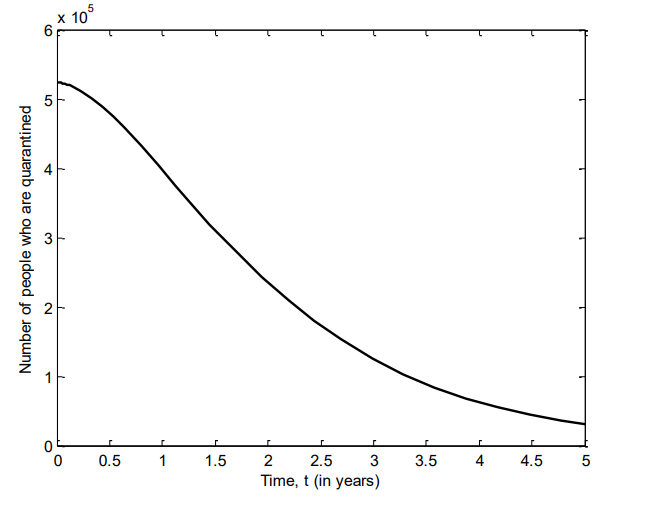
Figure 6 shows the number of individuals in Iraq who were in incubation stage of VZV between 2007 and 2011. Here, there is sharp increase of the number of individuals in incubation stage of the disease, and start to decline after two years.
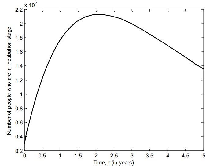
Figure 7 shows the number of individuals in Iraq who were in prodromal stage of VZV between 2007 and 2011. Here, there is sharp increase of the number of individuals prodromal stage of the disease, and continue to decline after three years.
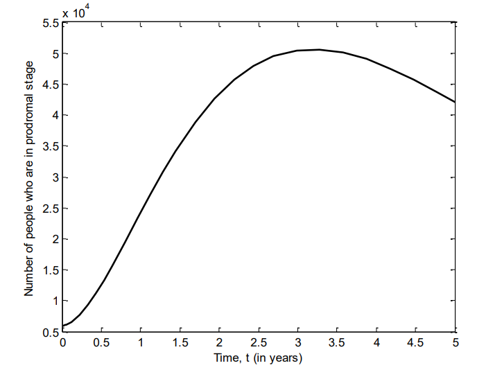
Figure 8 shows the number of individuals in Iraq who were in active stage of VZV between 2007 and 2011. It is observed that at the beginning, there is a reduction of individuals at this stage, but after about seven months, there is a spike leading to a sharp increase until the fourth year where it starts to decline.
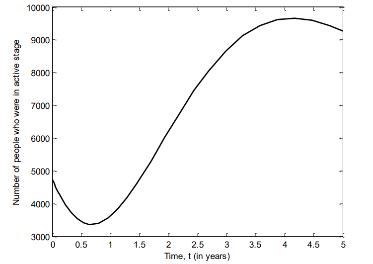
Figure 9 shows the number of individuals in Iraq who were hospitalized of VZV between 2007 and 2011. Here, there is sharp increase of the number of individuals into the hospital, and start to decline after two and a half years.
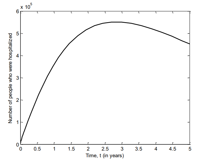
Figure 10 shows the number of individuals in Iraq that recovered from VZV between 2007 and 2011. It is observed that over time, individuals will continue to recover from the disease.
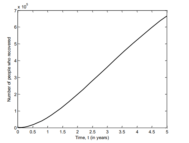
Figure 11 shows the number of individuals in Iraq who are in incubation stage of VZV between 2007 and 2025 for different values of \(\beta\).
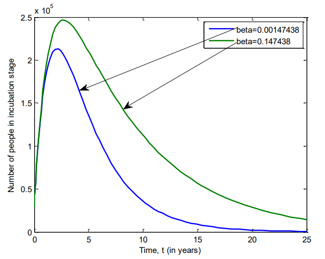
Figure 12 shows the number of individuals in Iraq who were in prodromal stage of VZV between 2007 and 2025 for \(\beta=0.00147438\) and \(\beta=0.147438\).
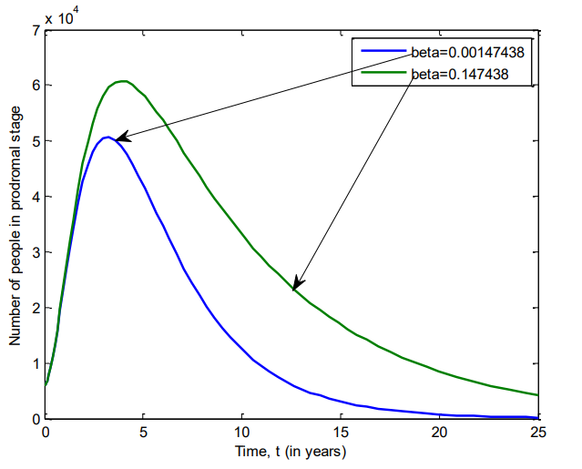
Figure 13 shows the number of individuals in Iraq who were in active stage of VZV between 2007 and 2025 for \(\beta=0.00147438\) and \(\beta=0.147438\).
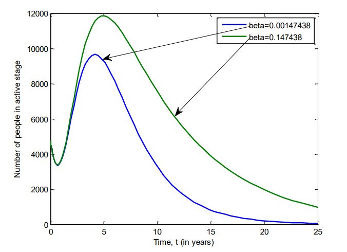
Figure 14 shows the number of individuals in Iraq who were hospitalized of VZV between 2007 and 2025 for \(\beta=0.00147438\) and \(\beta=0.147438\).
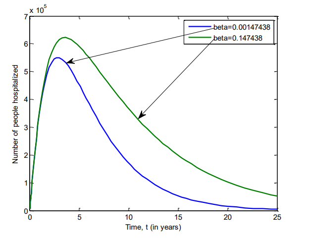
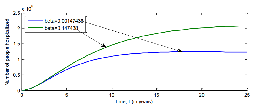
Figure 15 shows the number of individuals in Iraq recovered from VZV between 2007 and 2025 for \(\beta=0.00147438\) and \(\beta=0.147438\).
The mathematical modelling of chickenpox disease and stability analyses of our \(SEQI_1I_2I_3I_4R\) model are discussed in this paper. The proof of global stability of the local and global stable endemic equilibriums in a positive invariant subset of a given feasible region were successfully established. Also, the basic reproduction number of our model was obtained. Some simulation results are carried out in this paper, using Iraq as a case study. In which, we found that the exposed and quarantined classes declined in numbers. There was also sharp increase of the number of individuals in incubation stage of the disease, and start to decline after two years. Also, there was a sharp increase of the number of individuals prodromal stage of the disease, and continue to decline after three years. It was found also that at the beginning, there was a reduction of individuals at this stage, but after about seven months, there is a spike leading to a sharp increase until the fourth year where it starts to decline. Again, there was a sharp increase of the number of individuals into the hospital, and start to decline after two and a half years. It was found in this paper, that subdividing the infected class into subclasses to captured the true nature of chickenpox stages, will give the researchers and medical practitioneers an incite of the roles of chickenpox progression stages, as well as the contact rate will play in affecting and contributing to the spread of the disease in a population. Quarantine as a control strategies was found to be effective and efficient measure in the control of the spread of chickenpox in our population.