
The heat equation is a classical verification problem for numerical methods because it is analytically tractable while retaining the principal structure of parabolic diffusion. In many applications, however, the boundary is not a passive location at which only a value or flux is prescribed. Surface storage, kinetic exchange, membrane effects, and active interfacial dynamics may lead to boundary laws containing a time derivative of the unknown on the boundary. Such conditions are commonly described as Wentzell-type, generalized Wentzell, kinetic, or dynamic boundary conditions, depending on the analytical context and sign convention [1– 3].
Physics-informed neural networks (PINNs) approximate solutions of differential equations by embedding the governing equations and auxiliary constraints into a residual-minimization objective [4– 6]. Their appeal lies in the use of automatic differentiation or exact differentiated basis functions to evaluate differential operators at scattered collocation points, thereby allowing a mesh-free approximation strategy. PINNs and related physics-informed methods have been investigated for heat-transfer problems, diffusion models, inverse thermal problems, and phase-change models [7– 11]. At the same time, the literature has identified several recurrent difficulties, including loss imbalance, optimization pathologies, seed sensitivity, and deceptively small residuals that may coexist with poor physical fidelity [12– 14].
Dynamic boundary conditions are especially well suited for exposing these issues. A reliable solver must satisfy the interior heat equation and, simultaneously, endpoint evolution laws involving \(u_t\), \(u\), and a spatial derivative. This introduces several opportunities for benchmark misinterpretation. A manufactured solution may satisfy the dynamic boundary law while accidentally nullifying the boundary-gradient term. Likewise, a small interior residual does not imply that the dynamic boundary conditions are satisfied, and visual agreement in plots does not replace explicitly tabulated error and residual calculations.
This study addresses those concerns by constructing and documenting a small but fully specified benchmark suite. Two manufactured solutions are used: a reduced dynamic-boundary test that makes the compatibility condition for homogeneous forcing explicit, and a fully active Wentzell-gradient test that activates the \(\beta u_x\) contribution at both endpoints. The paper reports directly computed error and residual measures, an executed finite-difference baseline, five-seed variability, and an ablation study. The neural approximation adopted for the numerical tables is a least-squares physics-informed random-feature network, closely related to physics-informed extreme learning machines [15, 16]. This choice is deliberate. Because the benchmark problem is linear, fixing the hidden features and solving a regularized linear least-squares system yields a reproducible residual-minimizing neural approximation while avoiding ambiguity associated with optimizer settings, local minima, and learning-rate schedules. Standard fully trainable PINNs can also be applied to the same benchmark, but the results reported here are based only on the directly computed least-squares random-feature formulation.
Let \(Q=(0,1)\times(0,T]\). The interior equation is \[u_t(x,t)=\alpha u_{xx}(x,t), \qquad (x,t)\in Q, \label{eq:pde} \tag{1}\] with initial condition \[u(x,0)=u_0(x), \qquad x\in[0,1]. \label{eq:ic} \tag{2}\]
The dynamic boundary conditions are written as \[ u_t(0,t)+k u(0,t)+\beta u_x(0,t) =g_0(t), \label{eq:bc0}\ \tag{3}\] \[u_t(1,t)+k u(1,t)-\beta u_x(1,t) =g_1(t), \label{eq:bc1} \ \tag{4}\] for \(t\in(0,T]\), where \(\alpha>0\), \(k\ge 0\), and \(\beta\in\mathbb{R}\). The outward normal derivative is \(\partial_\nu u(0,t)=-u_x(0,t)\) and \(\partial_\nu u(1,t)=u_x(1,t)\). Hence (3)–(4) may also be written compactly as \[u_t+k u-\beta\partial_\nu u=g \quad \text{on } \partial(0,1), \tag{5}\] with endpoint-specific forcing values. The sign convention is stated explicitly because different formulations of Wentzell and dynamic boundary conditions appear in the literature.
All numerical experiments in this paper use \[\alpha=1, \qquad \beta=1, \qquad k=\pi^2, \qquad T=0.5. \label{eq:parameters} \tag{6}\]
Benchmark A is defined by \[u_A^\ast(x,t)=\mathrm{e}^{-\alpha\pi^2 t}\cos(\pi x). \label{eq:exactA} \tag{7}\]
It satisfies the interior equation because \((u_A^\ast)_{xx}=-\pi^2 u_A^\ast\). The initial condition is \(u_0(x)=\cos(\pi x)\). Substitution into the boundary laws gives
\[ g_{0,A}(t) =(k-\alpha\pi^2)\mathrm{e}^{-\alpha\pi^2 t},\label{eq:g0A}\ \tag{8}\] \[g_{1,A}(t) =(\alpha\pi^2-k)\mathrm{e}^{-\alpha\pi^2 t}.\label{eq:g1A} \ \tag{9}\]
Thus homogeneous forcing, \(g_{0,A}\equiv g_{1,A}\equiv 0\), is valid if and only if \[k=\alpha\pi^2. \label{eq:compat} \tag{10}\]
This compatibility condition is imposed in (6).
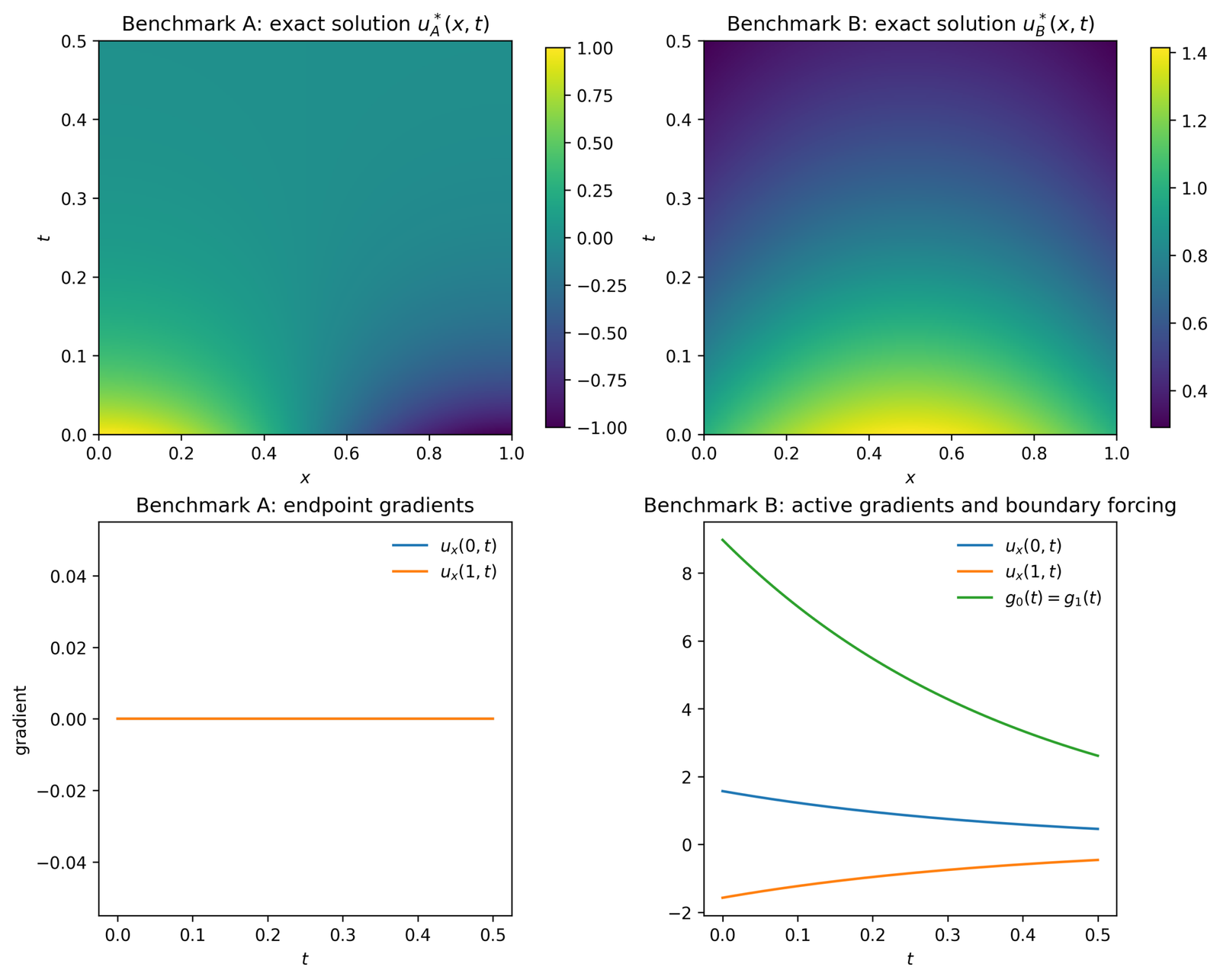
Benchmark A is intentionally retained even though it does not activate the boundary-gradient term. Since \[\partial_x u_A^\ast(x,t)=-\pi\mathrm{e}^{-\alpha\pi^2t}\sin(\pi x), \tag{11}\] we have \(\partial_xu_A^\ast(0,t)=\partial_xu_A^\ast(1,t)=0\). Consequently, the \(\beta u_x\) contribution in (3)–(4) is inactive. Benchmark A is therefore a reduced Wentzell test: it verifies the interior diffusion equation, the dynamic boundary time derivative, the boundary reaction term, and the compatibility condition for homogeneous forcing, but not the flux contribution itself.
Benchmark B is constructed to test the boundary-gradient contribution directly. It is defined by \[u_B^\ast(x,t)=\mathrm{e}^{-\alpha\omega^2t}\{\cos(\omega x)+\sin(\omega x)\}, \label{eq:exactB} \tag{12}\] with \(\omega>0\). The interior equation is again satisfied because \[\partial_{xx}\{\cos(\omega x)+\sin(\omega x)\}=-\omega^2\{\cos(\omega x)+\sin(\omega x)\}. \tag{13}\]
The forcing terms required by (3)–(4) are \[ g_{0,B}(t) =(k-\alpha\omega^2+\beta\omega)\mathrm{e}^{-\alpha\omega^2t},\label{eq:g0B}\ \tag{14}\] \[g_{1,B}(t) =\mathrm{e}^{-\alpha\omega^2t}\left[(k-\alpha\omega^2)(\cos\omega+\sin\omega)-\beta\omega(\cos\omega-\sin\omega)\right].\label{eq:g1B} \ \tag{15}\]
The endpoint derivatives are \[ \partial_xu_B^\ast(0,t) =\omega\mathrm{e}^{-\alpha\omega^2t},\label{eq:Bleftderiv}\ \tag{16}\] \[\partial_xu_B^\ast(1,t) =\omega\mathrm{e}^{-\alpha\omega^2t}(\cos\omega-\sin\omega).\label{eq:Brightderiv} \ \tag{17}\]
For the numerical study, \[\omega=\frac{\pi}{2}. \tag{18}\]
Then both endpoint derivatives are nonzero: \[\partial_xu_B^\ast(0,t)=\frac{\pi}{2}\mathrm{e}^{-\pi^2t/4}, \qquad \partial_xu_B^\ast(1,t)=-\frac{\pi}{2}\mathrm{e}^{-\pi^2t/4}. \tag{19}\]
With the parameter choice (6), the two forcing terms coincide, \[g_{0,B}(t)=g_{1,B}(t)=\left(\frac{3\pi^2}{4}+\frac{\pi}{2}\right)\mathrm{e}^{-\pi^2t/4}. \label{eq:forcingBsimplified} \tag{20}\]
Table 1 summarizes the two manufactured benchmarks. Benchmark A is a reduced compatibility and implementation test, whereas Benchmark B is a fully active Wentzell-gradient test. Figure 1 visualizes the two benchmark solutions and their endpoint behavior. The lower-left panel highlights the flux-term degeneracy of Benchmark A, while the lower-right panel shows that Benchmark B has nonzero endpoint derivatives and nonzero boundary forcing throughout the time interval.
| Quantity | Benchmark A | Benchmark B |
| Exact solution | \(e^-\pi^2t\cos(\pi x)\) | \(e^-\pi^2t/4\{\cos(\pi x/2)+\sin(\pi x/2)\}\) |
| Boundary forcing | \(g_0=g_1=0\) under \(k=\pi^2\) | \(g_0=g_1=(3\pi^2/4+\pi/2)e^-\pi^2t/4\) |
| Endpoint derivatives | \(u_x(0,t)=u_x(1,t)=0\) | \(u_x(0,t)=\pi e^-\pi^2t/4/2\), \(u_x(1,t)=-\pi e^-\pi^2t/4/2\) |
| Role of \(\beta u_x\) | Inactive | Active at both endpoints |
| Primary use | Compatibility and reduced dynamic-boundary verification | Fully active Wentzell-gradient verification |
The neural approximation used for the reported tables is \[u_\theta(x,t)=u_0(x)+t\sum_{m=1}^{M}c_m\phi_m(x,t), \label{eq:hardansatz} \tag{21}\] where \[\phi_m(x,t)=\tanh(a_m\widehat{x}+b_m\widehat{t}+d_m), \qquad \widehat{x}=2x-1, \qquad \widehat{t}=2t/T-1. \tag{22}\]
The factor \(t\) enforces \(u_\theta(x,0)=u_0(x)\) exactly. Consequently, the initial condition is not included as an active loss term in the hard-constrained runs. It is monitored separately through \[D_{\text{IC}}=\left(\frac{1}{N_{\text{IC}}}\sum_i |u_\theta(x_i,0)-u_0(x_i)|^2\right)^{1/2}, \tag{23}\] which is zero up to roundoff for (21).
The hidden-feature parameters \((a_m,b_m,d_m)\) are sampled independently for each seed, with \(a_m,b_m\sim\mathcal{N}(0,1.5^2)\) and \(d_m\sim\mathcal{U}[-1,1]\). Only the output coefficients \(c_m\) are solved. This random-feature formulation is more restrictive than a fully trainable deep PINN, but it is appropriate for a linear benchmark study because it produces a reproducible residual-minimizing approximation without the confounding influence of optimizer trajectories.
The interior residual is \[r_f(x,t)=\partial_tu_\theta(x,t)-\alpha\partial_{xx}u_\theta(x,t). \tag{24}\]
The endpoint residuals are \[ r_0(t) =\partial_tu_\theta(0,t)+ku_\theta(0,t)+\beta\partial_xu_\theta(0,t)-g_0(t),\label{eq:r0}\ \tag{25}\] \[r_1(t) =\partial_tu_\theta(1,t)+ku_\theta(1,t)-\beta\partial_xu_\theta(1,t)-g_1(t).\label{eq:r1} \ \tag{26}\]
Because (21) is linear in the unknown vector \( c=(c_1,\ldots,c_M)^T\), collocation of \(r_f\), \(r_0\), and \(r_1\) leads to a linear least-squares problem \[ c=\arg\min_{ z\in\mathbb{R}^M}\left\|A z- b\right\|_2^2+\lambda\| z\|_2^2, \label{eq:ridge} \tag{27}\] where \(\lambda=10^{-8}\) in all reported runs. The ridge term regularizes the normal equations while remaining small relative to the residual scales.
For each random-feature seed, the collocation set contains \(2000\) pseudorandom interior points and a \(44\times45\) tensor-product interior grid, giving \(N_f=3980\) interior collocation points. The boundary residuals are collocated at \(401\) equally spaced times per endpoint. Unless otherwise stated, \(M=250\) hidden features are used. All reported solution errors are computed on an independent \(301\times301\) evaluation grid. PDE residual RMS values are computed on \(12000\) evaluation points sampled from that grid, and boundary residual RMS values are computed on \(2001\) equally spaced boundary times.
For reproducibility, the differentiated basis terms are stated explicitly. Let \[z_m=a_m\widehat{x}+b_m\widehat{t}+d_m, \qquad s_m=1-\tanh^2(z_m). \tag{28}\]
For the hard feature \(\psi_m(x,t)=t\tanh(z_m)\) appearing in (21), \[ \partial_t\psi_m = \tanh(z_m)+t s_m b_m\frac{2}{T},\label{eq:psit}\ \tag{29}\] \[\partial_x\psi_m =2t a_m s_m,\label{eq:psix}\ \tag{30}\] \[\partial_{xx}\psi_m =-8t a_m^2 s_m\tanh(z_m).\label{eq:psixx} \ \tag{31}\]
Eqs. (29)–(31) are sufficient to assemble the least-squares matrix without automatic differentiation.
A deterministic classical solver is included to provide an independent baseline. Let \(x_i=ih\), \(i=0,\ldots,N\), with \(h=1/N\), and \(t^n=n\Delta t\). For interior nodes \(i=1,\ldots,N-1\), backward Euler gives \[\frac{u_i^{n+1}-u_i^n}{\Delta t} =\alpha\frac{u_{i+1}^{n+1}-2u_i^{n+1}+u_{i-1}^{n+1}}{h^2}. \label{eq:fdinterior} \tag{32}\]
The dynamic boundary laws are discretized as \[ \frac{u_0^{n+1}-u_0^n}{\Delta t}+ku_0^{n+1} +\beta\frac{-3u_0^{n+1}+4u_1^{n+1}-u_2^{n+1}}{2h} =g_0(t^{n+1}),\label{eq:fdleft}\ \tag{33}\] \[\frac{u_N^{n+1}-u_N^n}{\Delta t}+ku_N^{n+1} -\beta\frac{3u_N^{n+1}-4u_{N-1}^{n+1}+u_{N-2}^{n+1}}{2h} =g_1(t^{n+1}).\label{eq:fdright} \ \tag{34}\]
The one-sided spatial derivatives in (33)–(34) are second-order accurate. The time discretization is first-order, so the overall method is not second-order for an arbitrary time step. In the convergence study below, the parabolic scaling \(\Delta t=2h^2\) is used, making the first-order temporal error \(O(h^2)\) and allowing the spatial second-order behavior to be observed.
For a computed approximation \(u_h\), the reported relative errors are \[E_{L^2}=\frac{\|u_h-u^\ast\|_{L^2([0,1]\times[0,T])}}{\|u^\ast\|_{L^2([0,1]\times[0,T])}}, \qquad E_{L^\infty}=\frac{\|u_h-u^\ast\|_{L^\infty([0,1]\times[0,T])}}{\|u^\ast\|_{L^\infty([0,1]\times[0,T])}}. \tag{35}\]
The continuous norms are approximated by uniform-grid quadrature or evaluation on the stated grids. Residual magnitudes are reported as \[R_f=\left(\frac{1}{N_q}\sum_{i=1}^{N_q}|r_f(x_i,t_i)|^2\right)^{1/2}, \qquad R_j=\left(\frac{1}{N_b}\sum_{i=1}^{N_b}|r_j(t_i)|^2\right)^{1/2}, \quad j=0,1. \tag{36}\]
These metrics are reported explicitly to avoid the limitations of figure-only assessment.
Table 2 reports five-seed statistics for Benchmarks A and B. Benchmark A is solved with homogeneous boundary forcing under the compatibility condition \(k=\pi^2\). Benchmark B uses the fully active forcing (20). The statistics are computed over seeds \(s=0,1,2,3,4\).
| Benchmark | \(E_{L^2}\) | \(E_{L^{\infty}}\) | \(R_f\) | \(R_0\) | \(R_1\) |
|---|---|---|---|---|---|
| A | \((8.65\pm1.27)\times10^{-6}\) | \((1.12\pm0.20)\times10^{-5}\) | \((2.30\pm0.39)\times10^{-4}\) | \((1.94\pm0.84)\times10^{-4}\) | \((1.80\pm0.49)\times10^{-4}\) |
| B | \((9.45\pm2.42)\times10^{-8}\) | \((2.77\pm0.99)\times10^{-7}\) | \((9.87\pm2.77)\times10^{-6}\) | \((7.41\pm4.06)\times10^{-6}\) | \((8.15\pm2.00)\times10^{-6}\) |
The principal numerical observation is that Benchmark B is not only specified analytically but also solved and evaluated quantitatively. Its relative errors remain below \(10^{-6}\), while the RMS boundary residuals remain below \(10^{-5}\). Because \(u_x(0,t)\) and \(u_x(1,t)\) are nonzero in Benchmark B, these residuals test the active \(\beta u_x\) contribution in (3)–(4). Benchmark A produces larger errors and residuals than Benchmark B in the present implementation, primarily because the faster decay \(\mathrm{e}^{-\pi^2t}\) is more demanding for the fixed random-feature set than the milder decay \(\mathrm{e}^{-\pi^2t/4}\) in Benchmark B. Nevertheless, both cases display small relative errors and stable seed-to-seed behavior.
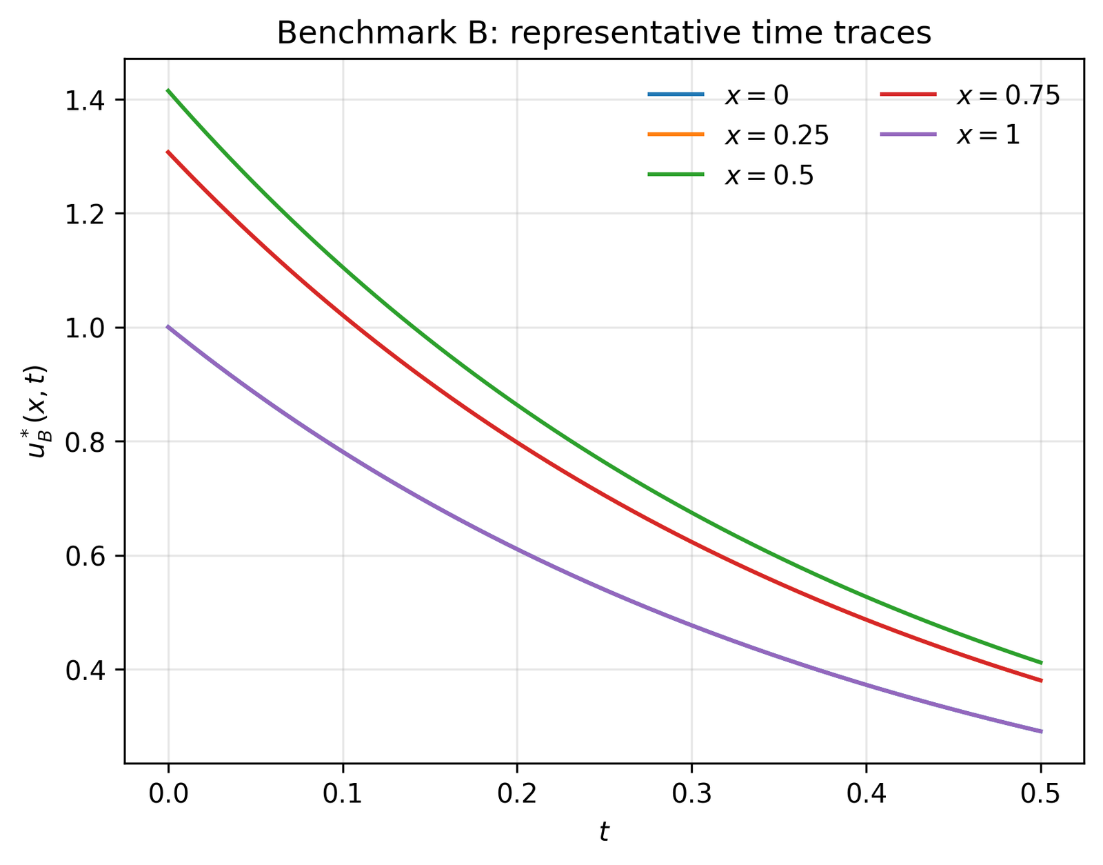
Figure 2 shows representative exact time traces for Benchmark B at several spatial locations. The figure highlights the smooth temporal decay and the variation in amplitude across the interval, which together make Benchmark B a useful complementary test to the flux-inactive cosine benchmark.
The individual seed values are listed in Appendix A, so the means in Table 2 do not obscure seed-to-seed variability.
Table 3 reports the finite-difference baseline. The observed convergence rate is computed from successive \(E_{L^2}\) values under grid refinement. Both benchmarks show rates close to two, as expected when second-order spatial differences are combined with the parabolic scaling \(\Delta t=2h^2\).
| Benchmark | \(N\) | \(\Delta t\) | \(E_{L^2}\) | \(E_{L^\infty}\) | observed order in \(E_{L^2}\) |
|---|---|---|---|---|---|
| A | 40 | \(1.2500\times10^{-3}\) | \(4.3439\times10^{-3}\) | \(2.2374\times10^{-3}\) | – |
| 80 | \(3.1250\times10^{-4}\) | \(1.0911\times10^{-3}\) | \(5.5944\times10^{-4}\) | 1.99 | |
| 160 | \(7.8125\times10^{-5}\) | \(2.7294\times10^{-4}\) | \(1.3974\times10^{-4}\) | 2.00 | |
| B | 40 | \(1.2500\times10^{-3}\) | \(3.8424\times10^{-4}\) | \(3.6238\times10^{-4}\) | – |
| 80 | \(3.1250\times10^{-4}\) | \(9.6462\times10^{-5}\) | \(9.0692\times10^{-5}\) | 1.99 | |
| 160 | \(7.8125\times10^{-5}\) | \(2.4151\times10^{-5}\) | \(2.2672\times10^{-5}\) | 2.00 |
The finite-difference results serve two purposes. First, they confirm that the manufactured solutions and forcing expressions are consistent with an independent discretization. Second, they show that the benchmark is not intrinsically difficult for a classical one-dimensional solver. The neural results should therefore be interpreted as verification of a physics-informed approximation strategy, not as evidence that the neural method is preferable to finite differences for this linear benchmark. Finite-difference convergence under the scaling \(\Delta t=2h^2\) is shown in Figure 3. Both manufactured benchmarks exhibit approximately second-order decay of the relative \(L^2\) error with respect to \(h\).
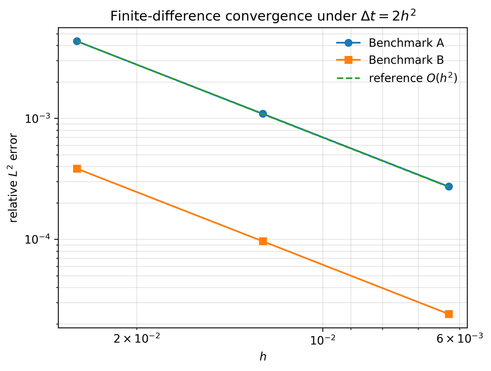
Table 4 reports a targeted ablation study on Benchmark B using seed \(0\). The most informative comparison is the removal of the boundary residual. When the least-squares system includes only the interior PDE residual while retaining the hard initial condition, the PDE residual remains small but the boundary residuals become \(O(1)\) and the relative \(L^2\) error increases to \(6.28\times10^{-2}\). This directly demonstrates why dynamic boundary residuals must be reported separately. A method can satisfy the interior equation quite well and still fail the Wentzell-type boundary law.
| Variant | \(E_{L^2}\) | \(E_{L^\infty}\) | \(R_f\) | \(R_0\) | \(R_1\) |
|---|---|---|---|---|---|
| Full setting | \(5.61\times10^{-8}\) | \(1.41\times10^{-7}\) | \(6.49\times10^{-6}\) | \(4.46\times10^{-6}\) | \(4.76\times10^{-6}\) |
| No boundary residual | \(6.28\times10^{-2}\) | \(1.75\times10^{-1}\) | \(4.50\times10^{-6}\) | \(4.16\times10^{-1}\) | \(1.37\) |
| Raw inputs, no scaling | \(9.96\times10^{-8}\) | \(1.35\times10^{-7}\) | \(4.53\times10^{-6}\) | \(4.00\times10^{-6}\) | \(4.29\times10^{-6}\) |
| Soft initial condition | \(1.67\times10^{-6}\) | \(5.59\times10^{-6}\) | \(7.61\times10^{-6}\) | \(2.83\times10^{-6}\) | \(2.74\times10^{-6}\) |
| \(M=100\) features | \(7.12\times10^{-5}\) | \(1.29\times10^{-4}\) | \(3.09\times10^{-3}\) | \(2.92\times10^{-3}\) | \(3.23\times10^{-3}\) |
| \(M=50\) features | \(2.48\times10^{-3}\) | \(4.86\times10^{-3}\) | \(4.31\times10^{-2}\) | \(4.51\times10^{-2}\) | \(6.11\times10^{-2}\) |
The scaling ablation is also informative. On this simple one-dimensional domain, replacing the scaled inputs with raw \((x,t)\) coordinates does not degrade the result and is slightly better for seed \(0\). Input scaling is therefore not claimed to be essential for this particular problem. The soft-initial-condition variant also performs well, with relative errors on the order of \(10^{−6}\), but its initial mismatch is no longer identically zero because the initial condition is enforced as a least-squares penalty rather than imposed exactly. Reducing the feature count has a clear effect: \(M=100\) remains accurate, whereas \(M=50\) is visibly under-resolved in both residual and solution-error metrics.
The numerical study supports four main conclusions. First, the benchmark suite benefits from a clear separation between a reduced dynamic-boundary test and a fully active Wentzell-gradient test. Benchmark A remains useful because it exposes the compatibility condition for homogeneous forcing and verifies the dynamic boundary time derivative and reaction terms. However, its endpoint derivatives vanish, so it cannot probe the boundary-gradient contribution. Benchmark B removes that degeneracy and therefore provides the more decisive verification case for the Wentzell-type term.
Second, the evidence is quantitative rather than purely visual. The principal claims are supported by relative \(L^2\) and \(L^\infty\) errors, RMS PDE residuals, and RMS boundary residuals, all computed on independent evaluation sets. The appendix gives per-seed values, so the reported mean values are traceable.
Third, the finite-difference baseline clarifies the nature of the contribution. A standard implicit finite-difference method solves the one-dimensional linear problem accurately and with predictable convergence. The contribution of the present paper is therefore not algorithmic dominance over classical solvers; rather, it is the provision of a transparent verification problem and a documented neural approximation workflow for dynamic boundary conditions.
Fourth, the ablation study shows why boundary-specific reporting is indispensable. The no-boundary-residual variant achieves a small interior PDE residual while simultaneously producing large boundary residuals and a much larger solution error. For dynamic boundary conditions, endpoint residuals should be reported individually rather than merged into a single opaque loss number.
Several limitations should also be stated clearly. The problem is linear, one-dimensional, smooth, and manufactured. The random-feature PINN used here is intentionally simpler and more reproducible than a fully trainable deep network; accordingly, the results do not imply that Adam–LBFGS PINNs, adaptive loss-balancing PINNs, or residual-adaptive PINNs will behave identically on the same benchmark. The finite-difference study is intended as a consistency check rather than a full computational-cost comparison. No claim is made about nonlinear Wentzell problems, higher-dimensional domains, irregular geometries, noisy data, or inverse parameter estimation.
This paper has presented a reproducible benchmark study of a physics-informed neural approximation for the heat equation with Wentzell-type dynamic boundary conditions. Two manufactured solutions were used: Benchmark A as a reduced compatibility test and Benchmark B as a fully active Wentzell-gradient test. The reported least-squares random-feature PINN solved both cases with small directly measured errors and residuals, while the finite-difference solver independently confirmed the correctness of the manufactured solutions and forcing terms.
The main contribution is a verification-oriented benchmark framework rather than a claim of general neural-solver superiority. Within the smooth one-dimensional setting studied here, the benchmark suite provides a transparent test bed for evaluating whether a neural method satisfies both the interior diffusion equation and the dynamic endpoint laws. This makes the benchmark suitable as a compact reference problem for future studies of PINNs and related methods under dynamic or Wentzell-type boundary conditions.
Table 5 gives the individual seed values underlying Table 2.
| Benchmark | Seed | \(E_{L^2}\) | \(E_{L^{\infty}}\) | \(R_f\) | \(R_0\) | \(R_1\) |
|---|---|---|---|---|---|---|
| A | 0 | \(7.8779\times10^{-6}\) | \(9.1372\times10^{-6}\) | \(1.7664\times10^{-4}\) | \(1.8964\times10^{-4}\) | \(1.6546\times10^{-4}\) |
| A | 1 | \(9.1684\times10^{-6}\) | \(1.3170\times10^{-5}\) | \(2.7907\times10^{-4}\) | \(2.0399\times10^{-4}\) | \(1.8062\times10^{-4}\) |
| A | 2 | \(8.4795\times10^{-6}\) | \(1.2272\times10^{-5}\) | \(2.0810\times10^{-4}\) | \(6.3552\times10^{-5}\) | \(1.6208\times10^{-4}\) |
| A | 3 | \(7.2177\times10^{-6}\) | \(8.9865\times10^{-6}\) | \(2.4523\times10^{-4}\) | \(2.9908\times10^{-4}\) | \(1.3225\times10^{-4}\) |
| A | 4 | \(1.0520\times10^{-5}\) | \(1.2235\times10^{-5}\) | \(2.4242\times10^{-4}\) | \(2.1243\times10^{-4}\) | \(2.6127\times10^{-4}\) |
| B | 0 | \(5.6107\times10^{-8}\) | \(1.4103\times10^{-7}\) | \(6.4871\times10^{-6}\) | \(4.4643\times10^{-6}\) | \(4.7574\times10^{-6}\) |
| B | 1 | \(9.8526\times10^{-8}\) | \(2.3459\times10^{-7}\) | \(8.9956\times10^{-6}\) | \(7.8165\times10^{-6}\) | \(9.9158\times10^{-6}\) |
| B | 2 | \(8.9069\times10^{-8}\) | \(2.6842\times10^{-7}\) | \(8.4953\times10^{-6}\) | \(4.3671\times10^{-6}\) | \(8.1352\times10^{-6}\) |
| B | 3 | \(1.1844\times10^{-7}\) | \(3.9317\times10^{-7}\) | \(1.2041\times10^{-5}\) | \(1.4208\times10^{-5}\) | \(9.0877\times10^{-6}\) |
| B | 4 | \(1.1037\times10^{-7}\) | \(3.4885\times10^{-7}\) | \(1.3329\times10^{-5}\) | \(6.1750\times10^{-6}\) | \(8.8428\times10^{-6}\) |
For each interior point \((x_i,t_i)\), the corresponding row of the least-squares matrix is \[A^{(f)}_{im}=\partial_t\psi_m(x_i,t_i)-\alpha\partial_{xx}\psi_m(x_i,t_i), \tag{37}\] and the right-hand side is \[b^{(f)}_i=\alpha u_0''(x_i), \tag{38}\] because the base function \(u_0(x)\) contributes \(-\alpha u_0''(x)\) to the PDE residual. For the left endpoint, \[A^{(0)}_{im}=\partial_t\psi_m(0,t_i)+k\psi_m(0,t_i)+\beta\partial_x\psi_m(0,t_i), \tag{39}\] with \[b^{(0)}_i=g_0(t_i)-ku_0(0)-\beta u_0'(0). \tag{40}\]
For the right endpoint, \[A^{(1)}_{im}=\partial_t\psi_m(1,t_i)+k\psi_m(1,t_i)-\beta\partial_x\psi_m(1,t_i), \tag{41}\] with \[b^{(1)}_i=g_1(t_i)-ku_0(1)+\beta u_0'(1). \tag{42}\]
Stacking these rows yields (27). This formulation is included so that the reported tables can be regenerated without relying on automatic differentiation.
The reported neural calculations use double-precision NumPy linear algebra. For each seed \(s\in\{0,1,2,3,4\}\), the pseudorandom generator is initialized with that seed before drawing the random-feature weights, random-feature biases, and pseudorandom interior collocation points. The deterministic tensor-product interior points, boundary times, and evaluation grids are identical for all seeds. The finite-difference matrix is constant in time and is factorized once for each grid size. No external dataset is used.
The numerical values in the tables were generated using the following fixed settings: \(M=250\), random-feature scale \(1.5\), ridge parameter \(10^{-8}\), \(N_f=3980\) interior collocation points, \(401\) boundary times per endpoint, a \(301\times301\) solution evaluation grid, \(12000\) sampled PDE-residual evaluation points, and \(2001\) boundary-residual evaluation times. For the finite-difference study, \(N\in\{40,80,160\}\) and \(\Delta t=2h^2\) adjusted to reach \(T=0.5\) exactly.
The source package accompanying this manuscript contains the cleaned Python implementation used to assemble the least-squares system, compute the finite-difference baseline, evaluate the reported metrics, and generate the figures. This organization is intended to make independent verification straightforward.