Quaternionic Rank-Three Readout and Dual-Time Reconstruction: Inner Generation, Outer Dynamics, and Phase Actions

1. Introduction: Reconstruction Before Primitive Insertion

1.1. The Carrier Problem

The mathematical foundations of physics commonly begin with several highly successful structures already in place: a complex Hilbert space, an imaginary unit acting on amplitudes, a three-dimensional displacement space, a record structure for observation, and a Lorentzian geometry for causal readout. The present paper asks a question about the logical dependencies preceding these choices. Which of these roles can be reconstructed from more elementary recurrence, completion, representation, and covariance data, and which must remain explicit inputs?

This question will be called the carrier problem. A carrier is the mathematical object on which a role can be expressed: a real plane can carry circular phase, a quaternion algebra can carry order-sensitive composition, a quotient module can carry displacement, and a complex line bundle can carry phase transport. Standard constructions show how such carriers behave once given. A reconstruction program instead asks why a stated class of source, completion, and record constraints selects one carrier rather than another.

Historically, the motivating program was developed under the names Single Monad Model and Duality of Time Theory. Here their dual-time distinction is given a finite mathematical meaning: inner generative time orders the acquisition of independent tests, an outer completion event makes a record available, and outer completion time orders those events. Dynamics on that outer order is induced only when the completed records retain the information needed for prediction. This use of two temporal roles is distinct from assuming two timelike spacetime coordinates. The theorem statements use these roles explicitly, so they can be evaluated independently of the broader interpretation. The formal results depend on the displayed source, algebra, representation, record, and reconstruction data, not on acceptance of a separate metaphysical thesis.

1.2. Generative Histories, Completed Records, and Quotient Selection

The broader reconstruction architecture distinguishes a level at which admissible histories compose from a level at which observers access completed records. A minimal schematic is

Here \(X\) is a generative state space, \(\mathsf{Hist}\) is a monoid or category of admissible histories, \(\kappa\) is a completion or stabilization map, and \(\pi\) is an observational projection. Completion and projection are not synonyms: completion determines when a stable record exists, whereas projection determines which information in that completed record is accessible to a specified observational protocol.

This separation turns the otherwise vague phrase “projection of reality” into a selection problem. Given a class \(\mathsf{Hist}_{\mathrm c}\) of admissible completed-future continuations and a family \(\mathcal O\) of observer-level tests, define the deterministic behavioral equivalence

The quotient \(X/{\equiv_{\mathcal O}}\) is the coarsest deterministic presentation preserving all declared completed-future tests. In a stochastic realization, equality of test values is replaced by equality of the full laws of future completed tests; the resulting predictive quotient is the minimal sufficient observable state for that test family. Choosing the test family is itself a physical selection problem. A natural variational target is to minimize retained complexity or redundancy subject to preserving the relevant future laws and stable records.

The finite linear criterion in Proposition 1 makes the future-preserving quotient precise for a supplied cycle map; Proposition 4 gives its quantum counterpart through invariance of the accessible observable algebra. The word protocol of Theorem 4 then generates a complete family of center-insensitive tests and its rank-three readout. Separately, the reconstruction theorem distinguishes a pre-closure graded object from a linearized output diagram. The latter is obtained through a precisely defined functor that forgets algebraic structure and totalizes graded spaces; it is not asserted to be the physical completion map \(\kappa\), the observation map \(\pi\), or their composite.

1.3. The Focused Mathematical Problem

Within that broader architecture, this paper isolates one carrier-and-reconstruction branch:

Given an explicitly selected phase field, quaternionic extension, and covariant functional space, what free reconstruction follows from symmetric pairing, alternating branching, and homogeneous propagation; how does it change under relations, flag transport, and a change of phase action?

The answer is conditional but exact. The object-level chain is

The reconstruction carries two inequivalent circle actions. The polynomial action inherited from the pre-closure grading satisfies

whereas a separately stated common-output rule gives the coherent character below; after an oriented output–Hopf identification \(\Phi_{\mathrm{out,H}}\), its associated determinant line satisfies

A further determinant-neutral closure principle selects the finite subgroup \(\boldsymbol\mu_{137}^{\mathrm{out}}\) and its least positive transported phase \(1/137\). The dimension is specific to the declared signature; the determinant kernel of a common weight-one \(n\)-dimensional output is, in general, \(\mu_n\). The rank-defect and flag-stabilizer results below identify structural information that this integer alone does not contain. The full and relative vacuum templates of Definition 16 have exact indices \(137\) and \(128\) before holonomy- and mass-dependent dressing. Their identification with inverse couplings requires the separate response-normalization problem of §12.5.

1.4. Inner Generation, Outer Completion, and Physical Realization

The SMM/DTT distinction is implemented by three separate operations: ordered inner acquisition generates tests, completion fixes which records are identified, and outer transport compares successive completed records. Theorem 4 and Corollary 3 establish finite generation and stability. Theorem 19 then applies outer autonomy to the relative vacuum sector: a hidden depth-two relation is consistently discarded only when it cannot reappear in future records. The criterion is imposed on a completed cycle, not necessarily on each inner step.

The conditional uniqueness statement in Theorem 18 joins the two parts of the construction: inner words generate the flag dimensions \(1,2,3\), and the declared free-completion laws determine the quadratic and exterior receivers on that flag. In particular, ten is the dimension of the full symmetric-square carrier, not a chosen numeral base. The ordered rank pair \((137,128)\) is fixed within those laws and the stated relative comparison; dimension three alone does not select the laws.

The resulting indices \(137\) and \(128\) are attached to completion sectors. Probe energy, outer duration, and spectral dressing are distinct variables. Theorem 25 states exactly which normalization assumptions turn the indices into reference responses, while Proposition 30 computes one finite holonomy–gap dressing mechanism. The physical question is whether one independently selected inner dynamics supplies the receiver, completion, mass ratios, transport, and absolute electromagnetic response. The conditional constructions make that question calculable without assuming its answer.

1.5. Quantum-Kinematic and Formation Interface

The phase-selected real Hilbert sector admits complex unitary kinematics, and the quaternionic spinor supplies projective rays and the \(SU(2)\to SO(3)\) cover. In the algebraic readout theorem, a record is a real functional, and observation consists of evaluating that functional; in the operational quantum template a record is a selected instrument outcome with a trace probability rule. The distinction is explicit. §3.3 supplies a normalized instrument and a criterion for autonomous reduced dynamics, while Proposition 8 identifies the readout geometry with the Bloch ball under a stated state interpretation. Proposition 9, Theorem 6, and Corollary 4 give an explicit operational realization: the word-generated tests determine a qubit state, and a time-independent recorder exposes the joint statistical cost of phase overlap and incomplete execution. These results assume quantum preparations and the trace probability rule; they do not derive that rule from a dimension count.

For spacetime, the completed cone determines local Lorentzian conformal geometry. A smooth coframe and spin realization then connect the same spatial carrier to Dirac and Maxwell propagation in §12.2. For electromagnetic coupling, the unresolved scalar is the normalized kinetic response, for which Sections 12.4, 12.5, and 12.6 give reduction, normalization, and spectral-response results. Proposition 31 and Proposition 32 add a sharp response bound and a specified local quadratic matching. The finite receiver remains distinct from a field Fock space, and global spacetime gluing, physical state preparation, and continuum dynamics remain realization tasks. Table 1 records these dependencies.

Table 1. Single claim-status ledger: supplied data, mathematical consequences, and missing realization maps.

Supplied data or rule	Proved consequence	Additional physical input
Alternating phase words and rank completion	Three tests generated successively; commutator span \(W\); stable recovery; kernel \(\mathbb{R}1\).	Selection of protocol and its physical implementation.
Cycle map and completed readout; specified quantum apparatus	Kernel/algebra criteria for autonomy; explicit word instrument, finite recorder and all-attempt error.	Trace rule, ready states, loaded dilation, couplings, clock calibration and reset.
Real flow and oriented phase maps	Positive-frequency phase on the dynamic sector; phase maps relate distinct carriers.	A physically selected flow and observable algebra.
Positive norm, associativity, incompatible phases	Quaternionic carrier and spinor/Hopf geometry.	A mechanism realizing the extension and its operations.
Nonzero center-insensitive invariant functional space	Rank-three instantaneous quotient; future tests can require more information.	Histories, completion, tests, and displacement correspondence.
Completed histories, sharp cone; smooth coframe and local action when supplied	Lorentzian cone; compatible Dirac–Maxwell characteristics; \(\alpha_{\mathrm{eff}}=q_m^2/(4\pi Z)\).	Continuum realization, field dynamics, quantization, and independent kinetic response.
Unital envelope, free symmetric and alternating laws, flag, homogeneous adjoining	Initial receiver of dimension \(137\); rank-defect comparison; obstruction to extending its flag-stabilizer action to \(SO(3)\).	Selection of this signature, faithful retention, and treatment of flag data.
Height-two comparison, selected embedding and phase action	Rank-\(128\) quotient; terminal defect nine; coherent weight \(128\), polynomial weight \(590\).	Selection of null records and dynamics; Theorem 19 tests autonomy; rank alone does not fix response.
Forgetting branch multiplication; optionally totalizing	Linear diagram retains the transported polynomial action with determinant \(z^{612}\).	A completion/observation realization of the forgetting operation.
Normalized coherent-output rule	Unique scalar-diagonal compatible action in its declared class; determinant \(z^{137}\) on the free receiver.	Independent reason to choose this action.
Oriented \(\Phi_{\mathrm{out,H}}\); additional determinant-neutrality criterion	Hopf determinant \(\mathcal L_{\mathrm H}^{\otimes137}\); if the criterion is adopted, closure subgroup \(\boldsymbol\mu_{137}^{\mathrm{out}}\).	Physical comparison cycle, matter line, connection, and action normalization.

1.6. Focused Contribution and Useful Consequences

The classical ingredients are used explicitly: finite representations, polar decomposition, Frobenius rigidity, symmetric and exterior universal properties, Hopf bundles, quantum channels, Clifford symbols, and Gaussian elimination. The initiality proof is an application of the direct-sum universal property, and Theorem 14 establishes uniqueness only inside a fixed signature. We do not claim a new general theory of free objects or polynomial functors.

The contribution is the analysis of this particular reconstruction and the extent to which information can be discarded while preserving its specified structure:

1. (N1) Proposition 1, Theorem 4, and Proposition 6 give a finite dual-time foundation: stable, order-sensitive generation of three tests, a criterion for autonomous completed-record dynamics, and a compatible outer flow. The quantum criterion in Proposition 4 adds exact subsystem autonomy; Proposition 9, Theorem 6, and Corollary 4 add an instrument, an autonomous completion certificate, and its exact all-attempt risk. With calibrated sharp propagation, Theorem 24 and Proposition 27 connect the readout to a Lorentzian cone and compatible field characteristics; Proposition 28 supplies a conditional kinetic-response calculation.

2. (N2) Theorem 17, Corollary 8, and Theorem 19 turn \(137-9=128\) into an exact sequence and a completion sector, locate its relations at the terminal stage, and characterize autonomous outer transport and holonomy descent. Theorem 18 states the conditional uniqueness of both ranks from the generated flag and declared laws. Alternative embeddings expose the remaining selection problem; Proposition 22 quantifies approximate autonomy over repeated cycles.

3. (N3) Theorem 15 compares every generated linear receiver with the free one and quantifies the loss caused by relations. Dimension \(137\) is attained exactly when all three adjoining maps are injective.

4. (N4) Theorem 16 computes the complete flag-stabilizer character of the output and proves that it does not extend to an \(SO(3)\) representation on the same fiber. Flag-independent dimension therefore does not entail a flag-independent rotational receiver. Theorem 20 sharpens this obstruction into attained maximal quotient dimensions \(133\) and \(127\), depending on the retained phase action.

5. (N5) Proposition 17, Proposition 23, and Proposition 24 distinguish the multiplication obstruction from construction grading, and separate the transported polynomial action from the additionally chosen coherent action.

6. (N6) Proposition 29, Theorem 25, and Proposition 30 separate exact vacuum indices, absolute response normalization, and spectral dressing. The finite model computes the corrections and their signs without claiming an electromagnetic prediction. Proposition 31 and Proposition 32 constrain the allowed dressing and calculate a local quadratic coefficient under a specified plaquette realization.

These consequences provide tests for later realizations: additional relations change the retained rank and coherent determinant, and removing the flag requires more than a choice of basis. The worked model in §10.1 verifies simultaneous compatibility of the input layers. A focused comparison with universal-construction and polynomial-functor literature appears in §13.2.

1.7. Conceptual and Mathematical Provenance

The historical vocabulary of a single generative source, recurrent re-creation, and two temporal roles appears in the author’s monographs [1,2]. Published developments include dual-time geometry and observable-time reductions [3], and real-commutant classification with positive-frequency phase selection [4,5]; related real-Hilbert reconstruction results appear in [6]. These references provide context and attribution. The constructions used here, including phase selection, quaternionic readout, the \(137\)–\(128\) comparison, quantum autonomy, completion-compatible holonomy, and the conditional cone and response results, are stated and proved from displayed hypotheses using standard mathematical inputs. The finite completion-event formalism is not claimed to be equivalent to every coordinate realization of dual time in the cited work.

1.8. Claim Status

A constitutive rule selects the class of models; a theorem gives consequences inside that class; a realization hypothesis connects the resulting mathematics to a specified physical procedure. The word schedule, rank-completion rule, supplied outer generator, unital envelope, symmetric and alternating free laws, homogeneous recursion, coherent-output action, and determinant-neutral closure criterion belong to the first category. Their consequences, including the comparison and obstruction results, belong to the second. The calibrated-history bounds and isotropic sharpness likewise define a conditional kinematic model. Physical spatial formation, its clock and cone realization, particle persistence, and electromagnetic matching remain in the third. The term vacuum template denotes the undressed reference in Definition 16; a physical vacuum state and the unit-response normalization in Theorem 25 are additional realization data. A proved conditional result is not an empirical establishment of SMM/DTT.

1.9. Development-History and Model-Selection Disclosure

The integers \(137\) and \(128\), including their familiar numerical proximity to inverse electromagnetic couplings in different settings, were known before these constructions were formulated. The displayed functors, maps, alternatives, and obstruction results establish logical dependence and reproducibility, not historically blind discovery. A physical comparison must follow a fixed choice of admissible functors, phase action, closure test, line conventions, regulator, and response law. The vacuum-sector interpretation concerns what the exact integers label; it does not turn their historical selection into a blind numerical prediction. The explicit field and response templates below do not change that requirement.

2. Foundational Principles of Generative and Observable Reconstruction

The historical program supplies motivation, but the principles below are written in role-based form. They are not all theorem hypotheses. Some specify explanatory direction; some define the class of reconstructions to be studied; and some identify open selection problems. Their purpose is to prevent formation, completion, observation, phase, and geometric readout from being collapsed into one undefined process.

Principle 1 (Reconstruction before primitive insertion). Complex phase, observable irreversibility, spatial readout, and causal geometry should be reconstructed from explicit input layers whenever possible, rather than introduced as unrelated primitives. When a structure cannot yet be reconstructed, it must remain a named datum or matching target.

Principle 2 (Generative–observable separation). Admissible histories compose at a generative level, while observation accesses completed records. The generative order need not be exposed by the observable record order. This is a functional separation between formation and completed comparison, not the postulation of two coordinate-time dimensions in spacetime.

Principle 3 (Completion). A generative history becomes observationally available only after a completion operation. Depending on the realization, completion may mean closure, stabilization, redundancy formation, environmental selection, reflective closure, sheafification, or another procedure that produces an identifiable record. Completion is conceptually distinct from the later loss of information under projection.

Principle 4 (Projection realism). Projection maps a completed state to the information accessible to a declared protocol and may identify distinct completed or generative histories. The resulting structures are nevertheless empirically real when they are stable under admissible perturbation, repeatably accessible, intersubjectively recordable, and integrated into successful explanation. Thus projection expresses a level of grounding, not a contrast between reality and illusion.

Principle 5 (Behavioral and predictive quotient selection). Projection is not treated as an arbitrary many-to-one map. Once a completion rule, a class of completed-future continuations, and a test family are fixed, the observable quotient is required to be the coarsest quotient preserving those tests. In stochastic models, observable states should form a minimal sufficient statistic for the laws of future completed tests.

Principle 6 (Stable records and minimal predictive presentation). Observable physics is formulated on record sectors that remain identifiable under the continuation, completion, and comparison operations of the protocol. Among prediction-preserving descriptions, the selected presentation should retain no unnecessary complexity or redundancy. This is a selection target, not a theorem proved in the present finite reconstruction.

Principle 7 (Generative monism and source–carrier–record separation). Empirical multiplicity is grounded in one functional generative source \(\mathsf{G}\), historically called the Monad. The source is not a localized particle, field, observer, hidden classical object, or constituent inside spacetime. Nontrivial mathematics is carried instead by admissible histories, real and complex carriers, completion operations, and record quotients. The same source may therefore underlie many derivative structures without those structures being unreal.

Principle 8 (Re-creation). At a record label \(t_{\mathrm r}\), a realized configuration may be modeled as the closure or readout of an inner recurrent pattern. Persistence is stability of the recurrence-and-closure class across successive records; motion is record-level continuity grounded in ordered renewal, rather than the primitive traversal of a permanently constituted object through an already completed continuum.

A continuous recurrence template, distinct from the finite word protocol constructed below, is

where the first relation expresses inner monodromy and the second denotes an outward record or closure map. The finite construction below specifies an ordered test-generation protocol and algebraic completion, while this continuous monodromy law, a physical \(\mathcal P_{\mathrm{out}}\), and a microscopic re-creation period remain realization data.

Principle 9 (Boundary closure). An observed event is an outer boundary closure of an inner recurrence pattern. A boundary may select closed modes, suppress or transmit amplitudes, or separate alternatives into distinguishable records. This is an interpretation of the conservative amplitude calculus, not a new stochastic collapse law or a derivation of the Born rule.

Quantum Record Interface.

The finite quantum realization in §3.3 composes unitary inner operations before recording an instrument outcome. The resulting outer channel is positive and normalized, while exact autonomy from arbitrary correlated states requires an invariant accessible observable algebra. This supplies a conservative record model under the usual trace probability rule. Selecting the record interaction and explaining its physical stability remain separate tasks.

Principle 10 (Phase/readout separation). Compact recurrence, complex phase, completed-record order, and Lorentzian causal readout are different structural roles. Compact sectors support phase; hyperbolic sectors support causal split geometry. They may be related in a larger architecture but must not be identified merely because each is described using the word “time.”

Principle 11 (Primitive projective-source interpretation). The generative source is not identified with a localized magnetic monopole. The controlled geometric interpretation is that the first nontrivial projective phase line downstream of the source may carry the primitive integral class \(\left\lvert c_1\right\rvert=1\). Any identification with a physical magnetic monopole, photon-polarization line, or electromagnetic charge unit requires a separate bundle-and-connection realization.

Principle 12 (Conservative compatibility and constraint-relative reconstruction). Whenever the generative layer is unresolved, a physical completion must reproduce the successful observable predictions of ordinary quantum theory and relativity. New phenomenological terms require separate parameters, positivity, no-signalling, covariance, and empirical tests. Every result below is therefore constraint-relative: it states what follows inside an explicit admissible class, not what is logically inevitable in every ontology.

Definition 1 (Temporal and process roles). The framework may contain several parameters or relations that must not be identified by notation alone:

1. (T1) a composition order on admissible generative histories;

2. (T2) a completion or stabilization relation determining when a record exists;

3. (T3) an observable event or record-precedence order;

4. (T4) a stationary flow parameter in a real Hilbert realization;

5. (T5) a compact phase parameter on recurrent sectors;

6. (T6) a proper-time or Lorentzian interval parameter in a stabilized geometric regime.

Relations among these roles require explicit maps or theorems.

Remark 1 (Circular phase and hyperbolic temporal geometry are different carriers). A local algebraic packaging of temporal roles is the split-complex algebra

The split unit \(j_h^2=+1\) is not the circular phase unit \(i_{\mathrm{ph}}^2=-1\). The split algebra has zero divisors and may serve as a downstream temporal or Lorentzian coordinate carrier; it is not the positive division-like composition algebra used in the quaternionic rigidity theorem. No global spacetime metric follows from this local notation alone.

2.1. Inner Acquisition and Autonomous Outer Evolution

In the finite models below, inner generative time means the order of admissible operations and test acquisition inside one record cycle. A prefix index \(d\) records the progress of this generation. Outer completion time is the order \(n\) of the events at which a cycle makes a record available. For an explicitly supplied sequence of operations and completed readouts one may write

The operations, cycle lengths \(m_n\), and completion maps are specified data. They need not be unitary in this general notation. A continuous outer parameter \(t_{\mathrm r}\) requires a separate clock calibration. Neither prefix depth nor cycle count is automatically a measured duration.

Completion as an event and dynamics between completed events are distinct. In the fixed linear model below, \(C=\pi\kappa\) combines record completion and observation, while \(M\) propagates the latent state between successive readout occasions. A completed record need not be an autonomous state: information hidden at one event can become observable at the next. The following criterion decides when the induced outer dynamics is well defined. It gives the dual-time distinction an exact information-preservation test without introducing a second spacetime coordinate.

Proposition 1 (Outer descent and the minimal linear predictive quotient). Let \(X\) and \(Y\) be finite-dimensional real vector spaces, \(\dim X=N\geq1\), let \(M:X\to X\) be a specified linear one-cycle evolution, and let \(C:X\to Y\) be a surjective linear completed readout. A unique linear map \(T:Y\to Y\) satisfying

exists if and only if \(M(\ker C)\subseteq\ker C\). In general, put

Then \(K_{\infty}\) is the largest \(M\)-invariant subspace of \(\ker C\). The quotient \(X/K_{\infty}\) carries the induced outer evolution and retains every future completed readout. If a linear encoding \(E:X\to Z\) retains all these readouts, meaning that \(CM^n=D_nE\) for some linear \(D_n:Z\to Y\) and every \(n\geq0\), then

Thus \(X/K_{\infty}\) is minimal among linear encodings preserving the stated future tests.

Proof. The formula \(T(Cx)=CMx\) is independent of the representative \(x\) exactly when \(M\ker C\subseteq\ker C\); surjectivity gives uniqueness. If \(x\in K_{\infty}\), then \(CM^n(Mx)=0\) for every \(n\geq0\), so \(K_{\infty}\) is invariant. Conversely, every invariant subspace of \(\ker C\) lies in each \(\ker(CM^n)\). Cayley–Hamilton expresses every \(M^n\), \(n\geq N\), as a linear combination of \(\operatorname{Id},M,\ldots,M^{N-1}\), proving the finite intersection formula. All future maps factor through the quotient because they annihilate its kernel. Finally, \(Ex=0\) implies \(CM^nx=D_nEx=0\) for every \(n\), so \(\ker E\subseteq K_{\infty}\); rank–nullity gives the dimension bound. \(\square\)

This is the elementary linear observability construction, used here to make the two temporal roles precise. The specified map \(M\) may itself be the composition of inner-stage maps, but no such factorization is forced by the proposition. In a linear realization of the architecture in Eq. (1), \(C=\pi\kappa\) is the combined completed readout; the theorem does not identify completion \(\kappa\) with projection \(\pi\). In particular, loss of inner ordering at completion does not justify assuming that the resulting outer dynamics is closed on the instantaneous record.

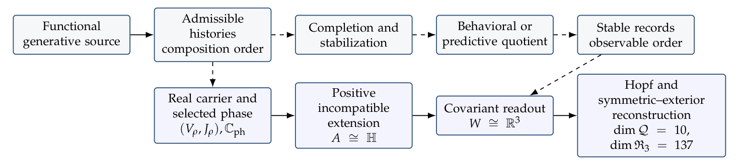
Figure 1 locates the finite reconstruction within the broader program and marks the realization links that are not supplied by its theorems.

3. From Recurrent Source-Order to a Selected Phase Field

3.1. The Source-Order and Its Minimal Real Carrier

Definition 2 (Reversible periodic source-order). The discrete recurrent source is the one-object groupoid \(BC_4\), where

Its source roles are identity, phase step, reversal, conjugate phase step, and return. The continuous refinement is the one-object groupoid \(BS^1_{\mathrm g}\). Neither source contains a metric, angle, orientation, spatial dimension, or pre-given real carrier.

Proposition 2 (Minimal faithful real phase carrier). Let \(\rho:C_4\to GL(V_\rho)\) be a faithful finite-dimensional real representation. Then \(\dim_{\mathbb{R}}V_\rho\geq2\). In minimal dimension, after averaging an inner product and choosing an oriented orthonormal basis,

Thus the minimal carrier is a one-dimensional vector space over the abstract phase field \(\mathbb{C}_{\mathrm{ph}}=\mathbb{R}[i_{\mathrm{ph}}]\), unique up to orthogonal equivalence and phase conjugation.

Proof. A one-dimensional real representation takes values in \(\mathbb{R}^\times\), whose finite-order elements are only \(\pm1\); it cannot represent an element of exact order four faithfully. Thus the dimension is at least two. In dimension two, average any positive inner product over \(C_4\) so that \(\rho(q)\) is orthogonal. An order-four orthogonal map cannot be a reflection and cannot have only the eigenvalues \(\pm1\), so it is rotation by \(\pm\pi/2\) and has the displayed normal form. \(\square\)

Proposition 3 (Minimal faithful continuous phase carrier). Let \(\rho:S^1\to GL(V)\) be a faithful continuous finite-dimensional real representation. Then \(\dim_{\mathbb{R}}V\geq2\). In minimal dimension, after averaging an inner product, \(V\) is an oriented rotation plane and

Equivalently, the minimal faithful real circle carrier is the weight-\(\pm1\) representation and is one-dimensional over \(\mathbb{C}_{\mathrm{ph}}\).

Proof. A continuous homomorphism from the connected group \(S^1\) to \(GL_1(\mathbb{R})=\mathbb{R}^{\times}\) has image in the identity component \(\mathbb{R}_{>0}\); compactness then forces the image to be trivial. Hence no faithful one-dimensional real representation exists. After averaging an inner product, any nontrivial irreducible real summand is a two-dimensional rotation representation of integer weight \(n\). In minimal dimension the representation is one such plane, and faithfulness is equivalent to \(\left\lvert n\right\rvert=1\). \(\square\)

Remark 2 (The plane is expressed, not presupposed). The abstract source is not already a circle embedded in a plane. The plane appears because no real line can carry a faithful square-minus-identity operation. This is the first instance of the source–carrier distinction used throughout the reconstruction.

3.2. Positive-Frequency Selection on a Real Hilbert Flow

Let \(H_{\mathbb{R}}\) be a real Hilbert space and let

be a strongly continuous orthogonal group with skew-adjoint generator \(D\); this is the real form of the standard one-parameter group framework [7,8]. Write

Positive-frequency selection is established in [4, §5, Theorem 4 and Proposition 2] and [5, §§3–4]. We give its spectral proof, including the operator domain and bounded-commutant consequence, so that subsequent arguments require no external selection theorem.

Theorem 1 (Positive-frequency polar selection). Take \(D_{\mathrm{dyn}}\) to have domain \(\operatorname{Dom}(D)\cap H_{\mathrm{dyn}}\). On \(H_{\mathrm{dyn}}\) there is a unique bounded orthogonal complex structure \(J_{D}\) satisfying

Here \(B\) is self-adjoint, \(J_{D}\operatorname{Dom}(B)=\operatorname{Dom}(B)\), and both products in (10) are equalities of closed operators on that common domain. No spectral gap at zero is assumed. Moreover,

Every bounded real-linear operator \(T\) satisfying \(TU(t)=U(t)T\) for all \(t\in\mathbb{R}\) preserves \(H_{\mathrm{dyn}}\) and commutes with \(J_{D}\) there.

Proof. Complexify the flow and write \(U_{\mathbb{C}}(t)=e^{itK}\), so \(D_{\mathbb{C}}=iK\) with \(K\) self-adjoint. For the spectral measure \(E_K\), both \(\operatorname{Dom}(K)\) and \(\operatorname{Dom}(\left\lvert K\right\rvert)\) are characterized by \(\int_{\mathbb{R}}\lambda^2\,d\langle x,E_K(\lambda)x\rangle<\infty\), so their domains agree. Canonical conjugation \(C\) obeys \(CKC=-K\). On the nonzero spectral subspace, \(i\operatorname{sgn}(K)\) therefore commutes with \(C\) and restricts to a real operator \(J_{D}\). Its modulus is one, its square is \(-\operatorname{Id}\), and spectral calculus gives (10), domain preservation, and the displayed Euler formula. Polar-decomposition uniqueness on the support of \(B\) gives uniqueness of \(J_{D}\); only density of \(\operatorname{Ran}B\) is needed.

For the final assertion, the bounded complexification \(T_{\mathbb{C}}\) commutes with every \(e^{itK}\), hence with the spectral projections of \(K\) and every bounded Borel function of \(K\). In particular it commutes with \(E_K(\mathbb{R}\setminus\{0\})\) and \(i\operatorname{sgn}(K)\). Restriction to the real subspace proves both preservation of \(H_{\mathrm{dyn}}\) and \(TJ_{D}=J_{D}T\). This argument does not require \(T\) to be unitary or invertible. \(\square\)

Remark 3 (Zero modes). The phase in Theorem 1 is selected only on the nonzero-frequency subspace. A compatible complex structure on \(H_{\mathrm{fix}}\) requires independent data. No conclusion below uses an unselected zero-mode phase.

3.3. From Selected Phase to Quantum Completion

Eq. (10) makes \(H_{\mathrm{dyn}}\) a complex Hilbert space, with \(J_{D}\) acting as multiplication by \(i_{\mathrm{ph}}\) and the commuting orthogonal flow acting unitarily; compare [6]. A finite operational realization of the two temporal roles can then be specified using the standard dilation and operator-sum framework [9,10]. The additional data are finite complex system and record spaces \(\mathcal H\) and \(\mathcal E\), a unit record state \(|0\rangle\), ordered unitary inner operations \(U_1,\ldots,U_m\) on \(\mathcal H\otimes\mathcal E\), and an orthonormal record basis \((|a\rangle)\). Define

The last identity follows from \(V^*V=\operatorname{Id}\). Assuming the usual trace probability rule, completion into the chosen record basis gives the instrument

Each \(\mathcal I_a\) is completely positive and trace-nonincreasing; \(\Lambda\) is completely positive and trace-preserving (CPTP). For \(p_a>0\), the conditioned state is \(\mathcal I_a(\rho)/p_a\). Thus inner ordering composes amplitudes before completion, while the outer description records outcomes or retains their unconditioned state. With a freshly prepared record space at each cycle, the supplied protocol gives \(\rho_{n+1}=\Lambda(\rho_n)\). The Born rule, the record basis, and this preparation convention are operational premises, not consequences of quaternionic dimension or determinant closure.

Proposition 4 (Exact quantum autonomy criterion). Let \(\mathcal M\) be a CPTP map on the operators of a finite tensor product \(\mathcal H\otimes\mathcal E\), and let \(C=\operatorname{Tr}_{\mathcal E}\). There is a CPTP map \(T\) satisfying \(C\mathcal M=TC\) on all joint states if and only if the Heisenberg adjoint preserves the accessible observable algebra:

In that case \(T\) is unique and is characterized by \(\mathcal M^*(A\otimes\operatorname{Id}_{\mathcal E})=T^*(A)\otimes\operatorname{Id}_{\mathcal E}\).

Proof. The trace adjoint of \(C\) is the injective unital embedding \(C^*(A)=A\otimes\operatorname{Id}_{\mathcal E}\). Taking adjoints of \(C\mathcal M=TC\) gives the stated characterization and hence invariance. Conversely, invariance defines a unique \(T^*\) by restricting \(\mathcal M^*\) to this embedded matrix algebra. Restriction and the inverse algebra identification preserve complete positivity and the identity, so \(T^*\) is unital completely positive and its trace adjoint \(T\) is CPTP. Adjoint duality gives the desired equality. Joint density operators span the operator space, so requiring the identity on states is sufficient. \(\square\)

This is the finite quantum counterpart of Proposition 1. Its subsystem condition is a standard semicausality requirement, excluding influence from the discarded subsystem to the retained one; compare [11]. It is not a new general dilation theorem. Preparing \(|0\rangle\) yields Eq. (12) for that protocol; autonomous evolution from arbitrary correlated joint states requires the stronger invariant-algebra condition. When it fails, the outer description must retain additional memory or specify a preparation rule. These formulas make the quantum realization problem concrete: select the inner operations, stable record observables, and their preparation dynamics. They do not yet derive those selections, tensor-product locality, field commutation relations, or a physical vacuum. The projective spinor and Hopf structures constructed below supply compatible finite kinematics, while the receiver signature remains a separate structural input.

3.4. Oriented Phase Identification

The source carrier, the dynamic Hilbert sector, and the extension algebra are different spaces. Reusing the same symbol \(i\) on all of them would hide a compatibility assumption.

Definition 3 (Oriented phase-identification datum). Given a candidate extension algebra \(A\), an oriented phase-identification datum is

where

are unital real-algebra maps satisfying

Simultaneous phase conjugation precomposes all three maps with \(i_{\mathrm{ph}}\mapsto-i_{\mathrm{ph}}\).

The selected field \(\mathbb{C}_{\mathrm{ph}}\) is therefore one abstract phase field with three explicitly related realizations. It is not identified by notation alone with a gauge group or with a split-complex temporal coordinate.

Remark 4 (Distinct extension assumptions). The second phase used below cannot be interpreted as a rival positive-frequency complex structure for the same real flow: uniqueness in Theorem 1 would force it to coincide with \(J_{D}\). It is an additional order-sensitive operation in an enlarged composition carrier. Its microscopic origin remains a realization problem.

4. Quaternionic Rigidity from Incompatible Phases

The algebraic assumptions in this section are explicit. They are not consequences of positive-frequency selection alone.

Definition 4 (Positive-norm incompatible-phase extension). A positive-norm incompatible-phase extension relative to the datum \(\Phi_{\mathrm{ph}}\) of Definition 3 is a tuple

with the following properties:

1. (H1) \(A\) is a finite-dimensional real unital associative algebra;

2. (H2) \(N:A\to\mathbb{R}\) is a positive-definite quadratic form satisfying

   \[N(xy)=N(x)N(y)\qquad(x,y\in A);\]

3. (H3) \(j_1=\iota_{\mathrm{ph}}(i_{\mathrm{ph}})\) and \(j_1^2=j_2^2=-1\);

4. (H4) \(j_1j_2\neq j_2j_1\).

No anticommutation, quaternionic basis, or spatial axis is assumed.

Lemma 1 (Positive multiplicative norm implies division). Every algebra \(A\) in a positive-norm incompatible-phase extension is a real division algebra.

Proof. Let \(a\neq0\). If \(ab=0\), then

Positivity gives \(N(a)>0\), hence \(N(b)=0\) and \(b=0\). Thus left multiplication by \(a\) is injective. Finite dimensionality makes it surjective, so \(a\) has a right inverse. The same argument for right multiplication gives a left inverse, and associativity shows that the two inverses coincide. \(\square\)

The classical Frobenius theorem states that every finite-dimensional associative real division algebra is isomorphic to \(\mathbb{R}\), \(\mathbb{C}\), or \(\mathbb{H}\) [12]. Standard accounts of the quaternionic and composition-algebra structures may be found in [13,14].

Theorem 2 (Normed quaternionic rigidity). Every positive-norm incompatible-phase extension is isomorphic as a normed real algebra to the standard quaternions:

The anticommutator determines a real scalar

After a normed-algebra automorphism, one may choose a standard quaternionic frame \((i,j,k)\) such that

The parameter \(\eta\) is the overlap of the ordered phase pair and is not fixed by the theorem.

Proof. By Lemma 1, \(A\) is a finite-dimensional associative real division algebra. Frobenius’ classification leaves \(\mathbb{R}\), \(\mathbb{C}\), and \(\mathbb{H}\). The first two are commutative, whereas \(j_1\) and \(j_2\) do not commute. Hence there is a real-algebra isomorphism \(\phi:A\to\mathbb{H}\).

Transport \(N\) to the positive multiplicative quadratic form \(M:=N\circ\phi^{-1}\) on \(\mathbb{H}\). Since \(M(1)=M(1)^2\) and \(M(1)>0\), one has \(M(1)=1\). On the compact group \(\operatorname{Sp}(1)\) of standard unit quaternions, \(M\) is a continuous group homomorphism

Its image is a compact subgroup of \(\mathbb{R}_{>0}\) and is therefore \(\{1\}\). If \(q=ru\) with \(r\geq0\) and \(u\in\operatorname{Sp}(1)\), quadratic homogeneity gives

Thus \(\phi\) is an isometry and \((A,N)\cong(\mathbb{H},N_{\mathbb{H}})\).

A square root of \(-1\) in \(\mathbb{H}\) is a unit imaginary quaternion. Indeed, if \(q=a+v\) with \(a\in\mathbb{R}\) and \(v\in\operatorname{Im}\mathbb{H}\), then \(q^2=-1\) gives

so \(a=0\) and \(\left\lVert v\right\rVert=1\). Inner automorphisms act transitively on the unit sphere of \(\operatorname{Im}\mathbb{H}\), so one may send \(j_1\) to \(i\). Decompose the image of \(j_2\) as \(\eta i+w\) with \(w\perp i\). Noncommutation is equivalent to \(w\neq0\), hence \(\left\lvert \eta\right\rvert<1\). The stabilizer of \(i\) rotates the unit circle in \(i^{\perp}\) transitively and sends \(w/\left\lVert w\right\rVert\) to \(j\). \(\square\)

Corollary 1 (Derived anticommuting frame). Set

Then

Proof. In the normal form of Theorem 2, the elements are the standard imaginary units \(i,j,k\). Transport their multiplication relations back to \(A\). \(\square\)

Remark 5 (Nonredundancy of the assumptions). Associativity excludes the octonionic alternative. Positivity excludes split composition algebras and matrix algebras with isotropic norm. Noncommutation excludes a single complex slice. The theorem does not derive the microscopic existence of the second phase \(j_2\), and it does not select the overlap \(\eta\).

5. Center-Insensitive Records and the Rank-Three Readout

The algebra \(A\cong\mathbb{H}\) is four-dimensional over \(\mathbb{R}\), and its center is one-dimensional. We study real-linear tests that annihilate central offsets. The intended displacement interpretation motivates this choice; it is not a consequence of quaternionic rigidity.

Definition 5 (Center-insensitive covariant records). Let \(A\cong\mathbb{H}\), let \(Z(A)\) be its center, and let

be the connected inner automorphism group, acting on \(A^*\) by

A center-insensitive covariant record space is a nonzero subspace

such that

Its evaluation map and intrinsic readout are

Here a record is an abstract functional \(\ell\), not an observed state generated by a specified procedure. The evaluation map is the entire readout structure assumed at this stage. The quotient \(A/Z(A)\) below is always a quotient of real vector spaces and representations. It is not being used as an algebra quotient.

Lemma 2 (Irreducibility of the quaternionic vector module). The connected inner action of \(\mathbb{H}\) on

is the standard irreducible real representation of \(SO(3)\).

Proof. Conjugation by a unit quaternion preserves the real part and the Euclidean norm of the imaginary part. Its kernel is \(\{\pm1\}\), and the induced homomorphism

is onto; see [15]. Thus the inner action is the standard \(SO(3)\) action on \(\mathbb{R}^3\), which is irreducible over \(\mathbb{R}\). \(\square\)

Theorem 3 (Covariant-readout rigidity). Let \(A\cong\mathbb{H}\) and let \(\mathcal R\) be a center-insensitive covariant record space. Then

and

as real \(G_A\)-modules. In particular, there is no nonzero exactly inner-covariant center-insensitive intrinsic readout of rank one or two.

Proof. Because \(\mathcal R\) annihilates \(Z(A)\), it is a \(G_A\)-invariant subspace of

The representation \(A/Z(A)\) is irreducible by Lemma 2. Its dual is equivalent to it through the invariant Euclidean inner product, hence is irreducible. Since \(\mathcal R\) is nonzero and invariant, it equals all of \(\operatorname{Ann}(Z(A))\).

The common kernel of all functionals in \(\operatorname{Ann}(Z(A))\) is exactly \(Z(A)\). The first isomorphism theorem applied to \(r_{\mathcal R}\) therefore gives

For \(A\cong\mathbb{H}\), the center is \(\mathbb{R}\,1\) and the quotient is naturally represented by the imaginary quaternions, which have real dimension three. \(\square\)

Corollary 2 (Orbit completion). If \(0\neq\ell\in\operatorname{Ann}(\mathbb{R}\,1)\), then the real linear span of the connected-inner orbit of \(\ell\) is all of \(\operatorname{Ann}(\mathbb{R}\,1)\). Thus one nonzero center-insensitive functional, together with the linear span of all its inner reorientations, generates the full rank-three functional space.

5.1. Indexed Readouts and the Missing Realization Maps

If a family \((A_{t_{\mathrm r}},\mathcal R_{t_{\mathrm r}})\) satisfies the local hypotheses at each label, then

This is a family of applications of Theorem 3. A label \(t_{\mathrm r}\) alone supplies neither a completion map nor a chronology, transport, or gluing law. The explicit word-and-transport model below supplies particular algebraic choices, and Proposition 1 states their general descent requirement. To interpret \(W_{t_{\mathrm r}}\) as a spatial displacement space, a realization must provide histories and completed tests, identify their accessible information with \(r_{\mathcal R_{t_{\mathrm r}}}\), and supply calibrated comparison maps

Spatial persistence and particle-like persistence concern those additional data. They are not established by the indexed rank equality. The following explicit example also distinguishes instantaneous readout from the future-preserving quotient of Eq. (2).

5.2. An Instantaneous Record Need Not Preserve Future Records

The rank-three quotient in Theorem 3 concerns a declared family of instantaneous linear tests. The following example shows why a quotient retaining all future tests is a separate construction.

Proposition 5 (Rank-three records and a four-dimensional predictive carrier). Equip \(V=\mathbb{H}\) with its standard real inner product, choose a unit imaginary quaternion \(e_1\), and set

Then \(U\) is an orthogonal flow with generator \(D=J\) and positive polar magnitude \(\left\lvert D\right\rvert=\operatorname{Id}\). The readout \(P\) has rank three, but \(J\) does not descend to \(V/\ker P\). For any \(\varphi\) with \(\sin\varphi\ne0\), let \(S=U(\varphi)\). Then

Writing \(q=a+w\) with \(a\in\mathbb{R}\), \(w=Pq\), and \(w’=PSq\), the reconstruction is

Consequently, a real-linear state representation retaining all these future records for every initial \(q\) requires at least four real dimensions.

Proof. Right multiplication by \(e_1\) is orthogonal and squares to \(-\operatorname{Id}\), hence \(J^*=-J\) and the flow assertions follow. For any linear operator \(T\), the assignment \([q]\mapsto[Tq]\) on \(V/\ker P\) is well defined exactly when \(T(\ker P)\subseteq\ker P\). Here \(\ker P=\mathbb{R}1\) and \(J1=e_1\notin\mathbb{R}1\), so the phase does not descend. If \(Pq=0\), then \(q=a1\) and \(PSq=a\sin\varphi\,e_1\); thus the first intersection in Eq. (16) vanishes, and so does the intersection over all future tests. For imaginary \(w\), \(\operatorname{Im}(we_1)=w\times e_1\) is perpendicular to \(e_1\). Taking the \(e_1\) component of \(PS(a+w)\) proves Eq. (17). The map \(q\mapsto(Pq,PSq)\) is therefore injective. Any linear state encoding through which all future tests factor must itself be injective, giving the dimension bound. \(\square\)

This is an explicitly supplied real-linear readout and flow, not a quantum-ray measurement or a physical completion procedure. Quaternionic conjugation transports both the selected \(e_1\) and the record frame; it need not preserve one fixed \(e_1\)-flow. The example separates instantaneous record rank from the information needed for subsequent prediction without adding a spatial or particle interpretation.

5.3. A Phase-Word Protocol That Generates the Readout Flag

The following finite protocol supplies an explicit algebraic meaning of inner generation. It adds a declared alternating word rule to the phase data, and acquires one linear test per word. The rule and its completion criterion are constitutive choices, not consequences of quaternionic rigidity alone.

Definition 6 (Alternating phase words and prefix records). For the incompatible phase pair \((j_1,j_2)\) of Theorem 2, start with \(a_0=1\) and set

Let \(P:A\cong\mathbb{H}\to W:=\operatorname{Im}\mathbb{H}\) be imaginary projection. At inner depth \(d\), retain the prefix span and the corresponding real tests

Set \(W_0^{\mathrm{word}}=0\). Declare a record cycle complete at the first depth whose tests span \(\operatorname{Ann}(\mathbb{R}1)\); subsequent test acquisition then adds no independent center-insensitive information. This is a rank-completion rule for a finite test protocol, not a physical measurement instrument.

Theorem 4 (Three-step generation and rank-complete readout). Write \(s=\sqrt{1-\eta^2}>0\) and use the derived frame of Corollary 1. The first three projected words are

Consequently,

The protocol completes at depth three, and \(C_3\) induces an isomorphism \(A/\mathbb{R}1\to\mathbb{R}^3\). Thus it realizes the abstract center-insensitive record space of Theorem 3 by explicitly generated tests.

The construction is covariant under simultaneous conjugation of the phase pair and carrier. For a unit quaternion \(h\), with \(g(q)=hqh^{-1}\),

The incomplete rank-one and rank-two test spaces depend on the selected phase pair; only their completed span is independent of that choice.

Proof. Since \(j_1=e_1\) and \(j_2=\eta e_1+s e_2\), quaternion multiplication gives \(a_2=-\eta+s e_3\) and \(a_3=-\eta e_1+s e_2\). The three imaginary parts in Eq. (19) are linearly independent because \(s>0\); their coordinate determinant in \((e_1,e_2,e_3)\) is \(-s^2\). The invariant Euclidean form identifies each prefix span with the span of its test functionals, proving the rank equalities. At depth three, orthogonality to all three vectors is equivalent to \(Pq=0\), so \(\ker C_3=\mathbb{R}1\). The imaginary part of every subsequent word already lies in \(W\), proving saturation. An algebra automorphism transports each word to the corresponding word in the transported pair. Quaternionic conjugation commutes with \(P\) and preserves its Euclidean form, giving both covariance identities. \(\square\)

The theorem generates independent readout directions by ordered operations; it does not construct the ambient quaternion algebra in the absence of a previously specified carrier. Forgetting orientations on the proper prefix subspaces gives precisely the kind of complete flag used in Definition 8. The full ordered phase pair contains more information than that flag; subsequent receiver results use only the flag. No elapsed time, physical spatial metric, or Lorentzian signature follows from the prefix index. The finite construction grounds the proposed inner-generation role at the level of algebraic tests.

Corollary 3 (Order-sensitive and stable readout generation). Under Theorem 4, write \([A,A]_{\mathrm{span}}:=\operatorname{span}_{\mathbb{R}}\{ab-ba:a,b\in A\}\). The generated directions satisfy

With the inherited Euclidean norm on \(W\) and the standard norm on the three test values, every \(w\in W\) obeys

In particular, if \(\left\lvert \eta\right\rvert\leq1-\delta\) with \(\delta>0\), the inverse readout has operator norm at most \(\delta^{-1/2}\).

Proof. The displayed word formulas and \([j_1,j_2]=2s e_3\) give the first identities. Every quaternionic commutator is imaginary, while \([e_2,e_3]=2e_1\), \([e_3,e_1]=2e_2\), and \([e_1,e_2]=2e_3\) span all of \(W\). In the orthonormal frame \((e_1,e_2,e_3)\), the rows of \(C_3|_W\) are \((1,0,0)\), \((0,0,s)\), and \((-\eta,s,0)\). Their Gram matrix has eigenvalues \(1-\left\lvert \eta\right\rvert\), \(1-\eta^2\), and \(1+\left\lvert \eta\right\rvert\), proving both norm bounds and the inverse estimate. \(\square\)

Thus the inner protocol generates a complete, stably recoverable readout from incompatible phase operations and their order-sensitive difference; recovery becomes ill-conditioned as the phases approach commutation. This establishes algebraic readout emergence, while its interpretation as physical displacement still requires calibrated persistent records and comparison between completed realizations.

5.4. An Explicit Compatible Outer Flow

Proposition 6 (Outer transport compatible with inner generation). Fix \(\Omega\in\operatorname{Im}\mathbb{H}\), put \(h(t)=\exp(t\Omega/2)\), and define

Then \(U_{\Omega}\) preserves \(\ker P=\mathbb{R}1\) and

For the fixed phase-pair protocol of Definition 6, \(C_3=L P\) with an invertible \(L:W\to\mathbb{R}^3\); hence its completed coordinates have the autonomous flow \(L T_{\Omega}(t)L^{-1}\). If the phase pair also evolves by \(j_r(t)=U_{\Omega}(t)j_r(0)\), every prefix word and generated subspace is transported by the same conjugation, so inner acquisition and outer transport are compatible at each depth.

Proof. Conjugation fixes real scalars and preserves imaginary parts, norms, and orientation, proving the descent and rotation statements. Differentiation gives \(\frac12[\Omega,w(t)]=\Omega\times w(t)\). The invertibility of \(L\) follows from Theorem 4. Finally, \(U_{\Omega}(t)(qj)=U_{\Omega}(t)(q)U_{\Omega}(t)(j)\); induction on word length gives the asserted compatibility. \(\square\)

Together, Theorem 4 and Proposition 6 provide a finite dual-time model: the inner protocol successively makes independent tests available, completion retains the rank-three readout, and the specified outer flow compares completed states. With a transported test frame the recorded components are covariant invariants; with a fixed test frame they follow the displayed nontrivial outer flow. This distinction prevents a change of record frame from being mistaken for additional dynamics. The generator \(\Omega\) and the outer time parameter are supplied, not derived from the word grammar. A physical realization must still select the generator, time calibration, measurement process, and spacetime interpretation. By contrast, the right-multiplication flow in Proposition 5 fails the descent criterion and requires a larger predictive carrier. The two examples show exactly which compatibility condition separates closed outer dynamics from evolution that depends on hidden memory.

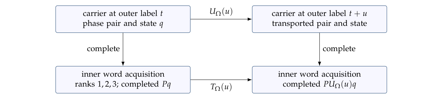
The commuting readout diagram in Figure 2 summarizes this compatibility: applying the supplied outer transport before readout gives the same completed coordinates as applying the induced evolution after readout.

5.5. Euclidean, Rotational, and Spin Structures

Theorem 5 (Quaternionic Euclidean readout). On \(W:=\operatorname{Im}\mathbb{H}\), quaternionic multiplication has the decomposition

where

The form \(\langle\cdot,\cdot\rangle\) is positive definite, the cross product is alternating and orientation-compatible, and

Every invariant positive-definite symmetric bilinear form on \(W\) is a positive scalar multiple of \(\langle\cdot,\cdot\rangle\).

Proof. For imaginary quaternions, the scalar and imaginary parts of the product give Eq. (25). The standard norm makes the displayed bilinear form Euclidean. Every real algebra automorphism of \(\mathbb{H}\) is inner and acts by an orientation-preserving isometry on \(W\), giving \(\operatorname{Aut}_{\mathbb{R}\text{-alg}}(\mathbb{H})\cong SO(3)\). If \(g’\) is another invariant positive form, write \(g'(u,v)=\langle Tu,v\rangle\) for a positive self-adjoint \(T\). Invariance implies that \(T\) commutes with the irreducible standard \(SO(3)\) action, so \(T=c\operatorname{Id}\) for some \(c>0\). \(\square\)

Proposition 7 (Minimal phase-compatible spinor). Let \(\mathbb{C}_{\mathrm{ph}}=\operatorname{span}_{\mathbb{R}}\{1,e_1\}\) be the selected complex slice and let \(p_{\mathbb{C}_{\mathrm{ph}}}:\mathbb{H}\to\mathbb{C}_{\mathrm{ph}}\) be orthogonal projection for the standard quaternionic norm. Regard \(\mathbb{H}\) as a right \(\mathbb{C}_{\mathrm{ph}}\)-vector space and define

Then \((S,h)\), with \(S:=\mathbb{H}_{\mathbb{C}_{\mathrm{ph}}}\), is a two-dimensional \(\mathbb{C}_{\mathrm{ph}}\)-Hermitian space and

The unit quaternions act on \(S\) as \(SU(2)\), and their conjugation action on \(W\) gives the double cover

Proof. Using the anticommuting unit \(e_2\) of Corollary 1, every quaternion is uniquely

Hence \((1,e_2)\) is a right \(\mathbb{C}_{\mathrm{ph}}\)-basis and \(\dim_{\mathbb{C}_{\mathrm{ph}}}S=2\). Projection onto the selected slice is \(\mathbb{C}_{\mathrm{ph}}\)-bimodular, so \(h\) is conjugate-linear in the first variable and linear in the second. By the normed-algebra conclusion of Theorem 2,

for \(s\neq0\).

In the right basis \((1,e_2)\), left multiplication by \(q=a+e_2b\) has matrix

In particular, the matrices of \(1,e_1,e_2,e_3\) are

They are linearly independent over \(\mathbb{C}_{\mathrm{ph}}\) and therefore form a basis of \(M_2(\mathbb{C}_{\mathrm{ph}})\). Hence

is an isomorphism of complex algebras. Eq. (26) shows that a unit quaternion acts unitarily with complex determinant one. Conversely, every matrix in \(SU(2)\) has the form displayed in (26) with \(a\overline a+b\overline b=1\), so the image is all of \(SU(2)\). The conjugation action on \(W\) has kernel \(\{\pm1\}\) and image \(SO(3)\). \(\square\)

Proposition 8 (Qubit state geometry of the readout). For \(w\in W\), set \(\sigma(w)=i_{\mathrm{ph}}L_w\) on the spinor \(S\), where \(L_w\) is left quaternion multiplication. Then \(\sigma(w)\) is Hermitian and traceless, \(\sigma(w)^2=\left\lVert w\right\rVert^2\operatorname{Id}\), and

is a density matrix exactly when \(\left\lVert w\right\rVert\leq1\). For a unit \(n\in W\), \(P_n=\tfrac12(\operatorname{Id}+\sigma(n))\) is a rank-one projector and

Quaternionic conjugation intertwines spatial rotations with unitary conjugation of these matrices.

Proof. For imaginary \(w\), \(L_w^*=-L_w\), \(\operatorname{Tr}L_w=0\), and \(L_w^2=-\left\lVert w\right\rVert^2\operatorname{Id}\). Hence the eigenvalues of \(\rho_w\) are \((1\pm\left\lVert w\right\rVert)/2\). The quaternion product gives \(\operatorname{Tr}(\sigma(w)\sigma(n))=2\langle w,n\rangle\), proving the probability formula; conjugation gives covariance. \(\square\)

The formula is the usual qubit Born probability once density matrices and projectors are given their quantum operational meaning. It exhibits an exact state-space realization of the rank-three geometry; identifying a Bloch vector with physical displacement is an additional correspondence.

Remark 6 (Meaning of local three-dimensional reconstruction). The preceding results identify an abstract real rank-three readout module, with Euclidean metric, orientation, cross product, rotation action, and spin cover. A physical displacement interpretation requires the correspondence described above. It does not by itself construct a global spatial manifold or spacetime. §11.1 adds calibrated histories to obtain a conditional local causal geometry. Persistent records, physical calibration, transport, gluing, and coordination remain realization requirements.

5.6. An Operational Word Measurement

The word tests and the spinor state space admit a common quantum implementation. The trace probability rule and independent state preparations are supplied operational premises. As in informationally complete tomography [16], reconstruction concerns an outcome distribution over many copies, not simultaneous sharp values of incompatible observables on one copy. Put \(s=\sqrt{1-\eta^2}\) and

Here \(C=C_3|_W\) is invertible by Theorem 4; the outcome-coordinate basis \((\epsilon_r)\) of \(\mathbb{R}^3\) is distinct from the quaternionic frame \((e_r)\).

Proposition 9 (Informationally complete word instrument). For \(m=(r,\varepsilon)\) in \(\mathcal M=\{1,2,3\}\times\{+1,-1\}\), define

These maps form a completely positive instrument whose sum is trace preserving. For \(\rho_w=\frac12(\operatorname{Id}+\sigma(w))\), \(\left\lVert w\right\rVert\leq1\),

Thus the outcome law determines the state. The instrument is covariant under simultaneous quaternionic conjugation of the phase pair and state.

Proof. Since \(\left\lVert v_r\right\rVert\leq1\), the eigenvalues \(\pm\left\lVert v_r\right\rVert\) of \(\sigma(v_r)\) make every effect positive. Each pair sums to \(\operatorname{Id}/3\), hence \(\sum\limits_mK_m^*K_m=\operatorname{Id}\). The trace identities of Proposition 8 give (28), and invertibility of \(C\) gives informational completeness. Conjugation transports each Pauli operator unitarily; functional calculus transports its positive square root as well. \(\square\)

Equivalently, choose \(r\) uniformly and measure \((\operatorname{Id}\pm\sigma(v_r))/2\). The second binary measurement is unsharp unless \(\eta=0\). The equal sampling weights and unrescaled word vectors are part of this particular design.

5.7. An Autonomous Recorder and Its All-Attempt Statistical Cost

We compile the instrument into a time-independent finite Hamiltonian, using the history-clock construction and engineered spin transfer [17,18]. Autonomy means that no Hamiltonian coefficient is switched during a run. Preparation, the loaded measurement, clock calibration, and one final interrogation remain specified operations.

Let \(\mathcal H_R=\mathbb{C}_{\mathrm{ph}}^6\) have outcome basis \((|m\rangle)\) and a unit ready vector \(|d_0\rangle\). The isometry \(\psi\mapsto\sum\limits_mK_m\psi\otimes|m\rangle\) extends to a unitary \(U_{\mathrm{wr}}\) on \(S\otimes\mathcal H_R\) with

Indeed, \(\sum\limits_mK_m^*K_m=\operatorname{Id}\) preserves inner products on the ready subspace, and completing orthonormal bases extends the isometry unitarily; this is the finite dilation mechanism of [9,10]. A separate bit \(\mathcal H_F=\mathbb{C}_{\mathrm{ph}}^2\) distinguishes a blank apparatus from every valid datum. On \(\mathcal H_{\mathrm{work}}=S\otimes\mathcal H_R\otimes\mathcal H_F\) put

Choose \(L\geq1\), \(\omega>0\), and a clock basis \(|j\rangle\), \(0\leq j\leq L\). Set \(V_1=U_g\), \(V_j=\operatorname{Id}\) for \(j\geq2\), \(G_0=\operatorname{Id}\), and \(G_j=V_j\cdots V_1=U_g\) for \(j\geq1\). These are apparatus stages, not the three acquisition depths of the word protocol.

Theorem 6 (Exact recorder, completion certificate, and finite capture window). The time-independent self-adjoint Hamiltonian

acts on a space of dimension \(24(L+1)\). From \(|0\rangle\langle0|_C\otimes\rho_0\), tracing out the clock at time \(t\) gives

On the invariant prepared-history subspace \(\mathcal L_{\mathrm{init}}=\bigoplus_{j=0}^L|j\rangle\otimes G_j\mathcal B\), where \(\mathcal B=S\otimes\operatorname{span}\{|d_0\rangle\}\otimes\operatorname{span}\{|0\rangle_F\}\), the physical completion bit equals the projector onto clock stages \(j\geq1\). Reading the bit and, only when it is one, the data register produces

Conditioned on completion, the instrument is exactly (27). At \(t_*:=\pi/\omega\) completion is certain. At \(t=t_*+u\), both the work-state trace distance and the total variation distance between the recorded outcome distributions from the completed values equal \(\sin^{2L}(\omega u/2)\). Their worst value on \(|u|\leq\Delta\leq\pi/\omega\) is \(\sin^{2L}(\omega\Delta/2)\).

Proof. Let \(D=\sum\limits_{j=0}^L|j\rangle\langle j|\otimes G_j\). Direct multiplication gives \(D^*H_{\mathrm{aut}}D=H_C\otimes\operatorname{Id}\), where \(H_C\) is (30) with every \(V_j\) replaced by \(\operatorname{Id}\). Identify its clock with the symmetric subspace of \(L\) two-level factors: \(H_C=(\hbar\omega/2)\sum\limits_{r=1}^L X_r\) there. The amplitude at stage \(j\) is

Thus the full state is \(\sum\limits_{j,k}a_j\overline{a_k}|j\rangle\langle k|\otimes G_j\rho_0G_k^*\). Its clock trace gives (31), since every nonzero stage has the same completed work state. Dressing maps the invariant space \(\mathcal H_C\otimes\mathcal B\) to \(\mathcal L_{\mathrm{init}}\). On its stage-zero summand the bit is zero; on every other summand it is one. This proves the certificate and (32). The ready and final states have orthogonal bit supports, so their mixture has trace distance \(1-p(t)\) from \(\rho_{\mathrm{fin}}\); the distance between the recorded outcome distributions is the same blank mass. Substituting \(t_*+u\) and using monotonicity on the stated window proves the remaining assertions. \(\square\)

Corollary 4 (Exact all-attempt risk and conditional phase selection). Run the recorder on \(n\geq1\) independently prepared copies of \(\rho_w\), using fresh ready apparatus states and the same separately calibrated completion probability \(p=p(t)>0\). For each attempt define \(Y=0\) on a blank and \(Y=3\varepsilon\epsilon_r/p\) on outcome \((\mathrm{complete},r,\varepsilon)\). Then

The estimator is unbiased; \(n\) counts all attempts, including blanks. At fixed \(p,n\), its worst-case risk is \(9/[np(1-\eta^2)]\) and is uniquely minimized within this design by \(\eta=0\), equivalently \(j_1j_2=-j_2j_1\). For \(p=1\) this reduces to the exact ideal readout risk.

Proof. Eq. (32) gives \(\mathbb E_wY=Cw\) and \(\mathbb E_w(YY^T)=3I_3/p\). Independence makes the risk

The Gram eigenvalues in Corollary 3 give \(\operatorname{Tr}((C^TC)^{-1})=3/(1-\eta^2)\). The worst input is \(w=0\), and \(1/(1-\eta^2)\) is uniquely minimized at zero. \(\square\)

The formula treats \(p\) as known exactly. Calibration uncertainty, including that of an independent estimate of \(p\), contributes additional error and is not included in the displayed risk. Euclidean projection of \(\widehat w_n\) onto the Bloch ball can only decrease its squared error, but then (33) is an upper bound. The optimization fixes equal index weights, the unrescaled word vectors, the estimator, and the clock parameters; it does not establish optimality over arbitrary measurements or an unconditional derivation of anticommutation. At this optimum \(j_1j_2=-j_2j_1\), so the two opposite-order unitary words differ only by a global phase and induce identical conjugation channels. Distinguishing those orders requires a supplied coherent reference or another interference protocol; the tomography optimum alone is not an order witness.

The engineered clock has bandwidth \(B_{\mathrm{clk}}=\hbar\omega L\) and \(\left\lVert H_{\mathrm{aut}}\right\rVert=\hbar\omega L/2\). Its capture error is \(O(u^{2L})\), but increasing \(L\) at fixed bandwidth lengthens \(t_*=\pi\hbar L/B_{\mathrm{clk}}\). These are costs of this construction, not universal speed limits. Moreover \(e^{-i_{\mathrm{ph}}(2\pi/\omega)H_{\mathrm{aut}}/\hbar}=(-1)^L\operatorname{Id}\), so the closed device returns to its blank preparation. A finite-Hamiltonian expectation is analytic in time: if its completion probability were constant on an open interval, it would be constant everywhere. An initially blank finite closed recorder therefore cannot develop an exact permanent completion plateau. The result concerns one interrogation per fresh run, not irreversible storage or a reset mechanism. The bit certifies execution of a supplied dilation; the trace rule, ready states, unitary extension, and engineered couplings remain inputs. The construction does not assert a two-body or spatially local implementation. An autonomous total Hamiltonian also does not ensure autonomous reduced dynamics from arbitrary correlated initial states.

6. Projective Phase Geometry, Hopf Degree, and Bundle-Role Separation

The quaternionic closure supplies a complex spinor doublet, a projective sphere, and a canonical principal circle bundle relative to the selected phase orientation; standard background is given in [19,20]. These statements concern a bundle over projective spinor space. They do not yet identify an electromagnetic bundle over spacetime, a photon-polarization bundle, or a \(\mathrm{Spin}^c\) determinant line.

6.1. Projective Directions and the Hopf Fibration

Let

The group \(U(1)_{\mathrm{ph}}\) acts freely on the right of \(\mathbb S(S)\). Let \(S(W)\) denote the unit sphere in the Euclidean readout \(W\).

Theorem 7 (Direction–spinor correspondence and Hopf fibration). The map

is surjective and is constant exactly on the right \(U(1)_{\mathrm{ph}}\)-orbits. It therefore induces an \(SU(2)\)-equivariant diffeomorphism

Consequently,

is the Hopf principal circle bundle in the selected phase convention.

Proof. For unit \(\psi\), conjugation preserves the imaginary-quaternion unit sphere. If \(z\in U(1)_{\mathrm{ph}}\), then \(z\) commutes with \(e_1\), so \(\beta(\psi z)=\beta(\psi)\). Conversely, \(\beta(\psi)=\beta(\phi)\) implies that \(\phi^{-1}\psi\) stabilizes \(e_1\) under conjugation. The stabilizer of \(e_1\) in \(\operatorname{Sp}(1)\) is exactly \(U(1)_{\mathrm{ph}}\). Surjectivity follows from transitivity of quaternionic conjugation on \(S(W)\). \(\square\)

6.2. The Positive Hopf Line and Its Chern Degree

Let \(\mathcal T\to\mathbb P_{\mathbb{C}_{\mathrm{ph}}}(S)\) be the tautological complex line bundle. With the complex orientation on \(\mathbb P_{\mathbb{C}_{\mathrm{ph}}}(S)\cong\mathbb{CP}^1\), define

We use the curvature convention \(F_\nabla:=\nabla^2\in\Omega^2(X;i\mathbb{R})\) for a unitary line connection, with local form \(\nabla=d+A\) and curvature \(F_\nabla=dA\). Thus the real form \(f_\nabla:=iF_\nabla\) satisfies \(c_1(L)_{\mathrm{dR}}=[f_\nabla/(2\pi)]=[iF_\nabla/(2\pi)]\).

Theorem 8 (Primitive Hopf degree). The positive Hopf line satisfies

Equivalently, for any unitary connection \(\nabla_{\mathrm H}\) on \(\mathcal L_{\mathrm H}\) with curvature \(F_{\mathrm H}\),

Proof. On the standard affine charts \(U_0,U_1\) with coordinate \(w=z_1/z_0\), the tautological frames satisfy \(t_1=w^{-1}t_0\). The dual frames therefore satisfy \(t_1^*=w t_0^*\). Their unitary normalizations have transition \(w/\left\lvert w\right\rvert\), equal to \(w\) on the equator. In these frames the connection forms obey \(A_1=A_0+w^{-1}dw\) along the equator, so Stokes’ theorem gives \(\int_{\mathbb{CP}^1}F_{\mathrm H}=-\oint_{\left\lvert w\right\rvert=1}w^{-1}dw=-2\pi i\). Hence \(\frac{i}{2\pi}\int F_{\mathrm H}=1\), consistent with the positive degree of \(\mathcal T^*\) and (35); see [19,20]. \(\square\)

Theorem 9 (Circle characters and the Chern-degree lattice). Every continuous character \(\chi:U(1)\to U(1)\) is \(\chi_q(z)=z^q\) for a unique \(q\in\mathbb{Z}\). Define

Then

The least nonzero absolute degrees are \(q=\pm1\).

Proof. Lift \(\chi\) through \(\exp:\mathbb{R}\to U(1)\). The lift is a continuous additive map \(t\mapsto qt\). Periodicity under \(t\sim t+2\pi\) forces \(q\in\mathbb{Z}\). The Chern-degree formula follows from additivity under tensor product and sign reversal under dualization. \(\square\)

Definition 7 (Primitive source-monopole interpretation). A source-monopole realization means that the first nontrivial projective phase line downstream of the generative source is interpreted by a line of Hopf degree \(\pm1\). This does not place the source in empirical spacetime or identify it with a detectable magnetic monopole.

Proposition 10 (Topology does not determine coupling strength). Let \((X,h)\) be a closed oriented smooth Riemannian manifold of dimension at least two, and fix a smooth Hermitian line bundle \(L\to X\). For a unitary connection \(\nabla_A\), put

With the Hodge star \(*_h\) determined by \(h\) and the orientation, the family of kinetic functionals

is nonnegative and has the same underlying bundle for every \(g\). The factor \(1/(2g^2)\) gives the component normalization \((4g^2)^{-1}\int_X(f_A)_{\mu\nu}(f_A)^{\mu\nu}\,d\operatorname{vol}_h\). Thus bundle topology does not determine this continuous kinetic coefficient; no electromagnetic identification is needed for this conclusion.

Proof. The identity \(f_A\wedge *_h f_A=\lvert f_A\rvert_h^2\,d\operatorname{vol}_h\) proves nonnegativity. Varying \(g\) changes only the coefficient: \(L\), its transition functions, and \(c_1(L)\in H^2(X;\mathbb{Z})\) remain fixed. The real class \([f_A/(2\pi)]=[iF_A/(2\pi)]\) is the image of \(c_1(L)\) in de Rham cohomology; this real class need not detect torsion. Consequently the Chern degree and character weights are insensitive to the kinetic normalization. \(\square\)

6.3. \(\mathrm{Spin}^c\) and the Factor-of-Two Distinction

Proposition 11 (\(\mathrm{Spin}^c(3)\) character bookkeeping). Write, following the standard convention in [21],

Let \(\Delta:\mathrm{Spin}(3)\to SU(2)\) be the complex spin representation. Then

is a well-defined representation on \(\mathbb{C}^2\), and

Consequently, the conventional \(\mathrm{Spin}^c\) determinant character has central weight two. The assignment \([g,z]\mapsto z\) is not a well-defined one-dimensional character of \(\mathrm{Spin}^c(3)\), because \((g,z)\) and \((-g,-z)\) represent the same class. A weight-one electromagnetic matter line therefore cannot be extracted from a \(\mathrm{Spin}^c\) structure alone; identifying an external matter line \(M\) with a square root of the determinant line, \(M^{\otimes2}\cong L_{\det}\), is additional structure.

Proof. The pair \((-1,-1)\) acts as \((-1)\Delta(-1)=(-1)(-I)=I\), so the representation descends to the quotient. Since \(\Delta(g)\in SU(2)\), its determinant is one, and scalar multiplication by \(z\) on a two-dimensional complex spinor has determinant \(z^2\). \(\square\)

Proposition 12 (Classifying-space discipline). Let \(X\) be a CW complex, and let \(H^2(X;\mathbb{Z})\) denote singular cohomology with constant integer coefficients. Isomorphism classes of ordinary complex line bundles on \(X\) are classified by

If \(\dim X\leq2\), a representative may be chosen to factor through the \(2\)-skeleton \(\mathbb{CP}^1\hookrightarrow\mathbb{CP}^{\infty}\). For a topological groupoid \(\mathcal E\), the same assertion applies to ordinary line bundles on a chosen classifying space \(B\mathcal E\) when that space is a CW complex. No classification of \(\mathcal E\)-equivariant line bundles is asserted here.

Proof. CW complexes are paracompact, so their line bundles admit classifying maps to \(BU(1)\simeq\mathbb{CP}^{\infty}\). This space is a \(K(\mathbb{Z},2)\), giving the singular-cohomology identification. Cellular approximation gives the factorization through \(\mathbb{CP}^1\) for a two-dimensional CW base. The groupoid sentence is the same ordinary bundle classification applied to the explicitly specified CW base \(B\mathcal E\); see [22,23]. \(\square\)

The distinct bases, fibers, and representation weights are compared in Table 2. Keeping these roles separate specifies which additional realization maps are needed before the projective Hopf construction can be related to an electromagnetic matter line.

Table 2. Bundle roles that must not be identified without a realization map.

Object	Base and structural role	Additional requirement for physics
Hopf line \(\mathcal L_{\mathrm H}\)	\(\mathbb P_{\mathbb{C}_{\mathrm{ph}}}(S)\cong\mathbb{CP}^1\); projective spinor phase and Chern degree.	A classifying map from the physical base and a connection comparison.
Polarization/Berry line	A parameter or Poincaré sphere of photon states.	A bundle-and-connection realization, not merely an abstract \(S^2\) identification.
Weight-one matter line	Electron record, parameter, or spacetime base.	A physical matter representation and target-blind orientation rule.
\(\mathrm{Spin}^c\) determinant line	A \(\mathrm{Spin}^c\) base; the determinant character has central weight two.	Existence and choice of a square-root matter line, if required, plus an electromagnetic identification.
Electromagnetic \(U(1)\) bundle	Physical spacetime or an effective configuration base.	Gauge and matter action, renormalization convention, and empirical matching.

Problem 1 (Polarization realization). Construct a classifying map and unitary bundle morphism from the relevant physical polarization base to the Hopf class, using the Pancharatnam–Berry framework [24–26], and prove compatibility of the Hermitian structures and connections. Abstract isomorphism of two copies of \(\mathbb{CP}^1\) is not sufficient.

7. Unital Carrier Envelope and Filtered Quadratic Closure

The readout quotient removes the scalar center. The reconstruction signature studied here restores a distinguished scalar channel before forming pair data. This is a chosen retention rule: it is motivated by retaining the identity coefficient of the original carrier, but does not follow from the quotient theorem.

Principle 13 (Unital carrier-envelope restoration). The displacement readout is the center-insensitive quotient \(W\cong\mathbb{H}/\mathbb{R}\mathbf1\), but reconstruction closure acts on the complete unital carrier envelope

as a real vector space and \(SO(W)\)-module. The summand \(\mathbb{R}\mathbf1\) retains the carrier identity. Interpreting it as persistence or null-displacement data is optional and requires a realization; it is not counted as a readout direction.

Definition 8 (Complete flag in an oriented carrier). Let

be a complete flag in the already oriented Euclidean space \(W\). The proper subspaces \(W_1\) and \(W_2\) carry no chosen orientations. We use “flag in oriented \(W\)” in precisely this sense throughout. An adapted positively oriented orthonormal basis can be chosen for calculations, but is not part of the flag datum. Its four determinant-one diagonal sign changes stabilize the flag; the resulting groupoid is specified in Proposition 20. Define

Then \(\dim_{\mathbb{C}_{\mathrm{ph}}}\mathcal U_d=d+1\), \(\mathcal U_d/\mathcal U_{d-1}\cong\mathbb{C}_{\mathrm{ph}}\) for \(d\geq1\), and \(E_3=E\). Give \(E_d\) the Euclidean inner product for which \(\mathbf1\perp W_d\) and \(\left\lVert \mathbf 1\right\rVert=1\), and give \(\mathcal U_d\) its induced Hermitian form.

Proposition 13 (Real quadratic data and complex base change). For every finite-dimensional real vector space \(E_d\), the map

is a natural \(\mathbb{C}_{\mathrm{ph}}\)-linear isomorphism. Hence the complex symmetric square below may be read as the complexification of all real symmetric quadratic carrier data.

Proof. The displayed map is well defined and \(\mathbb{C}_{\mathrm{ph}}\)-linear. Complex bilinearity shows that every elementary symmetric tensor on the right lies in its image. Both sides have complex dimension \(n(n+1)/2\) when \(n=\dim_{\mathbb{R}}E_d\), so the map is an isomorphism. Naturality follows from functoriality of scalar extension and symmetric powers. \(\square\)

Proposition 14 (Symmetric-square universal property). For complex vector spaces \(U\) and \(X\), composition with the canonical symmetric bilinear map \(U\times U\to\operatorname{Sym}^2_{\mathbb{C}_{\mathrm{ph}}}U\) gives a natural bijection

Thus \(\operatorname{Sym}^2_{\mathbb{C}_{\mathrm{ph}}}U\) is the free linear receiver of complex-bilinear symmetric pair data on \(U\); see also [27].

Proof. The tensor-product universal property identifies bilinear maps \(U\times U\to X\) with linear maps \(U\otimes U\to X\). A bilinear map is symmetric exactly when it annihilates the subspace generated by \(u\otimes v-v\otimes u\), so it factors uniquely through \(\operatorname{Sym}^2U\). \(\square\)

Principle 14 (Free quadratic-pair completion). At each depth, the closure sector retains all unordered complex-bilinear pair data on \(\mathcal U_d\) and imposes no relations beyond symmetry. Equivalently, by Proposition 13, it retains the complexification of all real symmetric quadratic pair data on \(E_d\). The corresponding free receiver is \(\operatorname{Sym}^2_{\mathbb{C}_{\mathrm{ph}}}(\mathcal U_d)\). The motivation is informational: this retains every symmetric bilinear test, including mixed identity–vector terms, without choosing a basis or imposing an unmotivated relation among those tests. Symmetry expresses the stipulated irrelevance of pair order. Bilinearity, pair degree two, and absence of further relations remain assumptions; neither covariance nor positivity alone selects them. The theorem below determines their consequences.

Definition 9 (Filtered quadratic closure). Set \(\mathcal Q_{-1}=0\) and

The inclusions \(\mathcal U_{d-1}\hookrightarrow\mathcal U_d\) induce inclusions \(\mathcal Q_{d-1}\hookrightarrow\mathcal Q_d\). Symmetric powers carry the standard induced Hermitian forms.

Theorem 10 (Quadratic filtration theorem). For \(d=0,1,2,3\),

Hence

and

The full closure object \(\mathcal Q\) depends only on \(W\), the unital envelope, and the selected phase field. The filtered objects form an equivariant family over the flag groupoid in oriented \(W\) defined in Proposition 20.

Proof. Since \(\dim_{\mathbb{C}_{\mathrm{ph}}}\mathcal U_d=d+1\),

Every inclusion of finite-dimensional vector spaces splits, so the induced symmetric-square map is injective. Therefore

At \(d=3\) this gives \(\dim\mathcal Q=\binom52=10\). \(\square\)

Proposition 15 (\(SO(3)\)-type decomposition of the closure and terminal branch). Let \(W_{\mathbb{C}_{\mathrm{ph}}}:=\mathbb{C}_{\mathrm{ph}}\otimes_{\mathbb{R}}W\). With \(\mathbf 1\), \(\mathbf 3\), and \(\mathbf 5\) denoting the trivial, vector, and traceless symmetric rank-two complex \(SO(3)\) representations, respectively,

Moreover,

Thus the dimensions \(10\) and \(7\) carry nontrivial rotational type data rather than being featureless counts.

Proof. The unital envelope decomposes as a scalar plus the standard vector representation. Hence

For the branch object, \(\Lambda^1\mathbf3\cong\mathbf3\), the oriented Hodge star gives \(\Lambda^2\mathbf3\cong\mathbf3\), and \(\Lambda^3\mathbf3\cong\mathbf1\). \(\square\)

Remark 7 (What the number ten does and does not express). The ladder \((1,2,3,4)\) is the associated-graded dimension sequence of one filtered quadratic object, and \(10\) is the dimension of its full closure. No independent positive scalar is introduced. The use of \(E=\mathbb{R}\mathbf1\oplus W\) and of the free symmetric receiver remains explicit constitutive content; alternatives are audited in §Appendix A.

Remark 8 (Ten quadratic channels and an optional decimal encoding). The quadratic filtration derives the cumulative dimensions \(1,3,6,10\), with increments \(1,2,3,4\), under the free quadratic-pair rule. These differ from the rotation-sector dimensions \(1+1+3+5\) in Proposition 15. Relative to a complete orthogonal flag, the four unital-envelope lines \(L_0=\mathbb{C}_{\mathrm{ph}}\mathbf1,L_1,L_2,L_3\) determine ten pair lines \(L_i\odot L_j\), \(0\leq i\leq j\leq3\). A convention assigning one primitive symbol to each pair channel requires ten symbols. Decimal place value is an optional encoding of these labels: block codes need only satisfy \(b^k\geq10\), and the vector space itself has continuously many states. The channel count and receiver rank are independent of numeral notation; the channel lines depend on the flag.

Hypothesis 1 (Dynamical quadratic-sector realization). When a concrete spectral interpretation is required, the selected positive-frequency dynamical theory contains a finite \(\mathbb{C}_{\mathrm{ph}}\)-linear invariant sector isomorphic to \(\mathcal Q\), together with the induced filtration or an equivalent grading. The abstract dimension theorem does not depend on this realization hypothesis.

Proposition 16 (Rank-one operator realization of the associated-graded ladder). Let \(K=\bigoplus_{d=0}^{3}K_d\) be a finite-dimensional graded complex space with \(\dim K_0=1\). Suppose an outer-update map \(T_{\mathrm o}\) satisfies \(T_{\mathrm o}(K_d)\subseteq K_{d+1}\), its restriction \(K_d\to K_{d+1}\) is injective for \(d<3\), and

Then \(\dim_{\mathbb{C}_{\mathrm{ph}}}K_d=d+1\) and \(\dim_{\mathbb{C}_{\mathrm{ph}}}K=10\). In particular, if an inner-update operator \(T_{\mathrm i}\) has commutator \(\Omega=[T_{\mathrm i},T_{\mathrm o}]\) with

and the displayed quotient is one-dimensional, the operator module realizes the same \((1,2,3,4)\) dimensions as the associated-graded pieces \(\mathcal G_d\).

Proof. Injectivity gives \(\dim T_{\mathrm o}(K_d)=\dim K_d\). The one-dimensional quotient therefore implies \(\dim K_{d+1}=\dim K_d+1\). Induction from \(\dim K_0=1\) yields the stated ladder and total dimension. \(\square\)

Remark 9 (Scope of the operator route). Proposition 16 supplies an optional dynamical realization of the associated-graded ladder; it does not derive the symmetric receiver \(\mathcal Q\), the exterior branch law, or the homogeneous reconstruction recursion. Bare noncommutation \([T_{\mathrm i},T_{\mathrm o}]\neq0\) is also insufficient: the injective propagation and one-dimensional quotient-growth hypotheses do the dimension-selecting work. Identifying \(K_d\) naturally and unitarily with \(\mathcal G_d\) remains a dynamical realization problem.

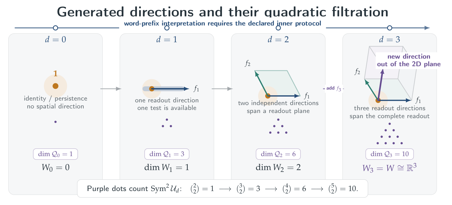
Problem 2 (Operator realization of the quadratic filtration). Construct a positive-frequency invariant graded sector \(K=\bigoplus_{d=0}^{3}K_d\), bounded or precisely domain-controlled operators \(T_{\mathrm i},T_{\mathrm o}\) satisfying the rank-one commutator-growth hypotheses of Proposition 16, and natural unitary identifications

that intertwine the filtration maps. Such a result would provide an operator origin for the ladder \((1,2,3,4)\) while leaving the separate free symmetric, exterior, and reconstruction laws explicit.

This separation is visualized in Figure 3: a complete flag presents subspaces of ranks \(0,1,2,3\) inside \(W\), the symmetric-closure dimensions are \(1,3,6,10\), and the scalar identity channel remains nonspatial. Theorem 4 supplies one ordered protocol generating such a flag. The figure also applies to arbitrary supplied flags; a displayed inclusion alone is not an evolution law.

8. Free Alternating Branches and Global Depth-Homogeneous Reconstruction

8.1. The Positive-Degree Alternating Branch Object

For the complete flag above, define the innovation space

Principle 15 (Oriented alternating innovation law). Independent innovations compose multilinearly. Repetition of the same innovation produces no new branch, and exchange of two innovations reverses branch orientation. No additional quotient relation is imposed before record closure. Multilinearity represents dependence on independently supplied innovation vectors; the vanishing of repeated vectors and orientation reversal select the alternating exchange rule. This is the operational meaning assigned to innovations in this signature, not a consequence of the readout dimension or the spin-statistics theorem. A signless Boolean support law would be a different construction; the exterior receiver is selected only by this oriented alternating law.

Definition 10 (Positive-degree alternating receiver). A positive-degree alternating receiver for a complex vector space \(I\) is a positively graded, generally nonunital, associative \(\mathbb{C}_{\mathrm{ph}}\)-algebra

together with a linear map \(j:I\to A_1\) satisfying \(j(v)^2=0\) for every \(v\in I\). For fixed \(I\), morphisms are graded nonunital algebra maps \(f:A^+\to A^{\prime +}\) satisfying \(f\circ j=j’\). Denote this receiver category by \(\mathsf{AltRec}^{+}_{\mathbb{C}_{\mathrm{ph}}}(I)\).

Theorem 11 (Positive-degree exterior universal property). The pair

is initial among positive-degree alternating receivers for \(I\).

Proof. Let \(T^+(I)=\bigoplus_{k\geq1}I^{\otimes k}\) be the positive-degree tensor algebra. It is free among positively graded nonunital associative algebras receiving a linear map from \(I\). Quotienting by the two-sided ideal generated by \(v\otimes v\) imposes exactly the alternating relation. Over \(\mathbb{C}_{\mathrm{ph}}\), polarization of \((u+v)^2=0\) gives \(uv=-vu\). The quotient is \(\Lambda^{\geq1}I\), and every alternating receiver admits a unique induced graded nonunital algebra map. \(\square\)

Definition 11 (Free exterior branch sectors). For \(d=0,1,2,3\), put

and let

be the canonical degree-one generator map. Choosing the initial positive-degree receiver rather than a further quotient is called the free exterior-completion rule. Give every exterior power its standard induced Hermitian form and \(\mathfrak B_d\) the orthogonal direct-sum form.

Corollary 5 (Exterior branch dimensions). For every \(d\in\{0,1,2,3\}\),

so the branch-dimension ladder is \((0,1,3,7)\). In an adapted oriented basis, exterior monomials are indexed by nonempty supports, while odd permutations reverse orientation.

Figure 4 keeps the flag ranks and exterior-branch ranks visible together. Its arrows denote inclusions; when the flag is generated by the word protocol, the temporal interpretation belongs to that separately specified protocol.

8.2. Symmetric and Exterior Receivers as Quantum-Statistical Templates

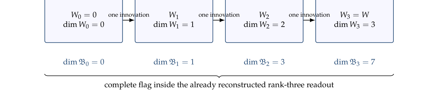
In conventional many-particle quantum theory, symmetric tensor powers organize bosonic exchange sectors and exterior powers organize fermionic exchange sectors. Schematically, for a one-particle Hilbert space \(\mathcal H_1\),

see, for example, [27,28]. This standard structure explains a useful mathematical connection. The receiver \(\mathcal Q_d=\operatorname{Sym}^2\mathcal U_d\) retains unordered quadratic pair data, while \(\mathfrak B_d=\Lambda^{\geq1}\mathcal I_d\) retains oriented alternating combinations and removes repeated innovations. They therefore provide symmetry types compatible with the two basic exchange grammars of quantum theory.

Here this is a correspondence between symmetry types. The spaces \(\mathcal U_d\) and \(\mathcal I_d\) have not been proved to be physical one-particle Hilbert spaces; the exterior grading records construction degree rather than particle number or super parity; and Proposition 18 explicitly uses the ordinary tensor symmetry after totalization. No Fock vacuum, creation and annihilation operators, canonical commutation or anticommutation relations, spin-statistics theorem, Hamiltonian, locality condition, or particle species is constructed. In particular, the finite receiver \(\mathfrak R_3\) is not being renamed a truncated Fock space.

The controlled conclusion is that the reconstruction contains a pre-statistical grammar: symmetric pairing and alternating exclusion are already separated at the carrier level. A later quantum realization may map these universal receivers into bosonic, fermionic, or more general graded sectors, but that map and its dynamics must be derived independently and must preserve the distinctions between sources, records, and phase roles.

Definition 12 (Finite closure linearization). Let \(\mathsf{AltAlg}^{+,\mathrm{fd}}_{\mathbb{C}_{\mathrm{ph}}}\) be the category of positively graded, nonunital, associative \(\mathbb{C}_{\mathrm{ph}}\)-algebras having only finitely many nonzero finite-dimensional graded pieces; its morphisms are degree-preserving algebra maps. Let \(\mathsf{GrVect}^{\geq 0,\mathrm{fd}}_{\mathbb{C}_{\mathrm{ph}}}\) be the category of finite-dimensional nonnegatively graded \(\mathbb{C}_{\mathrm{ph}}\)-vector spaces and degree-preserving linear maps, equipped with the ordinary tensor-product grading and ordinary flip symmetry. Its tensor unit is \(\mathbb{C}_{\mathrm{ph}}\) concentrated in degree zero. Let \(\mathsf{Vect}^{\mathrm{fd}}_{\mathbb{C}_{\mathrm{ph}}}\) be the category of finite-dimensional \(\mathbb{C}_{\mathrm{ph}}\)-vector spaces and linear maps. Define

by forgetting multiplication and adjoining the zero degree-zero component, and define totalization

The closure-linearization functor is

For the finite exterior branch algebra \(\mathfrak B_d\), put

where \(\mathcal I_d\) is regarded as concentrated in degree one. We equip \(\overline{\mathfrak B}_d\) with the orthogonal direct-sum Hermitian form induced from the standard forms on the exterior powers. This Hermitian structure belongs to the specified exterior branch objects; it is not part of the abstract forgetful functor. Forgetting multiplication and forgetting grading are separate operations. Totalization is an explicit choice of output signature, not a necessary condition for a common scalar phase.

Proposition 17 (Multiplication obstruction and grading-compatible coherent phase). On \(\mathfrak B_d=\Lambda^{\geq1}\mathcal I_d\), the polynomial phase \(\rho_z(x)=z^kx\) for \(x\in\Lambda^k\mathcal I_d\) preserves both grading and multiplication. The common weight-one action

is a degree-preserving unitary circle action on \(\mathsf U_{\mathrm{gr}}(\mathfrak B_d)\). If some product \(xy\) is nonzero, \(\sigma_z\) is not an algebra automorphism for \(z\neq1\). Consequently, retaining the full coherent circle requires omitting branch multiplication from the preserved structure, but does not require deleting construction degree.

Proof. For homogeneous \(x\) and \(y\) of degrees \(k\) and \(\ell\), \(\rho_z(xy)=z^{k+\ell}xy=\rho_z(x)\rho_z(y)\). Scalar multiplication preserves each homogeneous subspace and satisfies \(\sigma_z\sigma_w=\sigma_{zw}\), so \(\sigma\) is a graded unitary action. If \(xy\neq0\), then

The obstruction occurs for \(d\geq2\); at \(d=1\) the positive-degree exterior algebra has zero multiplication. Construction degree and representation weight are therefore distinct: a component can retain exterior degree \(k\) while carrying coherent circle weight one. \(\square\)

8.3. Reconstruction-Level Linearization, Depth Homogeneity, and Free Completion

Definition 13 (Pre-closure graded diagrams and their framed fiber). A height-three pre-closure graded reconstruction diagram is a tuple

with \(Q^{\mathrm{gr}},I_d,X_d\in\mathsf{GrVect}^{\geq 0,\mathrm{fd}}_{\mathbb{C}_{\mathrm{ph}}}\), \(X_0=0\), each \(I_d\) concentrated in degree one, \(B_d\in\mathsf{AltAlg}^{+,\mathrm{fd}}_{\mathbb{C}_{\mathrm{ph}}}\), and a degree-preserving map

whose image lies in degree one and for which \((B_d,\iota_d)\) is a positive-degree alternating receiver of \(I_d\). The structure maps are degree-preserving maps

A morphism is a tuple

consisting of graded linear maps \(a_Q,a_{I_d},a_{X_d}\) and graded algebra maps \(a_{B_d}\) satisfying

Denote this category by \(\mathsf{Rec}^{\mathrm{gr}}\). Write \(\mathcal Q\langle2\rangle\) for \(\mathcal Q\) concentrated in polynomial degree \(2\). The framed fiber

has fixed sources \(Q^{\mathrm{gr}}=\mathcal Q\langle2\rangle\), \(I_d=\mathcal I_d\langle1\rangle\), \(B_d=\mathfrak B_d\), and \(\iota_d\) equal to the canonical exterior generators; all source components of a framed morphism are identities.

Definition 14 (Linearized diagrams and reconstruction-level linearization). A height-three linearized reconstruction diagram is a tuple

with \(Q,I_d,\overline B_d,X_d\in\mathsf{Vect}^{\mathrm{fd}}_{\mathbb{C}_{\mathrm{ph}}}\), \(X_0=0\), and linear maps

Morphisms are tuples on all source and receiver spaces preserving \(\overline\iota_d\), \(p_d\), and \(j_d\). Denote this category by \(\mathsf{Rec}^{\mathrm{lin}}\). There is also an intermediate category \(\mathsf{Rec}^{\mathrm{grlin}}\) defined by the same diagram, with all objects nonnegatively graded and all maps degree-preserving. Its branch objects are graded vector spaces, without multiplication. Thus the two forgetting operations factor as

Here \(F_{\mathrm{alg}}\) applies \(\mathsf U_{\mathrm{gr}}\) to branch objects and their maps; \(\mathsf{Tot}_{\mathrm{rec}}\) totalizes every object and map. The framed fiber of \(\mathsf{Rec}^{\mathrm{lin}}\)

has fixed sources \(Q=\mathcal Q\), \(I_d=\mathcal I_d\), \(\overline B_d=\overline{\mathfrak B}_d\), and \(\overline\iota_d=\mathsf{Tot}(\iota_d)\), with all source components of every morphism equal to the identity.

Define

by

by sending \(\iota_d\) to \(\mathsf{Tot}(\iota_d)\), and by totalizing every propagation, branch-incidence, and morphism component. The canonical finite-grading identification

makes the propagation maps well defined. Thus \(\mathsf{Cl}_{\mathrm{rec}}\) omits multiplication and construction-degree labels from the diagram signature while retaining the innovation generators and all displayed incidence maps. It restricts to a functor between the two framed fibers displayed above. If an action is already specified, the functor transports its linear operators unchanged; it does not erase or replace their representation weights. In particular, forgetting the grading of an object must not be confused with forgetting a specified polynomial circle action on that object.

On the selected diagram \(F_{\mathrm{alg}}(\mathfrak D^{\mathrm{pre}}_{\mathfrak R})\) of Definition 15, identity on \(\mathcal Q\langle2\rangle\) and uniform weight one on innovations, branches, and receivers preserve all degrees and all displayed arrows: \(z\iota_d=\iota_d z\), \(zp_d=p_d(\operatorname{Id}\otimes z)\), and \(zj_d=j_dz\). This coherent action already exists in \(\mathsf{Rec}^{\mathrm{grlin}}\), although it does not lift through \(F_{\mathrm{alg}}\) to branch algebra automorphisms. Totalization is therefore an additional modeling rule.

Proposition 18 (Well-definedness of closure and reconstruction linearization). The assignments \(\mathsf U_{\mathrm{gr}}\), \(\mathsf{Tot}\), \(\mathsf{Cl}_{\mathrm{lin}}=\mathsf{Tot}\circ\mathsf U_{\mathrm{gr}}\), \(F_{\mathrm{alg}}\), \(\mathsf{Tot}_{\mathrm{rec}}\), and \(\mathsf{Cl}_{\mathrm{rec}}\) are functors. On finite nonnegatively graded vector spaces, totalization is additive and is strong symmetric monoidal for the ordinary tensor symmetry:

The grading records construction degree rather than super parity, so no Koszul sign is inserted in the symmetry. Consequently, totalizing a degree-preserving propagation or generator map produces a well-defined linear map, and all generator, incidence, identity, and composition relations are preserved. For the selected finite exterior objects, the orthogonal direct-sum Hermitian forms make totalized unitary graded maps unitary.

Proof. The functor \(\mathsf U_{\mathrm{gr}}\) forgets multiplication while retaining the graded vector space. Its image has zero degree-zero component, so it lies in the nonnegative graded category. Since every object of \(\mathsf{GrVect}^{\geq 0,\mathrm{fd}}_{\mathbb{C}_{\mathrm{ph}}}\) has only finitely many nonzero finite-dimensional pieces, \(\mathsf{Tot}\) is a finite direct sum. The tensor comparison sends a homogeneous tensor in \(A_i\otimes B_j\) to the same tensor in the tensor product of the total spaces; the direct-sum decomposition by \(i+j\) makes this map natural and invertible, while the degree-zero unit is carried to the ordinary tensor unit. The direct-sum comparison is immediate. Applying these maps objectwise preserves the generator and incidence equations, proving functoriality of \(\mathsf{Cl}_{\mathrm{rec}}\). The metric statement follows from the standard tensor-product and orthogonal direct-sum Hermitian forms. \(\square\)

Remark 10 (Completion versus observation). A fuller categorical reconstruction theory should distinguish completion from observation. One natural architecture is a reflective subcategory \(\mathsf{Comp}\hookrightarrow\mathsf{State}\) with reflector \(K\dashv J\), so that \(JK\) is an idempotent completion monad, followed by an observation functor \(P:\mathsf{Comp}\to\mathsf{Obs}\) that forgets hidden chronology or latent construction data. This separation is useful because completion may be idempotent while observation remains many-to-one. The functor \(\mathsf{Cl}_{\mathrm{rec}}\) defined above models only the finite algebraic forgetting/totalization of already specified reconstruction data; it is not asserted to be the physical reflector \(K\), the observation functor \(P\), or their composite. In particular, the present paper does not identify categorical completion with deletion of grading: completion and observational forgetting are distinct operations whose coincidence would require a separate theorem. Here the word “monad” in the categorical sense is a technical term and is not the ontic Monad of SMM. Standard categorical background is given in [29,30].

Problem 3 (Reflective realization of reconstruction closure). Construct categories \(\mathsf{State}\), \(\mathsf{Comp}\), and \(\mathsf{Obs}\), a fully faithful inclusion \(J:\mathsf{Comp}\hookrightarrow\mathsf{State}\) with left adjoint \(K\), an observation functor \(P:\mathsf{Comp}\to\mathsf{Obs}\), and realization functors

together with a natural isomorphism

If a recurrence or history monad \(T_{\mathrm{adm}}\) is present, require a Beck distributive law

so that generation and completion are compatible without being identified. Such a theorem would turn the present formal boundary linearization into a derived physical completion-and-observation process.

Principle 16 (Global depth-homogeneous completion and independent adjoining). After the full rank-three readout and its quadratic closure \(\mathcal Q\) have been constructed, every filtration depth uses the same propagation endofunctor

Previously admitted content and the newly available branch source enter independently by coproduct. Before closure this is a coproduct of graded spaces; after applying \(\mathsf{Cl}_{\mathrm{rec}}\) it is a direct sum of complex vector spaces. No additional relation is imposed. Stage-sensitive completion by \(\mathcal Q_d\) or \(\mathcal G_d\) is a different model and is audited in §Appendix A.

Why One Stage per Flag Level, and Why the Full Propagator?

The chosen complete flag has three successive one-dimensional quotients, so assigning one adjoining operation to each strict inclusion gives height three. This is the specified maximal-refinement convention; a partial flag, repeated stages, or a different termination rule would define another signature. The full \(\mathcal Q=\operatorname{Sym}^2(\mathbb{C}_{\mathrm{ph}}\otimes(\mathbb{R}1\oplus W))\) is used at every stage because the propagation operation is required here to be depth independent on the already available full carrier. Such stationarity lets contributions from different depths be compared through powers of one operator-valued source. It is a motivation for studying a uniform free construction, not a proof that a physical process uses that propagator. If only stage-local pair data are available, \(\mathcal Q_d\) is a natural alternative and gives a different receiver. No independent physical selection principle for height three or full-\(\mathcal Q\) propagation is established.

Remark 11 (Global filtration, not yet chronological dynamics). The acquisition depth in Theorem 4 and the receiver depth here have different roles. First the word protocol generates and completes \(W\) and records its prefix flag; then \(\mathcal Q=\mathcal Q_3\) is formed on that complete carrier and the homogeneous receiver recursion is evaluated along the retained flag. Thus use of the full \(\mathcal Q\) at early receiver depths does not assert that unavailable future directions participate in live acquisition. A strictly stage-local propagation rule would instead use \(\mathcal Q_d\) and has a different count, as shown in Table 6. Neither the word protocol nor outer transport selects the homogeneous rule.

Definition 15 (Free pre-closure and linearized reconstructions). Define the receiver components \(\mathfrak R^{\mathrm{pre}}_0=0\) and

with canonical graded summand inclusions and the canonical receiver triples \((\mathcal I_d\langle1\rangle,\mathfrak B_d,\iota_d)\), and denote the resulting full diagram by \(\mathfrak D^{\mathrm{pre}}_{\mathfrak R}\). Set

and denote its receiver components by \(\mathfrak R_d\). Explicitly,

The selected finite vector spaces carry their standard induced Hermitian forms.

Theorem 12 (Initiality before and after linearization). The pre-closure diagram \(\mathfrak D^{\mathrm{pre}}_{\mathfrak R}\) is initial in \(\mathsf{Rec}^{\mathrm{gr,fr}}_{\mathcal Q\langle2\rangle,\mathcal I,\mathfrak B}\), and its image \(\mathfrak D^{\mathrm{lin}}_{\mathfrak R}\) is initial in \(\mathsf{Rec}^{\mathrm{lin,fr}}_{\mathcal Q,\mathcal I,\overline{\mathfrak B}}\).

Proof. In either category set the map at depth zero equal to the zero map. If the map at depth \(d-1\) has been defined, the direct-sum universal property gives a unique depth-\(d\) map whose first summand is the target propagation map composed with \(\operatorname{Id}_{\mathcal Q}\otimes f_{d-1}\) and whose second summand is the target branch map. In the graded category every map is degree-preserving; after totalization the same argument applies in the linear category. \(\square\)

Proposition 19 (Framed rigidity and the output-forgetful functor). The initial linearized reconstruction has only the identity endomorphism:

In particular, a nontrivial scalar multiple of the receivers is not a framed endomorphism. Let

be the depth-three output-forgetful functor. Scalar phases on \(\mathsf{Out}_3(\mathfrak R)\) therefore belong either to the forgotten output space or to an enlarged diagram automorphism that also acts on source objects; they do not belong to the framed endomorphism monoid.

Proof. An initial object has a unique endomorphism. Explicitly, the relation \(f_1j_1=j_1\) with nonzero branch inclusion forces a uniform scalar \(f_1=z\operatorname{Id}\) to have \(z=1\). \(\square\)

Corollary 6 (Closed form of the depth-three receiver). There are natural isomorphisms

The exponent \(3-d\) is the number of remaining homogeneous completion factors assigned to the contribution entering at filtration depth \(d\).

Proof. Expand Eq. (37) successively. The second isomorphism uses the symmetry of the tensor category of complex vector spaces. \(\square\)

Proposition 20 (Flag-groupoid functoriality and unitary transport). Let \(\mathsf{Flag}^+(W)\) be the action groupoid whose objects are complete flags in the oriented Euclidean space \(W\), with the proper subspaces \(W_1\) and \(W_2\) unoriented, and whose morphisms \(F\to F’\) are elements \(g\in SO(W)\) satisfying \(gF=F’\). The superscript \(+\) refers only to the orientation of the ambient space. The assignments

define a functor to the corresponding reconstruction diagram categories. After the selected source and receiver spaces are equipped with their standard Hermitian forms, every flag-groupoid morphism is represented by compatible unitary maps. For every flag the stabilizer is

in an adapted oriented orthonormal basis. Thus different morphisms between the same flags can induce different transports; no identification independent of the chosen morphism is asserted.

Proof. An isometry preserving the flag preserves each of the three orthogonal lines \(W_1\), \(W_2\cap W_1^\perp\), and \(W_2^\perp\). It acts on them by signs whose product is \(+1\), proving the stabilizer formula. Every nonidentity element of this stabilizer acts nontrivially on \(\mathcal I_3\), so its action on the full source diagram is nontrivial. A morphism \(g:F\to F’\) restricts to isometries \(W_d\to W’_d\). Scalar extension gives unitary maps on \(\mathcal I_d\) and \(\mathcal U_d\) and intertwines the canonical generator maps \(\iota_d\). Symmetric powers, exterior powers, totalization, tensor products, and orthogonal direct sums preserve the relevant maps and composition. The two recursions then determine compatible maps on \(\mathfrak R^{\mathrm{pre}}_d\) and \(\mathfrak R_d\), which are unitary for the selected induced forms. \(\square\)

Proposition 21 (Dimension recursion and closed formula). Let \(m:=\dim_{\mathbb{C}_{\mathrm{ph}}}\mathcal Q\) and \(r_d(m):=\dim_{\mathbb{C}_{\mathrm{ph}}}\mathfrak R_d\). Then

and

For \(m\neq1,2\),

At \(m=1,2\),

For \(m=10\), the dimension sequence is

Proof. Taking dimensions in Eq. (37) gives the recurrence. Iteration gives the finite sum. Splitting it into two geometric sums gives the closed form; the exceptional values follow directly or by limits. \(\square\)

Theorem 13 (Depth-three reconstruction dimension). The free height-three reconstruction has

Equivalently, its dimension polynomial is

Proof. Apply Theorem 10, Theorem 5, and Corollary 6; totalization preserves the dimensions of the branch sectors, and dimension is multiplicative under tensor product. \(\square\)

Remark 12 (Semiring decategorification). Let \(K_0^+(\mathsf{Vect}^{\mathrm{fd}}_{\mathbb{C}_{\mathrm{ph}}})\) denote the commutative semiring of isomorphism classes of finite-dimensional complex vector spaces under direct sum and tensor product. Dimension is the semiring morphism

Applying it to the recursive object identity

gives

Thus \(N_3(t)=t^2+3t+7\) is the decategorified dimension polynomial of the displayed reconstruction object, not the primitive object from which that object is inferred. This relates the object-level construction to its dimension polynomial; compare standard species and polynomial-functor methods in [31].

The three direct-sum contributions are displayed in Figure 5.

Theorem 14 (Universal characterization within the declared reconstruction signature). Within the reconstruction signature specified below, and up to unique natural isomorphism, the assignment

is determined by the following laws:

1. (C1) reconstruction uses the unital envelope \(E_d=\mathbb{R}\mathbf1\oplus W_d\);

2. (C2) quadratic closure is the free receiver of symmetric bilinear pair data;

3. (C3) nonempty branch composition is the free positive-degree receiver of alternating innovation data;

4. (C4) pre-closure construction degree is additive, with \(\mathcal Q\) concentrated in degree \(2\) and \(\Lambda^k\mathcal I_d\) in degree \(k\);

5. (C5) the same propagation endofunctor \(\mathcal Q\langle2\rangle\otimes-\) is used at every filtration depth;

6. (C6) propagated content and newly entering branch content are adjoined by coproduct, with no further relations;

7. (C7) boundary linearization first forgets branch multiplication and then totalizes, \(\mathsf{Cl}_{\mathrm{rec}}=\mathsf{Tot}_{\mathrm{rec}}\circ F_{\mathrm{alg}}\); deleting degree is part of this law, not forced by coherent phase.

These laws determine

the graded recursion for \(\mathfrak R^{\mathrm{pre}}_d\), and its totalized linear recursion Eq. (37).

Proof. Laws (C1)–(C2) determine \(\mathcal Q_d\) by Proposition 14; law (C3) determines \(\mathfrak B_d\) by Theorem 11. Law (C4) fixes the pre-closure grading. Laws (C5)–(C6) determine \(\mathfrak R^{\mathrm{pre}}_d\) inductively as the graded coproduct

Law (C7) then determines \(\overline{\mathfrak B}_d\), the transported generator \(\overline\iota_d\), and \(\mathfrak R_d\) by totalization. The universal properties at each stage yield uniqueness only within this declared signature. \(\square\)

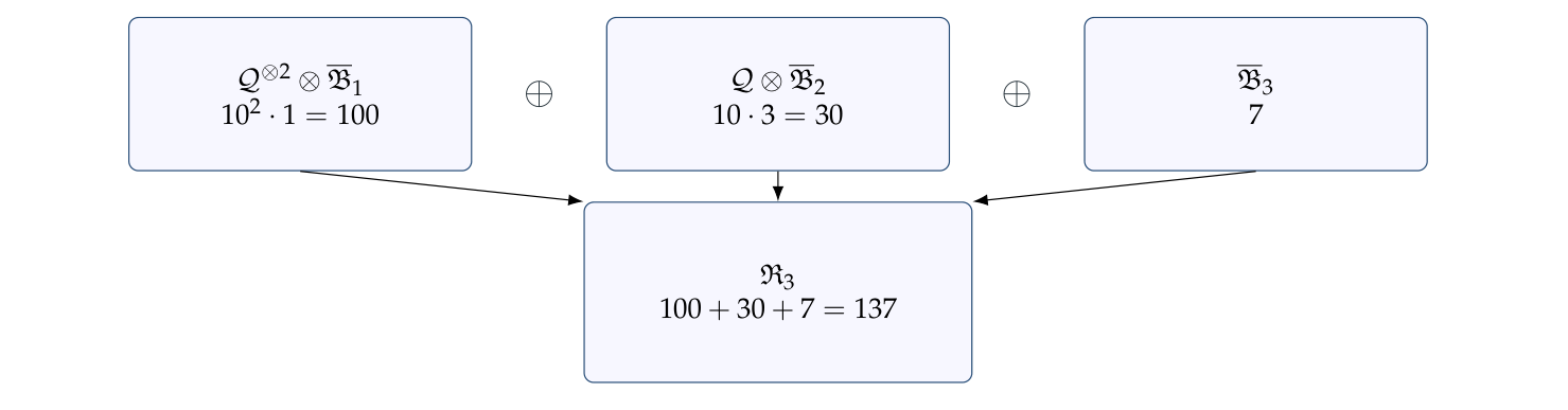
Remark 13 (Status of the free laws). The theorem proves uniqueness within the declared signature, not uniqueness among all mathematically natural reconstruction theories. The numbers \(10\) and \(137\) are dimensions of displayed objects, but the laws in Theorem 14 remain explicit constitutive rules. A physical theory must derive why its relevant sector realizes these free objects rather than quotients, stage-dependent propagators, or different polynomial functors.

8.4. Relations in Arbitrary Receivers: A Sharp Rank and Phase Comparison

Initiality gives more than a preferred dimension: it controls the loss of independent data in every receiver with the same sources and propagation signature. The following statement concerns linear relations; it assumes no physical realization.

Theorem 15 (Generated receivers and the rank defect). Let \(X\) be an arbitrary object of \(\mathsf{Rec}^{\mathrm{lin,fr}}_{\mathcal Q,\mathcal I,\overline{\mathfrak B}}\). Define its generated subsystem by

and let

Put \(s_d=\dim_{\mathbb{C}_{\mathrm{ph}}}X^{\mathrm{gen}}_d\) and \(\kappa_d=\dim_{\mathbb{C}_{\mathrm{ph}}}\ker A_d\). The unique initial evaluation \(e_d:\mathfrak R_d\to X^{\mathrm{gen}}_d\) is surjective at every depth, and

In particular \(0\leq s_3\leq137\). Equality \(s_3=137\) holds if and only if every \(A_d\) is injective, equivalently if and only if all the evaluations \(e_d\) are isomorphisms.

Proof. Restricting propagation to the displayed subspaces makes \(X^{\mathrm{gen}}\) a receiver with the same framed sources. By Theorem 12, its unique evaluation is given recursively by

The map \(A_d\) is surjective by the definition of \(X^{\mathrm{gen}}_d\). Induction, and preservation of surjections by tensor products of vector spaces, show that \(e_d\) is surjective. Rank–nullity, \(\dim\mathcal Q=10\), and \(\dim\overline{\mathfrak B}_d=2^d-1\) give the recurrence. Its first three steps are

All defects are nonnegative. Thus \(s_3=137\) exactly when they all vanish. In that case every \(A_d\) is an isomorphism, and the recursive formula proves that every \(e_d\) is an isomorphism. Conversely, if the evaluations are isomorphisms, the same formula makes every \(A_d\) an isomorphism. \(\square\)

Corollary 7 (Scalar phase survives arbitrary linear relations). The coherent action, identity on \(\mathcal Q\) and weight one on innovations, branches, and generated receivers, descends through every evaluation above. Its terminal determinant character is \(z\mapsto z^{s_3}\), whose kernel is \(\mu_{s_3}\) when \(s_3>0\) and the full circle when \(s_3=0\). These are determinant kernels; selecting them as closure phases remains an additional rule.

Proof. Both summands in the domain of \(A_d\) carry the scalar action \(z\operatorname{Id}\), so every linear kernel is invariant and \(A_d\) intertwines the induced action with \(z\operatorname{Id}\) on its image. The same applies to \(e_d\). All linear incidence and propagation maps therefore intertwine the simultaneous actions; the innovation incidence map also does so. Scalar multiplication on a space of dimension \(s_3\) has determinant \(z^{s_3}\), with determinant \(1\) on the zero space. The action is unitary for any Hermitian forms. As in Definition 18, it acts on the sources too and is an unframed diagram automorphism, not a nonidentity framed endomorphism. \(\square\)

The coefficients \(100,10,1\) quantify the terminal effect of independent relations first introduced at successive depths: a relation propagates through two, one, or zero remaining copies of \(\mathcal Q\). These defects are measured after earlier relations have already been imposed, so inherited relations are not counted twice. Thus \(137\) is the sharp generated-rank bound for this signature, with equality characterizing absence of linear relations.

Remark 14 (Example: a relation separating the two phase actions). In \(\mathfrak R_2=(\mathcal Q\otimes\overline{\mathfrak B}_1)\oplus\overline{\mathfrak B}_2\), choose nonzero \(v\) in the first summand and nonzero \(w\in\Lambda^1\mathcal I_2\) in the second. Put \(X_1=\mathfrak R_1\), \(X_2=\mathfrak R_2/\langle v+w\rangle\), and \(X_3=(\mathcal Q\otimes X_2)\oplus\overline{\mathfrak B}_3\), with the induced source and propagation maps. Then \((\kappa_1,\kappa_2,\kappa_3)=(0,1,0)\) and \(\dim X_3=127\). The coherent action descends by the corollary. The transported polynomial action does not: it has weights \(3\) on \(v\) and \(1\) on \(w\), so the relation line is not invariant under the whole circle. In general a specified action descends through an evaluation precisely when its kernel is invariant. This distinguishes a consequence of linear scalar coherence from a consequence of merely forgetting construction-degree labels.

8.5. A Representation Obstruction to Removing the Flag

Flag-groupoid covariance does not imply that the output is the restriction of a single representation of all rotations on one fixed vector space. The following calculation distinguishes these statements for the declared reconstruction. Throughout, a flag consists of an unoriented line in an unoriented plane inside the oriented Euclidean space \(W\). Rotations act on \(W\) and its reconstruction objects; they are not required to fix the separately supplied distinguished quaternionic phases \(j_1,j_2\).

Theorem 16 (Stabilizer character and failure of representation extension). Let \(G=SO(W)\), let \(F=(W_1\subset W_2\subset W)\), and choose an oriented orthonormal adapted basis \((e_1,e_2,e_3)\). Its flag stabilizer is

Write \(\chi_a(k)=\varepsilon_a\) and \(\mathbf1\) for the trivial character. For the natural \(K\)-action on the depth-three receiver,

This \(K\)-representation does not extend to a complex representation of \(G\). Consequently, the equivariant receiver bundle over the flag space \(G/K\) has no \(G\)-equivariant trivialization \((G/K)\times V\) in which \(G\) acts on the fixed fiber \(V\) through a single representation of \(G\).

Proof. A rotation preserving the line and plane also preserves their orthogonal successive complements. It is therefore diagonal in the adapted basis, with the displayed signs and determinant condition. Conversely, every such diagonal map preserves the flag. The four characters of \(K\) are \(\mathbf1,\chi_1,\chi_2,\chi_3\), with \(\chi_a^2=\mathbf1\) and \(\chi_1\chi_2=\chi_3\). Using direct sums additively in the representation ring,

The four diagonal symmetric squares have trivial character; the six mixed pairs contribute two copies of each nontrivial character. The exterior branches have characters

Here totalization changes neither the underlying \(K\)-action nor its character. Multiplying these expressions in the representation ring gives

Adding \(\overline{\mathfrak B}_3\) proves Eq. (41); the multiplicities sum to \(137\).

Let \(k_a\) be the half-turn about the \(e_a\)-axis. These three elements of \(K\) are conjugate in \(G\). The character in Eq. (41) has respective values

Since the character of any \(G\)-representation is constant on \(G\)-conjugacy classes, an extension is impossible.

For completeness, write \(\tau:K\to U(\mathfrak R_3(F))\) for the stabilizer action. The transported family is the associated equivariant vector bundle \(G\times_K\mathfrak R_3(F)\to G/K\), with \([gk,v]=[g,\tau(k)v]\). An equivariant isomorphism to \((G/K)\times V\), with diagonal action induced by a representation \(\rho:G\to GL(V)\), restricts at \(eK\) to an invertible intertwiner \(A\tau(k)=\rho(k)A\). Conversely, such an intertwiner defines the equivariant isomorphism

Thus this type of equivariant trivialization exists exactly when \(\tau\) extends, which it does not. \(\square\)

Remark 15 (Scope and dependence on the orientation convention). The receiver family is a well-defined \(G\)-equivariant vector bundle over \(G/K\); the theorem does not obstruct that construction and makes no assertion about ordinary, nonequivariant trivializations. It obstructs removing the flag while retaining its specified rotation transport on one fixed representation space. This supplies information not contained in the common dimension: the first flag line remains detectable by the unequal half-turn traces.

If the line and plane are separately oriented as well, preserving those orientations forces \(\varepsilon_1=\varepsilon_2=\varepsilon_3=1\), so the stabilizer is trivial. The stated character obstruction then disappears; it cannot be transferred unchanged to that different flag convention. Neither convention supplies a physical rule selecting a flag or identifying its filtration with time.

8.6. A Natural Nine-Dimensional Comparison and a Rank-128 Quotient

The height-two receiver formed with the stage-local quadratic space \(\mathcal Q_2\) gives a comparison with the homogeneous height-three construction. It does not replace its intermediate receiver: throughout the original recursion, \(\mathfrak R_2=(\mathcal Q\otimes\overline{\mathfrak B}_1)\oplus\overline{\mathfrak B}_2\) has dimension \(13\). Instead define the separate comparison object

Thus \(\dim S_2=N_2(6)\) for \(N_2(t)=t+3\), whereas \(\dim\mathfrak R_2=N_2(10)\). The following exact sequence gives \(N_3(10)-N_2(6)=128\) an object-level meaning.

Theorem 17 (Natural terminal quotient and its symmetries). For a flag \(F\), let \(u:\mathcal Q_2\hookrightarrow\mathcal Q\), \(v:\overline{\mathfrak B}_1\hookrightarrow\overline{\mathfrak B}_2\), and \(w:\overline{\mathfrak B}_2\hookrightarrow\overline{\mathfrak B}_3\) be the inclusions induced by its symmetric and exterior powers. Relative to the ordered decomposition in Eq. (38), the map

is injective. Its cokernel \(E_{128}(F)\) gives a natural exact sequence over the flag groupoid of Proposition 20,

The coherent and polynomial actions of Definition 19 both descend to this quotient, with determinant characters

For the stabilizer and character convention of Theorem 16,

Its three stabilizer half-turn traces are \(0,-4,-4\), so this \(K\)-representation likewise does not extend to an \(SO(W)\) representation on one fixed fiber.

Proof. Symmetric and exterior powers preserve inclusions of vector spaces, and tensor products preserve injections over \(\mathbb{C}_{\mathrm{ph}}\). The two components of \(\iota_F\) lie in distinct direct summands, so their injectivity proves that of \(\iota_F\). Their dimensions are \(6\) and \(3\), respectively. Consequently the quotient decomposes naturally as

with dimensions \(100\), \(30-6\), and \(7-3\). Every flag-groupoid morphism intertwines \(u,v,w\), hence \(\iota_F\), and therefore induces a map on the cokernel. Composition is preserved. Equipping the cokernel with the quotient Hermitian form makes this transport unitary.

The coherent action is scalar of weight one on the entire receiver, so preserves the image and gives determinant exponent \(128\) on the quotient. For the polynomial action, the removed six-dimensional sector has weight \(3\), while the removed copy of \(\overline{\mathfrak B}_2\) has weights \(1,1,2\). The image is invariant and has determinant exponent \(6\cdot3+2\cdot1+1\cdot2=22\). Subtracting from the ambient exponent \(612\) in Proposition 23 gives \(590\).

Finally \(\mathcal U_2|_K=\mathbf1+\chi_1+\chi_2\) gives

Subtracting from Eq. (41) proves Eq. (46). Its unequal traces on the three half-turns, which are conjugate in \(SO(W)\), obstruct extension by the same character argument as in Theorem 16. This still permits the associated equivariant bundle over \(SO(W)/K\). \(\square\)

Corollary 8 (Rank \(128\) requires a terminal defect). In the generated-receiver class of Theorem 15, terminal dimension \(128\) forces \((\kappa_1,\kappa_2,\kappa_3)=(0,0,9)\). The quotient above realizes these defects by keeping \(X_1=\mathfrak R_1\), \(X_2=\mathfrak R_2\), and setting \(X_3=E_{128}\), with terminal propagation and branch maps followed by the quotient map.

Proof. The rank formula gives \(100\kappa_1+10\kappa_2+\kappa_3=9\). Nonnegative integrality forces the stated values. For the displayed realization, the first two adjoining maps are isomorphisms and the third is the quotient by the nine-dimensional image of \(\iota_F\). \(\square\)

Remark 16 (Naturality does not select a unique subtraction). There is another natural injection using the distinguished invariant vector \(q_0=\mathbf1\odot\mathbf1\in\mathcal Q\):

Its image again has dimension \(9\) and the same \(K\)-character, so its quotient has dimension \(128\), coherent determinant exponent \(128\), and the same rotational obstruction. For polynomial phase the extra \(q_0\) has weight \(2\): the source must be shifted by two construction degrees to make this injection equivariant. Its invariant image then has determinant exponent \(22+2\cdot9=40\), leaving exponent \(612-40=572\) on the quotient. Thus the two natural embeddings have different polynomial phase data. A physical rule selecting a removed sector requires more than its dimension, flag covariance, or coherent determinant. Neither quotient alone identifies its removed sector with vacuum polarization or supplies an electromagnetic coupling.

The exact sequences establish conditional reconstruction comparisons, not an energy limit. Their undressed vacuum-sector interpretation is defined in Definition 16. Even for the first quotient, interpreting the kernel of its coherent determinant as a closure rule is additional: under that rule the kernel is \(\boldsymbol\mu_{128}^{\mathrm{out}}\), while the corresponding polynomial kernel is \(\boldsymbol\mu_{590}^{\mathrm H}\). Identifying a normalized closure phase with a measured, scale-dependent coupling requires the separate physical matching conditions discussed in §12.

8.7. Inner Dimensional Acquisition and Conditional Uniqueness of the Rank Pair

The generated dimensions and the receiver dimensions belong to successive constructions. The word protocol first acquires a complete three-dimensional readout and its prefix flag. The free receiver is then constructed on that completed carrier, with the flag retained as filtration data. The following statement makes their dependence explicit without identifying a count of algebraic channels with a measured duration or a coupling.

Theorem 18 (Conditional dimensional uniqueness of the ordered rank pair). Assume the quaternionic phase and readout hypotheses of Theorem 2 and Theorem 3, and use the alternating word protocol of Theorem 4 with phase overlap \(|\eta|<1\). Retain its prefix subspaces as the flag \(F\), with no separate orientations on its proper subspaces. Adopt the unital-envelope, free symmetric-pair, free alternating-branch, and depth-homogeneous independent adjoining rules of Principles 13–16. For the relative receiver use the specified injection \(\iota_F\) of Theorem 17. Then the ordered pair of complex dimensions is uniquely

These ranks are independent of the adapted basis, the allowed phase overlap, and the numeral system used to express them. The uniqueness is within the declared reconstruction and comparison rules; it does not select those rules or a physical realization of either receiver.

Proof. The word protocol gives \(\dim_{\mathbb{R}}W_d=d\) for \(d=0,1,2,3\) and stops acquiring independent center-insensitive tests at depth three. Thus, with \(\mathcal U_d=\mathbb{C}_{\mathrm{ph}}\otimes_{\mathbb{R}}(\mathbb{R}\mathbf1\oplus W_d)\), the universal receivers of the stipulated pair and alternating data have dimensions

In particular \(\dim\mathcal Q_3=10\), derived from the four-dimensional unital envelope, and the branch dimensions are \(0,1,3,7\). These are different ladders: neither is substituted for the other. The selected constant propagator is \(\mathcal Q=\mathcal Q_3\). Taking dimensions in Eq. (37) therefore gives

The separate depth-two comparison uses its own completed quadratic carrier:

It is not the intermediate \(\mathfrak R_2\), whose rank is \(13\). Injectivity of \(\iota_F\) and rank–nullity now give \(137-9=128\). The free universal properties fix the objects up to the prescribed diagram isomorphisms; flag transport preserves these dimensions. Every \(|\eta|<1\) gives the same prefix ranks, so changing that overlap cannot alter the displayed counts. \(\square\)

The integer ten counts quadratic channels independently of numeral notation (Remark 8). The factors \(10^{3-d}\) count successive tensor copies of \(\mathcal Q\); they are not supplied by writing the result in base ten.

The conditional qualifier has mathematical content. The word protocol fixes the flag ranks but does not choose symmetric degree two, restore the scalar channel, select the exterior receiver, or require propagation by the full \(\mathcal Q_3\) at every filtration depth. Under the same homogeneous signature, additional relations instead give \(137-100\kappa_1-10\kappa_2-\kappa_3\) by Theorem 15; changing the signature gives the alternatives in §Appendix A. Likewise, the rank \(128\) is fixed for the stated nine-dimensional comparison, but its physical selection is not implied by dimension or naturality, as Remark 16 shows. Thus the inner-generation mechanism and the declared free-completion laws determine the rank pair together. An independent dynamics must still select those laws, the null records, and the response normalization before either integer can enter an electromagnetic prediction.

8.8. Vacuum Completion Sectors and Outer-Time Autonomy

The integers above admit a structural interpretation before an electromagnetic one. Inner generation constructs a receiver and its admissible relations; an outer completion event fixes the record available for subsequent comparisons. A completed vacuum template is the undressed reference object at that event. Its rank does not depend on an elapsed outer duration or on a probe energy. The following notation implements this distinction without changing the reconstruction signature.

Definition 16 (Undressed completion sectors). Fix a flag \(F\), the injection \(\iota_F\) of Theorem 17, and the induced Hermitian structures. Define

Their structural indices are \(N_{3|0}=137\) and \(N_{3|2;0}=128\). The final \(0\) denotes an undressed, single-completion reference: no inter-completion evolution or matter-dependent response has been included in the count. It does not assert vanishing vacuum fluctuations, absence of a future clock, or a spacetime with a degenerate metric. In this restricted sense \(3\mathrm D+0\mathrm T\) denotes a completed spatial template before outer temporal dressing. The index \(3|2\) explicitly records completion relative to the selected depth-two comparison data.

A stage-local depth-two template is \(S_2\), of rank \(9\), whereas the height-two receiver of the homogeneous recursion has rank \(13\). Consequently \(128\) is the rank of a relative completion, not the rank of either bare two-dimensional template. An identification of \(\mathcal V_{3|2;0}\) with a separately defined \(2\mathrm D+0\mathrm T\) physical sector requires a realization map selecting exactly \(\iota_FS_2\) as its null records. This distinction is necessary for a dimensional interpretation to have mathematical content. Neither sector label denotes an infrared or ultraviolet regime.

Theorem 19 (Completion quotient, outer autonomy, and holonomy descent). Let \(E=\mathcal V_{3|0}(F)\), \(K_F=\iota_FS_2(F)\), let \(\Pi_F\) be the orthogonal projection onto \(K_F\), and put \(P_F=\operatorname{Id}-\Pi_F\). Then:

1. (i) \(P_F^2=P_F=P_F^*\), \(\ker P_F=K_F\), and \(\operatorname{im}P_F\) is naturally isometric to \(\mathcal V_{3|2;0}\) with its quotient norm. In particular \(\operatorname{rank}P_F=128\). Unitary flag transport intertwines these projections.

2. (ii) For a specified one-cycle map \(M:E\to E\), the completed coordinates \(P_Fx\) have autonomous linear evolution if and only if

   \[P_FM\Pi_F=0. \](49)

   In that case the induced evolution is \(T=P_FM|_{\operatorname{im}P_F}\). If autonomy fails, the exact worst-case amplification of hidden data is

   \[\sup_{\substack{x\ne y\\P_Fx=P_Fy}} \frac{\left\lVert P_FMx-P_FMy\right\rVert}{\left\lVert x-y\right\rVert} =\left\lVert P_FM\Pi_F\right\rVert. \](50)

3. (iii) For unitary \(M\), Eq. (49) is equivalent to \([M,P_F]=0\). For \(M(t)=e^{-itH}\) with \(H=H^*\), autonomy for all \(t\) is equivalent to \([H,P_F]=0\).

4. (iv) A supplied unitary loop transport \(U_\gamma\) descends to a unitary holonomy on the relative sector exactly when \([U_\gamma,P_F]=0\). When it does,

   \[\det U_\gamma =\det(U_\gamma|_{K_F})\, \det(U_\gamma|_{\operatorname{im}P_F}). \](51)

   The corresponding determinant arguments add modulo \(2\pi\).

Proof. Every coset of \(K_F\) has a unique orthogonal representative in \(K_F^\perp\), proving (i). The naturality and unitarity in Theorem 17 transport \(K_F\) to the corresponding subspace at the new flag and hence transport its orthogonal projection. For (ii), \(P_FMx\) is independent of the representative of \(P_Fx\) precisely when \(M K_F\subseteq K_F\), equivalent to Eq. (49). Differences with equal completed coordinates range over \(K_F\), giving the operator norm in Eq. (50). In finite dimension a unitary map preserving \(K_F\) maps it onto itself and also preserves \(K_F^\perp\). It is therefore block diagonal and commutes with \(P_F\). Differentiating at \(t=0\) and exponentiating proves the generator assertion. Apply the same argument to \(U_\gamma\); the determinant of its block diagonal matrix is the product in (iv). \(\square\)

Remark 17 (Completion of a cycle need not hold at every inner step). If \(M=U_m\cdots U_1\), autonomy constrains the completed product, not each prefix. For instance, choose unit vectors \(k\in K_F\) and \(v\in K_F^\perp\), let \(U_1\) rotate their span through an angle strictly between \(0\) and \(\pi/2\), and let \(U_2=U_1^*\). Neither inner step preserves \(K_F\), but \(U_2U_1=\operatorname{Id}\) does. Thus inner excursions may cancel at an outer completion event. Conversely, residual \(P_FM\Pi_F\) makes discarded inner information relevant to subsequent outer predictions. This is an exact distinction between generative order and completion time within a supplied protocol, not a new general quotient theorem.

The projection here is a linear representative of an equivalence class. On arbitrary quantum states the map \(\rho\mapsto P_F\rho P_F\) is trace-nonincreasing and is not a deterministic completion channel unless an appropriate instrument or restricted preparation is specified. The operational quantum criterion remains Proposition 4. Likewise, the holonomy in Theorem 19 is supplied by loop transport; its determinant factorization does not follow by identifying a structural root of unity with a connection holonomy. The original flag-stabilizer obstruction still applies to both sector families.

Proposition 22 (Finite-horizon control when exact autonomy fails). Let \(M\) be unitary on a finite-dimensional Hermitian space \(E\), and let \(P\) be an orthogonal projection with \(0<\operatorname{rank}P<\dim E\). Put \(E_P=\operatorname{im}P\), \(\Pi=\operatorname{Id}-P\), \(A=PM|_{E_P}\) and \(\epsilon=\left\lVert PM\Pi\right\rVert\). For every integer \(n\geq1\),

If \(\epsilon<1\), the polar factor \(V\) of \(A\) is unitary on \(E_P\) and

All norms are operator norms between the displayed spaces.

Proof. In \(E=E_P\oplus\operatorname{im}\Pi\), write \(M=\left[\begin{smallmatrix}A&B\\C&D\end{smallmatrix}\right]\). Unitarity gives \(AA^*+BB^*=\operatorname{Id}\) and \(A^*A+C^*C=\operatorname{Id}\). Since \(AA^*\) and \(A^*A\) have the same spectrum, \(\left\lVert B\right\rVert=\left\lVert C\right\rVert=\epsilon\); all blocks are contractions. The errors \(Z_n=PM^n-A^nP\) satisfy \(Z_{n+1}=AZ_n+B\Pi M^n\), \(Z_0=0\), proving the first bound. For \(x\in E_P\), let \(r_j=PM^jx\) and \(h_j=\Pi M^jx\). Then \(\left\lVert r_j\right\rVert\leq\left\lVert x\right\rVert\), \(h_0=0\), and \(h_{j+1}=Cr_j+Dh_j\) imply \(\left\lVert h_j\right\rVert\leq j\epsilon\left\lVert x\right\rVert\). The recurrence for \(r_j-A^jx\) has forcing \(Bh_j\); summing its bounds gives \(\sum\limits_{j=0}^{n-1}j\epsilon^2\left\lVert x\right\rVert\) and the second inequality. If \(\epsilon<1\), the least singular value of \(A\) is \(\sqrt{1-\epsilon^2}\), so its polar factor is unitary and \(\left\lVert A-V\right\rVert=1-\sqrt{1-\epsilon^2}\). Telescoping \(A^n-V^n\) and using the second bound proves Eq. (53). \(\square\)

Taking \(P=P_F\) controls repeated outer prediction in the selected relative sector. These finite-horizon amplitude estimates do not supply a quantum channel: \(\rho\mapsto A\rho A^*\) is generally trace-nonincreasing, and \(V\) is a comparison evolution rather than a selected microscopic law. A rotation through a small angle \(\theta\) between one retained and one discarded vector has \(\epsilon=|\sin\theta|\) and yields leading retained-data error \(n(n-1)\theta^2/2\), showing that the quadratic order and coefficient in Eq. (52) are attained for fixed \(n\).

9. Phase Actions, Hopf Bundles, and Determinant Closure

The framed initiality theorem, the pre-closure polynomial action, the reconstruction-level linearization, the post-closure coherent action, and the Hopf structure group live in distinct categories. This section makes the maps explicit and identifies precisely which additional principles yield the phase \(1/137\).

Fix a complete flag \(F\) in the oriented rank-three readout, with unoriented proper subspaces, and write \(\mathfrak R_d=\mathfrak R_d(F)\) and \(\mathcal E^{\mathrm{coh}}_d=\mathcal E^{\mathrm{coh}}_d(F)\); the flag argument is suppressed only to reduce notation. By Proposition 20, a chosen morphism in the flag groupoid \(\mathsf{Flag}^+(W)\) transports all source spaces, generator maps, receivers, phase actions, and associated bundles unitarily. In particular, dimensions, determinant weights, Chern degrees, and finite phase kernels are invariant under such transport, although no canonical identification is asserted without a chosen flag isometry.

9.1. Phase Circles, Reconstruction Linearization, and Diagram Automorphisms

Definition 17 (Hopf circle, output circle, roots of unity, and oriented identification datum). Let \(U(1)_{\mathrm H}\) denote the structure group of the Hopf principal bundle \(P_{\mathrm H}:=S(S)\to\mathbb{CP}^1\) in the positive phase orientation, and let \(U(1)_{\mathrm{out}}\) be a distinct copy of the circle acting on completed reconstruction outputs. For \(n\geq1\), put

An oriented output–Hopf identification datum is an orientation-preserving Lie-group isomorphism

It is additional data, not a consequence of abstract circle isomorphism. Once it is supplied,

and the positive Hopf argument is transported to the output circle by

where \(\operatorname{Arg}_{\mathrm H,[0,2\pi)}(e^{\theta i_{\mathrm{ph}}})=\theta\) for \(0\leq\theta<2\pi\).

Definition 18 (Unitary automorphisms of the linearized reconstruction diagram). For the object \(\mathfrak D^{\mathrm{lin}}_{\mathfrak R}\in\mathsf{Rec}^{\mathrm{lin}}\) of Definition 15, a unitary diagram automorphism is a tuple

of linear automorphisms that are unitary for the selected Hermitian forms and satisfy

Unlike a framed endomorphism, it may act simultaneously on innovation sources, branch sources, the propagator, and receivers. These are exactly the arrows required to be preserved. The diagram does not include the earlier symmetric pairing \(\mathcal U_3\times\mathcal U_3\to\operatorname{Sym}^2\mathcal U_3=\mathcal Q\), nor exterior multiplication. If the pairing and weight-one action on \(\mathcal U_3\) were retained, its nonzero values would force weight two on \(\mathcal Q\); the coherent assignment \(a_{\mathcal Q}=\operatorname{Id}\) would then fail equivariance. Thus coherent phase is a symmetry of this declared linear diagram, not of every operation used to construct its objects.

Definition 19 (Pre-closure polynomial and post-closure coherent actions). Let \(z_{\mathrm H}\in U(1)_{\mathrm H}\) and \(z_{\mathrm o}\in U(1)_{\mathrm{out}}\).

1. (i) The pre-closure polynomial action \(\rho^{\mathrm{poly,pre}}(z_{\mathrm H})\) is the grading action: every innovation space \(\mathcal I_d\) has weight one, \(\mathcal Q\langle2\rangle\) has weight two, \(\Lambda^k\mathcal I_d\) has weight \(k\), and the receiver weights are induced by tensor products and direct sums. It preserves the canonical generator maps \(\iota_d\). Its transported linear action is

   \[\rho^{\mathrm{poly,lin}}(z_{\mathrm H}):=\mathsf{Cl}_{\mathrm{rec}}\bigl(\rho^{\mathrm{poly,pre}}(z_{\mathrm H})\bigr).\]

   The same operators and their determinant character survive both \(F_{\mathrm{alg}}\) and \(\mathsf{Tot}_{\mathrm{rec}}\). Although construction degree is no longer a required label on the totalized object, the specified representation \(\rho^{\mathrm{poly,lin}}\) still has its weight-space decomposition. The bare linearized diagram, without this representation, does not select that decomposition.

2. (ii) The coherent-output action \(\rho^{\mathrm{coh}}(z_{\mathrm o})\) is phase-neutral on \(\mathcal Q\), has weight one on every innovation space \(\mathcal I_d\), every \(\overline{\mathfrak B}_d\), and every receiver \(\mathfrak R_d\) for \(d\geq1\). It is a separately specified representation, not the image of \(\rho^{\mathrm{poly,pre}}\) under \(\mathsf{Cl}_{\mathrm{rec}}\). It also acts degree-preservingly on the intermediate graded linear diagram of Definition 14.

The two actions belong to distinct phase circles until \(\Phi_{\mathrm{out,H}}\) is supplied.

Proposition 23 (Phase-action separation). Both \(\rho^{\mathrm{poly,lin}}\) and \(\rho^{\mathrm{coh}}\) are faithful unitary actions by automorphisms of \(\mathfrak D^{\mathrm{lin}}_{\mathfrak R}\). On the depth-three output,

whereas

If \(\mathbb{C}_w\) denotes the one-dimensional weight-\(w\) representation, then

Thus \(612=100\cdot5+20\cdot3+10\cdot4+3\cdot1+3\cdot2+1\cdot3\).

Proof. For the coherent action, \(a_{\mathcal Q}=\operatorname{Id}\) and \(a_{\mathcal I_d}=a_{\overline{\mathfrak B}_d}=a_{\mathfrak R_d}=z_{\mathrm o}\operatorname{Id}\). These assignments preserve \(\overline\iota_d\), \(p_d\), and \(j_d\). The depth-three output has dimension \(137\). For the polynomial action, the grading action preserves \(\iota_d\) before closure and \(\mathsf{Cl}_{\mathrm{rec}}\) transports all its linear maps. In Eq. (38), the summand \(\mathcal Q^{\otimes2}\otimes\overline{\mathfrak B}_1\) has dimension \(100\) and weight \(5\); the two exterior grades in \(\mathcal Q\otimes\overline{\mathfrak B}_2\) have dimensions \(20\) and \(10\) and weights \(3\) and \(4\); and the three grades inherited by \(\overline{\mathfrak B}_3\) have dimensions \(3,3,1\) and weights \(1,2,3\). This yields the displayed decomposition. Faithfulness follows because weight one occurs on the innovations and on the linear exterior degree-one sectors. \(\square\)

Proposition 24 (Classification of scalar-diagonal diagram actions). Suppose a circle acts scalarly on the linearized diagram with integer weights

Diagram compatibility is equivalent to

Hence \(r_d=r_1+(d-1)q\) and \(c_d=b_d=r_d\). If common-output coherence requires every linearized innovation source, every nonempty branch, and every receiver to have normalized weight one, then uniquely

Thus \(\rho^{\mathrm{coh}}\) is the unique normalized scalar-diagonal action satisfying the common-output coherence conditions. No uniqueness is claimed among arbitrary unitary circle representations.

Proof. The nonzero generator maps force \(c_d=b_d\), the nonzero branch inclusions force \(r_d=b_d\), and for \(d\geq2\) the propagation inclusions force \(r_d=q+r_{d-1}\). Setting all innovation, branch, and receiver weights equal to one forces \(q=0\). \(\square\)

Principle 17 (Coherent-output phase rule). For the declared output comparison, construction-history degree is not used to set phase weight. Select one common normalized oriented phase on the innovation sources, complete nonempty branches, and receivers. This selection is compatible with retaining construction-degree labels and does not follow from totalization. By Proposition 24, this requirement uniquely selects \(\rho^{\mathrm{coh}}\) only within the class of normalized scalar-diagonal diagram actions. The common-output requirement remains constitutive.

Figure 6 separates transporting an existing representation from selecting a new one. Its two linear representations have different determinant characters on the same underlying receiver.

9.2. Sharp Rotation–Phase Constraints on Quotients

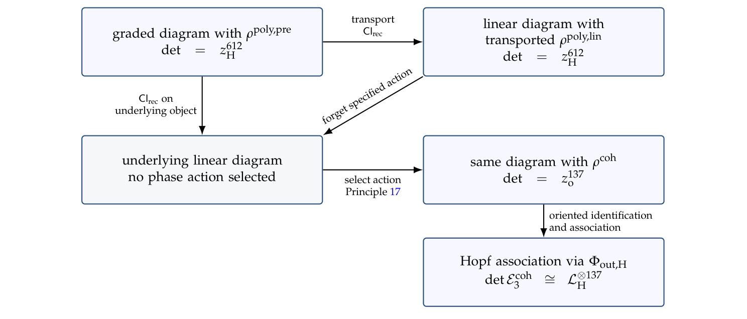
Relations can remove the obstruction of Theorem 16 at the output representation level. Retaining the polynomial phase imposes a stronger restriction.

Theorem 20 (Sharp rotational quotient bounds). Fix a flag \(F\) and its stabilizer \(K\cong(\mathbb{Z}/2\mathbb{Z})^2\). Among \(K\)-equivariant quotients of \(\mathfrak R_3(F)\) whose induced action extends to \(SO(W)\), the largest complex dimension is \(133\). With the coherent scalar circle retained, the same maximum holds for extensions to \(SO(W)\times U(1)_{\mathrm{out}}\). If instead the quotient is \(K\times U(1)_{\mathrm H}\)-equivariant for the polynomial action and must extend to \(SO(W)\times U(1)_{\mathrm H}\), its largest dimension is \(127\). Both maxima are attained.

Under coherent phase, a rank-\(128\) quotient extends precisely when its \(K\)-multiplicities in \((\mathbf1,\chi_1,\chi_2,\chi_3)\) are \((29,33,33,33)\) or \((26,34,34,34)\). The selected quotient \(E_{128}\) of Theorem 17, with multiplicities \((30,34,32,32)\), remains obstructed.

Proof. A \(K\)-module of type \((a,b_1,b_2,b_3)\) extends to \(SO(W)\) if and only if \(b_1=b_2=b_3\). Necessity follows by equating its traces on the three half-turns, which are conjugate in \(SO(W)\). For sufficiency, the complex standard vector representation \(\mathbf3\) restricts to \(\chi_1\oplus\chi_2\oplus\chi_3\), so \(\mathbf1^{\oplus a}\oplus\mathbf3^{\oplus b}\) realizes \((a,b,b,b)\). Semisimplicity of \(K\) implies that quotient multiplicities can be any componentwise smaller nonnegative integers. The maximal extendable quotient therefore has dimension \(a+3\min\{b_1,b_2,b_3\}\). Applying this to \((31,38,34,34)\) gives \(133\); coherent scalar phase adds no restriction.

For polynomial phase, Proposition 23 and Theorem 16 give the following joint multiplicities and rowwise maxima:

Here weight \(3\) combines \(\mathcal Q\otimes\Lambda^1\mathcal I_2\) with \(\Lambda^3\mathcal I_3\); weight \(4\) is \(\mathcal Q\otimes\Lambda^2\mathcal I_2\). The other rows are \(\mathcal Q^{\otimes2}\otimes\overline{\mathfrak B}_1\) and the remaining exterior grades of \(\overline{\mathfrak B}_3\). An invariant kernel splits into circle-weight spaces, and rotations commuting with that circle must preserve each quotient weight space. The criterion therefore applies separately to every row, giving \(96+17+8+3+3=127\). Delete four \(\chi_1\) copies at weight \(5\), two \(\chi_1\) and two \(\chi_2\) copies at weight \(3\), and two \(\chi_3\) copies at weight \(4\) to attain the bound; extend each balanced row by scalar and vector representations with its stated circle weight.

For coherent rank \(128\), the constraints \(a+3b=128\), \(a\leq31\) and \(b\leq34\) give exactly the two displayed types. Their kernels have types \((2,5,1,1)\) and \((5,4,0,0)\), so both occur. The selected quotient has unequal nontrivial multiplicities and fails the criterion. \(\square\)

These are sharp output-representation constraints. They select neither a physical rank nor a preferred kernel, and the attaining subspaces need not be canonical. Extending an output representation does not extend the source spaces and propagation arrows of the full reconstruction diagram. In particular, coherent phase permits rank \(128\) but does not require it.

9.3. Hopf-Associated Reconstruction Bundles

Let \(P_{\mathrm H}=S(S)\to\mathbb{CP}^1\) be the right Hopf principal \(U(1)_{\mathrm H}\)-bundle, and fix \(\Phi_{\mathrm{out,H}}\). For a unitary representation \(\rho:U(1)_{\mathrm H}\to U(V)\), use the inverse-action association convention

This convention is stated only for the circle: its representation images commute, so \(g\mapsto\rho(g)^{-1}\) is a representation and successive identifications agree with multiplication in the structure group.

To check transitions, take local unit sections \(s_a\) with \(s_b=s_a g_{ab}\). For a fixed basis \(v_1,\ldots,v_n\) of \(V\), let \(e_{a,j}=[s_a,v_j]\). The associated local frames satisfy

so fiber coordinates satisfy \(v_a=\rho(g_{ab})^{-1}v_b\). For weight \(w\), the frame transition is \(g_{ab}^{-w}\).

For weight one, view \(p\) as a unit vector spanning its tautological fiber and let \(p^*\) be the complex-linear dual functional on that line with \(p^*(p)=1\). Then \((pg)^*=g^{-1}p^*\), and the fiberwise map

is well defined and identifies the associated line with \(\mathcal T^*=\mathcal L_{\mathrm H}\). Equivalently, the tautological frame transitions are \(s_b=s_a g_{ab}\) and its dual transitions are \(s_b^*=g_{ab}^{-1}s_a^*\). Hence weight \(w\) gives \(\mathcal L_{\mathrm H}^{\otimes w}\) and Chern degree \(w\), using the complex orientation of \(\mathbb{CP}^1\). The opposite association convention reverses all these Chern signs but leaves determinant kernels unchanged.

Transport the coherent representation to \(U(1)_{\mathrm H}\) by

and define

The transported polynomial action already has structure circle \(U(1)_{\mathrm H}\); define likewise

Theorem 21 (Hopf–reconstruction bundle theorem). The coherent associated bundles obey the recursion

and satisfy

In particular,

and

For comparison, the polynomially associated bundle has the decomposition

so \(\det\mathcal E^{\mathrm{poly}}_3\cong\mathcal L_{\mathrm H}^{\otimes612}\).

Proof. Under the coherent action, \(\mathcal Q\) is a trivial phase bundle and each \(\overline{\mathfrak B}_d\) has weight one. Inductively,

which is \(\mathcal L_{\mathrm H}\otimes\underline{\mathfrak R_d}\). The determinant of \(L\otimes\underline{\mathbb{C}_{\mathrm{ph}}^n}\) is \(L^{\otimes n}\). The polynomial decomposition is the bundle version of Eq. (54). \(\square\)

9.4. Determinant-Neutral Closure

Principle 18 (Determinant-neutral epoch closure). After the coherent output has been restricted to a specified fiber, local chart, or pullback along a declared closed comparison cycle, a reconstruction epoch is phase-closed when the coherent action is trivial on the determinant fiber:

This is a constitutive closure criterion. It may later be derived from return of a determinant frame or an equivalent comparison-cycle law, but neither derivation is assumed here.

Definition 20 (Primitive determinant-neutral output phase). By Proposition 23,

Let

Theorem 22 (Determinant-neutral coherent closure). Under common-output coherence, determinant-neutral epoch closure, and the oriented identification \(\Phi_{\mathrm{out,H}}\),

Through \(\Phi_{\mathrm{out,H}}\), the corresponding Hopf-circle subgroup is \(\boldsymbol\mu_{137}^{\mathrm H}\).

Proof. By Proposition 23, the coherent determinant character is \(z_{\mathrm o}\mapsto z_{\mathrm o}^{137}\). Its output-circle kernel is \(\boldsymbol\mu_{137}^{\mathrm{out}}\). Transport through \(\Phi_{\mathrm{out,H}}\) gives \(\boldsymbol\mu_{137}^{\mathrm H}\), and the least positive transported argument is \(2\pi/137\). \(\square\)

Remark 18 (The determinant step is dimension-generic). Let \(V\) be any \(n\)-dimensional complex vector space with the common weight-one scalar action \(z\mapsto z\operatorname{Id}_V\). Then

and determinant neutrality selects the least positive normalized phase \(1/n\) after an orientation is fixed. Thus the architecture-specific content of the present result is the prior construction of a coherent output with \(n=137\), together with the explicit selection of common-output coherence and determinant-neutral closure; the final determinant calculation is universal once those data are in place.

Proposition 25 (What the closure subgroups do not imply). The groups \(\boldsymbol\mu_{137}^{\mathrm{out}}\) and \(\boldsymbol\mu_{137}^{\mathrm H}\) are fiberwise kernels of constant circle representations. By themselves they are not connection holonomies, electromagnetic flux conditions, electron gauge groups, or global reductions of \(\mathcal E^{\mathrm{coh}}_3\) to an \(SU(137)\) bundle. Indeed,

so the determinant line is not globally trivial over \(\mathbb{CP}^1\). A holonomy statement additionally requires a connection and a declared closed path; an electromagnetic statement additionally requires a physical bundle, matter representation, and action normalization.

Proof. The first assertions follow from the definition of a representation kernel. Since \(c_1(\mathcal L_{\mathrm H})\) generates \(H^2(\mathbb{CP}^1;\mathbb{Z})\), Eq. (56) is nonzero. A global \(SU(137)\) reduction would trivialize the determinant line. \(\square\)

9.5. Phase-Role Ledger and Electromagnetic Nonidentification

The mathematical output is denoted \(\vartheta_{137}\) throughout. If the SMM/DTT notation \(\alpha_0:=1/137\) is used for an ideal structural normalization, it abbreviates this value; it does not identify it with a bare QFT coupling, a renormalized coupling, or a measured one. Such an identification requires the action and response realization of §12. The Hopf degree, polynomial determinant weight, coherent determinant weight, and physical electromagnetic coupling answer different questions:

The group actions and their respective roles are summarized in Table 3. This comparison distinguishes an algebraic representation kernel from a connection-dependent holonomy and from the normalization of a physical electromagnetic interaction.

Table 3. Phase groups and representations kept distinct in the reconstruction.

Phase object	Carrier or action	Logical status
\(U(1)_{\mathrm{src}}\)	Minimal faithful real phase carrier and the abstract field \(\mathbb{C}_{\mathrm{ph}}\)	Source representation; linked to dynamics by the phase-identification datum.
\(U(1)_{\mathrm{dyn}}\)	Positive-frequency complex structure \(J_{D}\) on \(\mathcal H_{\mathrm{dyn}}\)	Selected by the published polar-factorization theorem.
\(U(1)_{\mathrm H}\)	Right structure-group action on \(P_{\mathrm H}=S(S)\to\mathbb{CP}^1\)	Geometric theorem; defines the Hopf line.
\(\rho^{\mathrm{poly,pre}}\)	Canonical grading action on the pre-closure reconstruction	Functorially induced; transported by \(\mathsf{Cl}_{\mathrm{rec}}\).
\(\rho^{\mathrm{poly,lin}}\)	Linearized image of \(\rho^{\mathrm{poly,pre}}\)	Determinant weight \(612\) and kernel \(\boldsymbol\mu_{612}^{\mathrm H}\).
\(U(1)_{\mathrm{out}}\) with \(\rho^{\mathrm{coh}}\)	Common weight-one phase on \(\mathcal I_d\), \(\overline{\mathfrak B}_d\), and the receivers	Constitutive output rule; unique only among normalized scalar-diagonal actions.
\(\boldsymbol\mu_{137}^{\mathrm{out}}\)	Output-circle kernel of the coherent determinant	Finite structural closure subgroup under determinant neutrality.
\(\boldsymbol\mu_{137}^{\mathrm H}\)	Image of \(\boldsymbol\mu_{137}^{\mathrm{out}}\) through \(\Phi_{\mathrm{out,H}}\)	Hopf-circle copy; not a holonomy or electromagnetic gauge group.
\(U(1)_{\mathrm{EM}}\)	Physical electromagnetic bundle and matter representation	Unresolved physical matching target.

10. Integrated Reconstruction Theorem and Dependency Ledgers

Theorem 23 (Rank-three, Hopf, free-reconstruction, and phase-separation theorem). Assume:

1. (I1) a recurrent source \(BC_4\) or \(BS^1_{\mathrm g}\) represented by its minimal faithful real carrier;

2. (I2) a real orthogonal flow with the positive-frequency complex structure of Theorem 1, together with an oriented phase-identification datum;

3. (I3) a positive-norm incompatible-phase extension of the selected phase field;

4. (I4) a nonzero center-insensitive record family invariant under connected inner automorphisms;

5. (I5) a complete flag in oriented \(W\) with unoriented proper subspaces, the unital carrier-envelope rule, and the free quadratic-pair completion rule;

6. (I6) the oriented alternating innovation law and the free positive-degree exterior receiver;

7. (I7) global depth-homogeneous completion and independent coproduct adjoining, the polynomial grading with \(\mathcal Q\) in degree two and innovations in degree one, and the chosen linearization \(\mathsf{Cl}_{\mathrm{rec}}=\mathsf{Tot}_{\mathrm{rec}}\circ\mathsf F_{\mathrm{alg}}\).

Then the following conclusions hold. The flag-dependent reconstruction objects, with the transport of Proposition 20, are equivariant over the flag groupoid of Definition 8:

For each supplied flag, Theorem 17 also constructs \(S_2\hookrightarrow\mathfrak R_3\twoheadrightarrow E_{128}\) with \(\dim S_2=9\), \(\dim E_{128}=128\), polynomial determinant weight \(590\), and stabilizer character \((30,34,32,32)\).

When the flag is obtained from the word protocol, Theorem 18 identifies these two ranks as the unique ordered pair under the same completion and comparison rules. The framed reconstruction is initial and has only the identity endomorphism. Every generated linear realization satisfies the rank-defect formula of Theorem 15, and the flag-stabilizer action on the free output has the non-extension obstruction of Theorem 16.

If, in addition,

1. (I8) the common-output coherence requirement of Principle 17 is selected and an oriented output–Hopf identification datum \(\Phi_{\mathrm{out,H}}:U(1)_{\mathrm{out}}\to U(1)_{\mathrm H}\) is supplied,

then

On the selected quotient \(E_{128}\) the same coherent action has determinant \(z_{\mathrm o}^{128}\). If associated to the Hopf circle by the same convention, its determinant line is \(\mathcal L_{\mathrm H}^{\otimes128}\). Selecting its determinant kernel as a closure rule would be an additional quotient-level choice; it is not inferred from a physical change of probe scale. If, further,

1. (I9) determinant-neutral epoch closure from Principle 18 is adopted,

then the admissible output-circle closure phases are \(\boldsymbol\mu_{137}^{\mathrm{out}}\), their Hopf-circle image is \(\boldsymbol\mu_{137}^{\mathrm H}\), and their least positive transported element has normalized phase

The optional word protocol and outer transport of Theorem 4 and Proposition 6 realize one compatible dual-time instance; their scheduling and generator are not forced by (I1)–(I9). No conclusion identifies \(E_{128}\), \(\mathcal L_{\mathrm H}\), \(\mathcal E^{\mathrm{coh}}_3\), \(\boldsymbol\mu_{137}^{\mathrm{out}}\), \(\boldsymbol\mu_{137}^{\mathrm H}\), or \(\vartheta_{137}\) with a physical electron matter line, a \(\mathrm{Spin}^c\) determinant line, an electromagnetic bundle, a connection holonomy, or \(\alpha_{\mathrm{OS}}(0)\).

Proof. The carrier results are Proposition 2, Proposition 3, and Theorem 1. Normed quaternionic rigidity and readout completeness follow from Theorem 2 and Theorem 3. The projective and topological conclusions follow from Proposition 7, Theorem 7, Theorem 8, and Theorem 9. The unital quadratic closure and free exterior branches follow from Proposition 13, Theorem 10, Theorem 11, and Theorem 5. Initiality, framed rigidity, flag equivariance, and dimension \(137\) follow from Theorem 12, Proposition 19, Proposition 20, and Theorem 13. The comparison and flag assertions follow from Theorem 15, Theorem 16, and Theorem 17. The polynomial determinant weight follows from Proposition 23. Under (I8), Proposition 24 and Theorem 21 give Eq. (59). Under (I9), Theorem 22 gives Eq. (60). \(\square\)

10.1. A Finite Example with Both Phase Actions

The following example realizes the hypotheses on explicit spaces and makes the compatibility equations directly inspectable. Its records are linear functionals as in the definition of the record subspace; no physical record-formation procedure is supplied by the example.

Recurrent Source, Flow, and Phase Identifications.

Take \(V_\rho=\mathcal H_{\mathbb{R}}=\mathbb{R}^2\) with its Euclidean inner product and

Then \(\rho\) is faithful, \(\ker D=0\), \(|D|=\omega\operatorname{Id}\), and \(J_{\rho}=J_{D}=J\). The domain of \(D\) and \(|D|\) is all of \(\mathbb{R}^2\). For an abstract field \(\mathbb{C}_{\mathrm{ph}}=\mathbb{R}[i_{\mathrm{ph}}]\), define

Choose \(A=\mathbb{H}\), \(N(a)=a\overline a\), \(j_1=i\), and \(j_2=j\). The norm is positive and multiplicative, the algebra is associative, and \(ij=k=-ji\). This specifies the incompatible-phase extension with overlap \(\eta=0\). Regarding \(\mathbb{H}\) as a right \(\mathbb{C}_{\mathrm{ph}}\)-space through \(\iota_{\mathrm{ph}}\) gives the spinor \(S\cong\mathbb{C}_{\mathrm{ph}}^2\); its unit sphere and projective quotient give the stated Hopf bundle \(S^3\to\mathbb{CP}^1\).

Records, Flag, and Free Receivers.

For \(a=a_0+a_1i+a_2j+a_3k\), let \(\ell_b(a)=a_b\) for \(b=1,2,3\) and set

in the dual coordinate basis. Quaternionic conjugations rotate the imaginary part, so \(\mathcal R\) is invariant under connected inner automorphisms and the kernel of \(r_{\mathcal R}\) is exactly \(\mathbb{R}\mathbf1\). Identify the readout with \(W=\operatorname{Im}\mathbb{H}\), oriented by \((i,j,k)\), and take the flag

The proper subspaces carry no separate orientation. The alternating-word protocol for the separately supplied pair \((i,j)\) instead gives \(\mathbb{R}i\subset\operatorname{span}\{i,k\}\subset W\). Both are admissible flags; this worked receiver uses the displayed \((i,j)\) plane, independently of that optional word schedule. Full rotation covariance of this record family does not assert that rotations fix the distinguished pair \((j_1,j_2)\). Flag transport below acts on the already reconstructed \(W\) and the functors built from it.

Write \(u_0=1\otimes\mathbf1\), \(u_1=1\otimes i\), \(u_2=1\otimes j\), and \(u_3=1\otimes k\). These are vectors in a complexification; the scalar \(i_{\mathrm{ph}}\) is distinct from the quaternionic basis element \(i\). Set

Thus \(\mathcal Q\) has basis \(u_a\odot u_b\) for \(0\leq a\leq b\leq3\) and dimension \(10\). Each \(\mathfrak B_d\) has the exterior-monomial basis \(u_{a_1}\wedge\cdots\wedge u_{a_k}\) for \(1\leq a_1<\cdots<a_k\leq d\). Its generator map is \(\iota_d(v)=v\in\Lambda^1\mathcal I_d\). Give \(\mathcal Q\) degree two and each \(\Lambda^k\mathcal I_d\) degree \(k\). The graded receivers are

Both before and after totalization, the propagation and branch-incidence maps are the summand inclusions

For \(d=1\), the first summand is zero and \(j_1\) is the identity after the canonical identification \(\mathfrak R_1=\overline{\mathfrak B}_1\). In particular,

The dimensions are \((0,1,13,137)\). All spaces carry the induced Hermitian forms and orthogonal direct-sum forms specified in the construction.

Polynomial Action and Its Compatibilities.

For \(z_{\mathrm H}\in U(1)_{\mathrm H}\), multiply \(\mathcal I_d\) by \(z_{\mathrm H}\), \(\mathcal Q\) by \(z_{\mathrm H}^2\), and \(\Lambda^k\mathcal I_d\) by \(z_{\mathrm H}^k\). Denote these maps by \(P_I,P_Q,P_B\) and define the receiver maps recursively by

For homogeneous exterior elements \(b,c\) of degrees \(k,l\), \(P_B(bc)=z_{\mathrm H}^{k+l}bc=(P_Bb)(P_Bc)\). Moreover, \(P_B\iota_d(v)=z_{\mathrm H}\iota_d(v)=\iota_d(P_Iv)\), and Eq. (61) gives directly

Hence this is a unitary automorphism of the unframed graded diagram. Totalizing these same maps gives the transported polynomial action, with the same weights. On \(\mathfrak R_3\), the pairs (dimension, weight) are

in the order of the exterior grades in the three displayed summands. Thus \(\det P_3(z_{\mathrm H})=z_{\mathrm H}^{612}\).

The polynomial action can also be checked on the symmetric pairing \(\beta:\mathcal U_3\times\mathcal U_3\to\mathcal Q\), \(\beta(u,v)=u\odot v\): assigning weight one to \(\mathcal U_3\) gives \(\beta(z_{\mathrm H}u,z_{\mathrm H}v)=z_{\mathrm H}^2\beta(u,v)\). This scalar action on the complexified vector space is not asserted to be a unital algebra automorphism of \(\mathbb{H}\).

Coherent Action and the Structures It Preserves.

For the distinct circle \(U(1)_{\mathrm{out}}\), set

on every nonzero innovation, linear branch, and receiver space. The three linear compatibility checks are

This gives a unitary automorphism of the unframed linear diagram and \(\det C_3(z_{\mathrm o})=z_{\mathrm o}^{137}\). The action is also degree preserving if the construction grading is retained on the underlying vector spaces: every homogeneous component is multiplied by the same scalar. For \(d\geq2\), however,

It therefore fails to preserve branch multiplication for \(z_{\mathrm o}\ne1\). If one additionally required weight one on \(\mathcal U_3\) and compatibility with the symmetric pairing \(\beta\), neutrality of \(\mathcal Q\) would also fail for \(z_{\mathrm o}^2\ne1\). The coherent diagram does not contain \(\mathcal U_3\) or \(\beta\) as retained structure maps: \(\mathcal Q\) is a specified propagator space. Its construction by a symmetric universal property does not require every subsequent linear diagram action to preserve that larger pairing diagram.

Framing and the Additional Closure Test.

For \(z\ne1\), neither action is a framed endomorphism, since its innovation source maps are not identities. Acting by \(z\operatorname{Id}\) on receivers alone also fails the framed relation \(f_1j_1=j_1\), because \(j_1\ne0\). This is consistent with the initial framed diagram having only the identity endomorphism. Finally, choose the oriented identification \(\Phi_{\mathrm{out,H}}(e^{\theta i_{\mathrm{ph}}})=e^{\theta i_{\mathrm{ph}}}\) between the two specified circle copies. If determinant neutrality is adopted as the closure test, the coherent admissible phases are then precisely \(\boldsymbol\mu_{137}^{\mathrm{out}}\), with least positive normalized phase \(1/137\). The determinant character, this chosen test, and the circle identification are separate pieces of the example. No connection holonomy, spatial evolution, or electromagnetic coupling is determined by these finite data.

11. Kinematic Completion and Finite Spectral Amplification

Two distinct extensions are considered here: completed-history calibration can supply a local causal cone, while the finite receiver can enter an independently validated operator geometry as an internal factor. Neither extension follows from a dimension count.

11.1. Completed Propagation and the Euclidean–Lorentzian Bridge

The inner protocol supplies independent tests and the positive spatial readout \(W\cong\operatorname{Im}\mathbb{H}\). A limiting propagation speed concerns a different operation: comparison of completed records. The following conditional extension states the additional calibration and causal assumptions in a fixed local readout. It does not identify the finite word-prefix index with a measured duration.

Definition 21 (Calibrated completed histories). A completed history \(h\) has a dimensionless inner budget \(N(h)\geq0\), an outer duration \(T(h)\geq0\), and a displacement \(x(h)\in W\). These quantities are additive under admissible concatenation in the chosen readout. Fix \(\ell_{\mathrm{in}}>0\) and \(\nu>0\), with units of length and inverse outer time, respectively, and require

Let \(\mathcal C\) be the closed convex cone generated by the increments \((T(h),x(h))\) in \(\mathbb{R}\oplus W\). This cone is a continuum reachability idealization: interpreting its sums, rescalings, and limits as physically accessible macroscopic increments is an additional realization condition.

Theorem 24 (Completion bound and Lorentzian cone). Under Definition 21, set \(c_*=\ell_{\mathrm{in}}\nu\). Every completed increment satisfies \(\left\lVert x(h)\right\rVert\leq c_*T(h)\), and

Suppose, additionally, that the bound is isotropically sharp: for every unit \(n\in W\) there are completed histories with \(T(h)>0\) and \(x(h)/T(h)\longrightarrow c_*n\). Then \(\mathcal C=K_{c_*}^{+}\), and its null boundary, with positivity on the future interior, determines the Lorentzian form

up to a positive scalar. Every invertible linear readout change \(L\) with \(L\mathcal C=\mathcal C\) satisfies \(q(Lv)=\lambda^2q(v)\) for some \(\lambda>0\). Thus the cone automorphisms are Lorentz similitudes; fixing volume scale and spatial orientation, equivalently imposing \(\det L=1\), gives \(SO^+(1,3)\) in the coordinates \((c_*t,x)\).

Proof. The bounds give \(\left\lVert x(h)\right\rVert\leq\ell_{\mathrm{in}}N(h) \leq\ell_{\mathrm{in}}\nu T(h)\). The set \(K_{c_*}^{+}\) is a closed convex cone, so it also contains \(\mathcal C\). Sharpness and closure put every \((1,c_*n)\) in \(\mathcal C\). Their convex hull is the full ball \(\{(1,x):\left\lVert x\right\rVert\leq c_*\}\); conical scaling proves equality.

Write \(y_0=c_*t\) and \(q(Ly)=a y_0^2+2y_0b\cdot y+y^{\mathsf T}Dy\), with \(D\) symmetric. An automorphism of the cone maps its boundary onto itself, so this quadratic polynomial vanishes on \((1,n)\) for every unit \(n\). Comparing \(n\) and \(-n\) gives \(b=0\), and then \(n^{\mathsf T}Dn=-a\) gives \(D=-a\operatorname{Id}\). The future interior is preserved, hence \(a>0\); take \(\lambda=\sqrt a\). Conversely, a positive dilation times a future-preserving Lorentz transformation preserves the cone. Since its determinant has absolute value \(\lambda^4\), the normalization \(\det L=1\) removes both dilation and orientation reversal. The same calculation shows that a quadratic form with this null boundary and positive future interior is a positive multiple of \(q\). \(\square\)

Spatial and Spacetime Symmetries.

The Euclidean metric on \(W\) remains the metric of a constant-time slice. Quaternionic conjugation gives the rest-frame rotation cover \(SU(2)\to SO(3)\); these rotations form the stabilizer of the future unit time vector inside \(SO^+(1,3)\). In an oriented orthonormal frame, the Hermitian matrix \(X=c_*tI_2+\sum\limits_{a=1}^{3}x_a\sigma_a\), with \(\sigma_a\) the Pauli matrices, obeys \(\det X=q(t,x)\). The standard action \(X\mapsto AXA^\dagger\), \(A\in SL(2,\mathbb{C})\), realizes the double cover of \(SO^+(1,3)\) [21]; its \(SU(2)\) subgroup fixes \(I_2\) and recovers spatial rotations. Boosts therefore require the larger noncompact group. No Wick rotation or change of the positive quaternion norm is used: the split form records the causal reach of completed increments. Equivalent inertial readouts must preserve this same sharp cone for the construction to express a relativity principle; a finite-speed bound alone does not make matter dynamics Lorentz covariant. A preferred completion foliation can coexist with this Lorentz-shaped effective cone. On a time–space plane a boost is the hyperbolic rotation \(z\mapsto e^{-\chi j_h}z\) of \(z=c_*t+j_hx_{\parallel}\), \(j_h^2=+1\); this split unit is distinct from the circular phase unit \(i_{\mathrm{ph}}^2=-1\).

The Relative Inner/Outer Rate and Light.

If a calibrated, locally unwrapped inner duration \(\tau\) is supplied, write \(N=\tau/\tau_0\) and \(v_{\mathrm{in}}=\ell_{\mathrm{in}}/\tau_0\). This calibrates the budget; it does not add a completed-event coordinate. In a homogeneous saturated calibration \(T=\tau/(\nu\tau_0)\), the smooth interpolation satisfies

Thus a spatial conversion per inner-time unit multiplies the relative temporal rate; a ratio of two times alone is not a speed. Rescaling \(\tau\) and \(\tau_0\) by the same constant changes the two factors inversely and leaves \(c_*\) unchanged. Without saturation, \(c=\sup_{T(h)>0}\left\lVert x(h)\right\rVert/T(h)\) need only satisfy \(c\leq c_*\). Identifying the sharp \(c\) with the vacuum speed of light requires electromagnetic propagation to reach this boundary and all relevant vacuum sectors to share its calibrated cone. Neither that identification nor an absolute length calibration follows from the structural phase \(\vartheta_{137}=1/137\), the rank-\(128\) comparison, or the relative-rate identity. In SI units the value \(c=299\,792\,458\,\mathrm{m\,s^{-1}}\) is fixed by the metre definition [32]; the present model supplies no independent metrological prediction.

11.2. Persistent Completed Records as an Intended Application

A future model could represent particle persistence by classes of histories whose completed records remain identifiable under continuation and comparison. The present functional space \(\mathcal R\subset A^*\) does not construct such classes. A realization would need the history action, completion and testing procedures, comparison maps, and a physical state space carrying the proposed labels. The finite receiver is therefore considered below only as a possible internal factor of an independently supplied spectral triple [33]; its finite multiplicity does not determine spectral dimension.

Proposition 26 (Finite amplification of a spectral triple). Let \((\mathcal A_T,\mathcal H_T,D_T)\) be a unital spectral triple and let \(F\) be a finite-dimensional Hermitian vector space. Let \(\mathcal A_F\) be any finite-dimensional unital \(*\)-algebra faithfully represented on \(F\). On

one has

so every algebra commutator is bounded, and \(D_T^{(F)}\) has compact resolvent. Wherever the zeta trace is finite,

Hence finite amplification multiplies spectral multiplicity but leaves the summability threshold and spectral dimension unchanged.

Proof. The commutator identity is immediate on the algebraic tensor product. The operator \(D_T^{(F)}\) is the orthogonal direct sum of \(\dim_{\mathbb{C}}F\) copies of \(D_T\), so its resolvent is the corresponding finite direct sum of compact resolvents. Functional calculus gives Eq. (66) by repeating every eigenvalue with multiplicity \(\dim_{\mathbb{C}}F\). \(\square\)

Corollary 9 (Bounded finite internal Dirac perturbation). Suppose in addition that \((\mathcal A_T,\mathcal H_T,D_T,\Gamma_T)\) is even, so \([\Gamma_T,a]=0\) for \(a\in\mathcal A_T\), and \(D_F\) is a self-adjoint operator on \(F\). Then

is a bounded self-adjoint perturbation of \(D_T^{(F)}\). It has compact resolvent, and for \(a\in\mathcal A_T\), \(b\in\mathcal A_F\),

is bounded. Its summability exponent agrees with that of \(D_T\).

Proof. Because \(F\) is finite-dimensional, \(D_F\) and all commutators \([D_F,b]\) are bounded. The Kato–Rellich theorem gives self-adjointness, and compact resolvent is stable under bounded perturbations. Standard singular-value inequalities show that a bounded perturbation does not change the abscissa of convergence of the spectral zeta function; see [34]. \(\square\)

Corollary 10 (Reconstruction receiver as a finite internal factor). Taking \(F=\mathsf{Out}_3(\mathfrak R)\) yields a finite amplification of multiplicity \(137\). It does not produce spectral dimension \(137\), nor does it by itself derive spatial dimension three. Under the coherent-output action, the finite fiber carries the distinguished circle representation with determinant kernel

Under the polynomial action the corresponding kernel is \(\boldsymbol\mu_{612}^{\mathrm H}\); the finite-amplification theorem itself selects neither action. The fiber also retains the branch-propagation decomposition inherited from Eq. (38).

Problem 4 (Temporal crossed-product spectral realization). Construct from recurrent inner order and outer record evolution a valid compact, locally compact, semifinite, or Lorentzian spectral geometry \((\mathcal A_T,\mathcal H_T,D_T)\), and prove the axioms appropriate to the selected category: self-adjointness or Krein self-adjointness, bounded commutators, compactness or local compactness, regularity, summability, and a computed spectral dimension. The represented algebra should consist of bounded observables; unbounded temporal generators should enter \(D_T\) or a precisely stated affiliated-multiplier framework. Then derive, rather than choose, a finite algebra \(\mathcal A_F\) and internal operator \(D_F\) from the filtrations and branch gradings of \(\mathfrak R_3\), and prove that the resulting spectral action or inner fluctuations produce the required physical representations and normalization. The finite amplification and local characteristic construction do not supply this global operator-geometric realization.

Figure 7 illustrates the additional transport problem that remains after finite amplification; its inter-record operator is a future datum.

12. Conditional Reconstruction of Matter and Electromagnetic Response

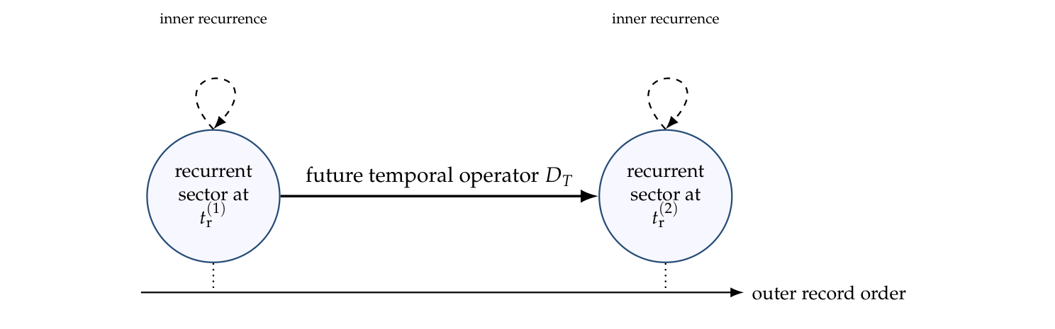
The preceding constructions yield complex phase, a spatial spinor, completion-sector indices, and a calibrated causal cone under their respective hypotheses. This section separates four tasks: realize matter and gauge transport, fix the vacuum response normalization, calculate holonomy and mass dressing, and recover probe-scale dependence within the realized sector. The exact \(137\) and \(128\) label undressed completion templates. A physical coupling is a normalized kinetic response and is not identified with either index or a determinant phase by definition.

12.1. Conservative Boundary Closure

The broader generative–observable interface treats an observed event as an outer closure of an inner recurrent pattern. In a conservative unresolved limit, a physical completion must satisfy

with positivity, normalization, unitarity or complete positivity, relativistic covariance where applicable, and no-signalling retained. The instrument construction in §3.3 gives a finite conservative realization under the trace probability rule; it does not derive that rule or introduce a collapse dynamics.

12.2. A Local Matter–Gauge Realization on the Completed Cone

The completed cone and phase-compatible spinor admit a concrete field-theoretic realization. This is a compatibility construction with specified continuum inputs: it gives equations to be recovered from completion dynamics, rather than leaving the physical interface as a dimension analogy.

Proposition 27 (Compatible matter and electromagnetic characteristics). Supply a smooth contractible four-dimensional patch \(U\) with an oriented, time-oriented coframe \((e^0,e^1,e^2,e^3)\) realizing the calibrated cones of Theorem 24, and set \(g=(e^0)^2-\sum\limits_{a=1}^3(e^a)^2\). Use the selected phase orientation to identify \(\mathbb{C}_{\mathrm{ph}}\) with \(\mathbb{C}\). The spinor \(S\cong\mathbb{C}^2\) of Proposition 7 then supplies the spatial restriction of the two Weyl modules. For a positive orthonormal readout frame \((f_1,f_2,f_3)\), its Pauli operators may be taken as \(\sigma_a=iL_{f_a}\), where \(L_{f_a}\) is left quaternionic multiplication on \(S\). For a cotangent vector with orthonormal components \(p=(p_0,\mathbf p)\), define

These satisfy

Consequently a minimally coupled Dirac operator has precisely the null characteristics of \(g\). A Maxwell kinetic term with constant coefficient \(Z>0\) has the same physical characteristic cone and two transverse polarizations at each nonzero null covector.

Proof. Quaternionic multiplication gives \(\sigma_a\sigma_b=\delta_{ab}I_2+i\epsilon_{abc}\sigma_c\), hence \((\mathbf p\cdot\boldsymbol\sigma)^2=\left\lVert \mathbf p\right\rVert^2 I_2\) gives \(s_+(p)s_-(p)=(p_0^2-\left\lVert \mathbf p\right\rVert^2)I_2\) and all identities in Eq. (69). Polarization yields the Clifford anticommutation relation. Spin and gauge connections, and a mass term, contribute only lower-order terms to the Dirac operator. For Maxwell theory, the principal equation for a potential amplitude \(a\) is \(p^2a^\nu-p^\nu(p\cdot a)=0\), modulo \(a\sim a+\lambda p\), where \(p^2=g^{-1}(p,p)\). If \(p^2\ne0\) every solution is pure gauge; if \(p^2=0\) and \(p\ne0\), the solution quotient is \(p^\perp/\mathbb{C}p\), of complex dimension two. Thus both physical symbols have the claimed cone. Multiplication by \(Z>0\) changes neither conclusion. \(\square\)

In local units \(\hbar=c_*=1\), a corresponding standard effective action is

Here \(\psi\) is a Dirac field, \(\overline\psi=\psi^\dagger\gamma^0\), \(\nabla^{\mathrm{spin}}\) is the Levi–Civita spin connection, and \(q_m\in\mathbb{Z}\) is a supplied circle-representation weight. The connection \(A\) is normalized for a \(2\pi\)-periodic gauge parameter. The transformation \(A\mapsto A-d\chi\), \(\psi\mapsto e^{iq_m\chi}\psi\) leaves the action invariant. This is the usual local Dirac–Maxwell construction [28,35]; its role here is to connect the already constructed phase, spatial spinor, and completed cone in one explicit model. Selecting the continuum patch, the two chiralities, this action, and its quantization remains additional dynamical input. The construction does not supply Einstein evolution, a Born rule, or a vacuum state.

Canonical normalization \(A_{\mathrm{can}}=\sqrt Z\,A\) gives the effective charge \(e_{\mathrm{eff}}=q_m/\sqrt Z\) and, in rationalized natural units,

This is a concrete reconstruction target. The completed-record dynamics must determine the parity-even quadratic gauge response, whose leading local term is the \(F^2\) term in Eq. (70), in a fixed scheme and charge convention. For a unit-weight realization of sector \(\sigma\), a derived \(4\pi Z_\sigma=N_\sigma+\Delta_\sigma\) would yield an inverse coupling. The reference normalization and dressing are separate tasks in §12.5 and §12.6. Choosing that coefficient would only impose the desired value. The structural determinant phase therefore suggests a matching question; the normalized response coefficient is the missing calculation. In this realization electromagnetic fronts propagate on the calibrated cone, so \(c_*\) is its local vacuum light speed; universality across other sectors requires their principal symbols to share that cone.

12.3. Five Physical Matching Targets

Problem 5 (Electron matter-line classification). Construct, independently of empirical coupling input, a physical electron record groupoid \(\mathcal E_e\) and a classifying map

for a Hermitian weight-one matter line \(L_e^{\mathrm{mat}}\). Prove that its class is primitive in the relevant sector. If \(B\mathcal E_e\) is a CW complex of dimension at most two, or if the class has a separately proved primitive-sphere reduction, construct a factorization through \(\mathbb{CP}^1\) and identify

Problem 6 (Connection realization). Construct a physically selected unitary connection \(\nabla_e^{\mathrm{mat}}\) on \(L_e^{\mathrm{mat}}\) and prove that its topological component represents the pullback Chern class, while every exact or dynamical component is derived from electron transport rather than numerical matching.

Problem 7 (\(\mathrm{Spin}^c\) and determinant-line compatibility). If the physical electron sector is \(\mathrm{Spin}^c\), construct its determinant line \(L_e^{\det}\) and prove the exact convention-dependent relation to an external electromagnetic matter line \(L_e^{\mathrm{mat}}\). In the standard convention of Proposition 11, the existence of a weight-one square root is extra structure and must be proved:

No weight-one line follows from the \(\mathrm{Spin}^c\) principal bundle alone.

Problem 8 (Electromagnetic action normalization). Construct the physical electromagnetic principal \(U(1)\) bundle and derive the gauge and matter action in a stated renormalization convention. Prove that the matter representation is normalized so that

Neither the Hopf degree nor either reconstruction determinant action fixes this coefficient.

Problem 9 (Structural-cycle and boundary-response realization). Derive why the physical electron sector selects \(\rho^{\mathrm{coh}}\) rather than \(\rho^{\mathrm{poly,lin}}\), construct the physical output–Hopf identification map, derive determinant-neutral epoch closure from return of a determinant frame or an equivalent comparison-cycle law, and only then identify \(\boldsymbol\mu_{137}^{\mathrm{out}}\subset U(1)_{\mathrm{out}}\) with a concrete closed electron reconstruction cycle. The law by which the structural phase and any finite boundary defect enter the inverse coupling must likewise be derived rather than imposed. The physical response kernel in Proposition 28 must follow from the same dynamics, independently of the coupling value being tested.

Only after Problems 5, 6, 7, 8, and 9 have been solved can the primitive Hopf degree, the coherent structural determinant phase, and a physical electron response be asserted to belong to one electromagnetic object.

12.4. A Conditional Response Mechanism

A response coefficient can be calculated once inner completion supplies a quadratic kernel, rather than inferred from a determinant phase. The next statement is the standard finite-dimensional Gaussian reduction; its role here is to specify a concrete interface from internal records to a gauge response.

Proposition 28 (Eliminating internal completion variables). Let \(V\) and \(H\) be finite-dimensional Hermitian spaces of normalized curvature coefficients \(f\) and internal completion variables \(y\), respectively. Fix \(G=G^*>0\) on \(H\), \(B:V\to H\), and \(\zeta_0>0\), independent of \(f,y\), with \(\zeta_0I-B^*G^{-1}B>0\). For the dimensionless Euclidean action

minimizing over \(y\), or taking \(-\log\int_H\exp(-\mathcal S(f,y))\,dy\) with Lebesgue measure on the underlying real space, gives, up to an \(f\)-independent additive constant in the latter case,

If \(f\) consists of coefficients of \(dA\), this construction is invariant under the Abelian gauge transformation \(A\mapsto A-d\chi\).

Proof. Completing the square replaces the expression in parentheses by \(\langle y+G^{-1}Bf,G(y+G^{-1}Bf)\rangle +\langle f,(\zeta_0I-B^*G^{-1}B)f\rangle\). Translation of the Gaussian variable leaves an \(f\)-independent factor; the minimum occurs at \(y=-G^{-1}Bf\). Gauge invariance follows from \(d(A-d\chi)=dA\). \(\square\)

Suppose the primitive matter charge has been normalized to one, \(D=d+iA\), and the low-momentum kernel has a common local Maxwell form \(\Xi_{\mathrm{eff}}=zI\). Normalize the regulated real curvature modes so that \(\langle f,f\rangle=\int F\wedge *F\) for \(F=dA\) in the Euclidean metric. In rationalized units \(\hbar=c=1\), \(\mathcal S_{\mathrm{Maxwell}}=(8\pi\alpha)^{-1}\int F\wedge *F\); therefore \(\alpha^{-1}=z=4\pi Z\) in the unit-weight normalization of Eq. (71). This provides a calculational route from specified completion dynamics to a coupling. Its physical realization must select \(G,B,\zeta_0\) independently, establish the continuum and regulator limits, and verify locality and unitary Lorentzian continuation. Positivity of a finite matrix alone does not establish these properties or reflection positivity.

Neither \(\zeta_0=137\) nor a response of nine follows from receiver rank. Already for a one-dimensional \(V\), with \(Bf=bf\) and \(G=\lambda I\), the response is \(\lVert b\rVert^2/\lambda\), independently of the dimension of \(H\). The rank-\(9\) comparison sector supplies possible internal channels; its response is nine only under an additional, independently justified normalization of their dynamics and coupling. Likewise, a holonomy phase determines a kinetic coefficient only if a further equation relates them, consistently with Proposition 10. If \(H\) is built from receiver variables, its flag transport must be retained and the resulting response must agree under transported flags; Theorem 16 prevents assuming a fixed-fiber rotation representation. This is the specific construction problem behind the sector-response analysis below.

Geometric phase and kinetic response remain distinct. For example, on the trivial rank-\(m\) Hermitian bundle over \(\mathbb{R}/\mathbb{Z}\), the connection \(d-(2\pi i\theta/m)\operatorname{Id}\,dt\) has determinant holonomy \(e^{2\pi i\theta}\) for arbitrary real \(\theta\). Neither bundle topology nor that phase fixes a Maxwell coefficient. Holonomy constructions [26,36] become coupling calculations only when a selected dynamics relates them to the response kernel.

Corollary 11 (Sign restriction of linear Gaussian elimination). Under Proposition 28, \(\Xi_{\mathrm{eff}}\leq\zeta_0I\). If the result is isotropic, \(\Xi_{\mathrm{eff}}=zI\), then \(0<z\leq\zeta_0\). Thus setting \(\zeta_0=137\) in this model cannot produce a positive correction to \(137\).

Proof. For every \(f\), \(\langle f,B^*G^{-1}Bf\rangle=\left\lVert G^{-1/2}Bf\right\rVert^2\geq0\). Apply the positivity assumption on the Schur complement. \(\square\)

The statement concerns a real linear source coupling with an \(f\)-independent positive kernel. It does not constrain every spectral or interacting correction. In §12.6 the probe enters the Gaussian kernel itself, so the log determinant has a different response mechanism.

12.5. Vacuum Indices and Electromagnetic Normalization

The dual-time interpretation separates a completed vacuum template from its dynamical response. The exact indices \(N_{3|0}=137\) and \(N_{3|2;0}=128\) belong to Definition 16; mass, transport, and holonomy data describe a realization on or between such completed records. This is a sector distinction, not a proposed renormalization-group trajectory. Calling the reference object a vacuum does not by itself select a quantum ground state or the coefficient of \(F^2\).

Proposition 29 (Structural data do not fix the kinetic coefficient). Fix the reconstruction signature, a completion sector, its phase actions and holonomies, a normalized matter covariant derivative \(D=d+iA\), and a Euclidean effective action with Maxwell coefficient \(Z>0\). If the admissible actions permit

then those structural data do not determine \(\alpha^{-1}\). It varies as \(4\pi(Z+\lambda)\) while the dimensions, quotient maps, circle characters, and prescribed connection holonomies remain unchanged.

Proof. The added term is gauge invariant and changes only the parity-even local quadratic coefficient for the prescribed connection. Canonical field normalization, with the matter convention held fixed, gives Eq. (71). None of the algebraic data depends on \(\lambda\). The permitted positive interval therefore contains distinct couplings with identical structural data. \(\square\)

The statement concerns prescribed configurations, not equality of the probability distributions produced by different actions. A microscopic theory can evade this freedom by uniquely fixing its action and matching prescription. The task is to prove that selection, rather than setting the remaining coefficient to a desired integer.

Hypothesis 2 (Trace realization of a vacuum response). For each completed sector \(E_\sigma\), suppose a fixed microscopic prescription yields a Hermitian response operator \(\mathscr{R}_\sigma(\xi)\) on that sector and a scalar local contribution \(z_{\mathrm{loc},\sigma}(\xi)\) such that the normalized, isotropic Maxwell coefficient is

The data \(\xi\) include dimensionless mass ratios, unitary loop transports, the state and the declared matching prescription. Responses transform by conjugation under flag transport. At an independently specified undressed reference \(\xi_*\), suppose

For comparisons of the two sectors, use the same \(r_*,z_*\) and require that the relative-sector response be the compression of the full response. These are realization assumptions, not consequences of the free receiver or its flag covariance.

Theorem 25 (Conditional vacuum-response normalization and dressing). Under Hypothesis 2,

and \(\Delta_\sigma(\xi_*)=0\). If an independent action-normalization result establishes \(r_*=1\) and \(z_*=0\), the reference coefficients are exactly \(137\) and \(128\). More generally their difference is \(9r_*\). At a common deformed configuration with a common local contribution and compressed relative response,

In particular, rank nine alone does not fix this difference. If \(\left\lVert \mathscr{R}_\sigma(\xi)-r_*\operatorname{Id}\right\rVert\leq\epsilon\) and \(|z_{\mathrm{loc},\sigma}(\xi)-z_*|\leq\epsilon_0\), then \(|\Delta_\sigma(\xi)|\leq N_\sigma\epsilon+\epsilon_0\).

Proof. Taking the trace of the scalar reference operator gives \(r_*N_\sigma\). Subtracting the reference yields Eq. (76). Decompose the trace on \(E=K_F\oplus K_F^\perp\) and use the compression assumption to obtain Eq. (77); off-diagonal blocks do not contribute to a trace. For a Hermitian operator on an \(N_\sigma\)-dimensional space, the absolute trace is bounded by \(N_\sigma\) times its operator norm. This gives the last assertion. \(\square\)

This theorem isolates the required physical normalization rather than concealing it in a dimension count. Equality of elementary responses, even if justified by a symmetry of a future kernel, leaves their common magnitude \(r_*\) undetermined. Neither the known flag covariance nor the coherent scalar phase establishes that symmetry. For unit matter weight and a verified Maxwell realization, \(z_\sigma=\alpha_\sigma^{-1}\); before that matching, it is a normalized response functional. The interpretation permits exact vacuum indices together with noninteger dressed coefficients, but does not yet calculate either physical coefficient.

12.6. An Exact Finite Holonomy–Gap Response Model

A finite model shows explicitly how ordered inner transport, outer completion, holonomy, and a positive gap can enter the same response calculation. It is a benchmark for the proposed mechanism. It supplies no microscopic selection of its transport or gap and no automatic identification of its susceptibility with a local Maxwell term.

Let \(E\) be either completed sector, \(N=\dim E\), and let \(U\) be a unitary transport obtained by composing an ordered inner word around a declared closed cycle. In the relative sector, require the descent condition of Theorem 19. At the completed record, apply a dimensionless Abelian probe twist \(\varphi\) and define

Here \(\mu\) is a dimensionless gap. Interpreting it as a mass requires a specified scale, for example \(\mu=m/M_*\), and a derivation of this kernel from the physical dynamics. A basis change conjugates \(U\) and \(K\), so their determinants are invariant. For the complex Gaussian completion variable \(y\in E\) with action \(y^*Ky\), integration gives

The additive constant is independent of \(\varphi\). A fixed reference gap \(\mu_*>0\) defines the dimensionless diagnostic stiffness

The prefactor specifies a reference calibration; it is displayed explicitly and is not claimed to be an electromagnetic normalization theorem.

Proposition 30 (Spectral response, exact reference rank, and controlled dressing). If the eigenvalues of \(U\) are \(e^{i\theta_a}\), then

In particular \(\mathcal Z_N(\operatorname{Id},\mu_*;\mu_*)=N\) and \(\mathcal Z_N(\operatorname{Id},\mu;\mu_*)=N\mu_*^2/\mu^2\). For \(\mu^2=\mu_*^2(1+\varepsilon)\) near \(\mu_*^2\) and small chosen eigenangles,

For fixed \(\mu_*>0\) the remainder is bounded uniformly in a sufficiently small neighborhood. If \(U\) preserves \(K_F\), the unnormalized log determinant and the calibrated stiffness are additive over \(K_F\oplus K_F^\perp\). Hence the reference stiffness difference between the two completion sectors is exactly nine.

Proof. The kernel is positive with eigenvalues \(\mu^2+2-2\cos(\varphi+\theta_a)\geq\mu^2\). The complex Gaussian integral is \(\pi^N/\det K\) in orthonormal coordinates. Twice differentiating its logarithm gives \(2\cos\theta_a/\lambda_a-4\sin^2\theta_a/\lambda_a^2\), proving Eq. (80). At zero eigenangle each summand equals \(\mu_*^2/\mu^2\). Taylor expansion around \((\varepsilon,\theta_a)=(0,0)\) yields Eq. (81); analyticity and the positive gap bound the remainder. Invariance under \(U\) makes \(K\) block diagonal on the two summands, so determinant multiplicativity gives additivity of the logarithm and its derivatives. \(\square\)

This supplies an exact, finite example of integer reference stiffness with continuous holonomy and gap corrections. Small corrections require a controlled neighborhood; they do not follow merely from the words “holonomy” or “mass.” The displayed model gives a negative small-holonomy correction at fixed gap, while a decrease of the gap relative to its reference gives a positive leading correction. These signs are consequences to test, not quantities to adjust to a measured fractional remainder. Positivity of \(K\) does not ensure positivity of the stiffness at every holonomy; a physical stable-response realization must select a domain with positive total coefficient. Only the spectrum of \(U\) enters this particular model. Distinct inner histories with the same completed \(U\) have the same response, so it does not establish observability of the full inner history.

Corollary 12 (One completion product does not fix its dressed response). Holding \(E\), its completion projection, its scalar phase action, and \(U=\operatorname{Id}\) fixed while varying \(\mu>0\) leaves all structural indices and holonomies unchanged but varies \(\mathcal Z_N\) over \((0,\infty)\).

Proof. Use \(\mathcal Z_N=N\mu_*^2/\mu^2\) for \(N>0\). \(\square\)

Thus the example demonstrates the mechanism and its remaining freedom simultaneously. A coupling prediction requires independently selected \(\mu\), \(U\), and a local, normalized electromagnetic action. The next subsection computes the conversion from this susceptibility to a quadratic Maxwell coefficient for one supplied plaquette realization; it does not select that realization. A Wilson-loop susceptibility or a phase potential alone is not the local coefficient. The exact reference rank in Proposition 30 remains a calibrated model result, and Proposition 29 explains why physical normalization is indispensable.

12.7. Response Bounds, Stationarity, and a Specified Local Matching

The positive kernel in Eq. (78) does not by itself make the zero-twist background stationary or its curvature positive. The same finite model nevertheless gives exact restrictions on these questions.

Proposition 31 (Sharp response bound and stationary backgrounds). Let \(N=\dim E\geq1\), \(\mu,\mu_*>0\), and let \(e^{i\theta_j}\) be the eigenvalues of the supplied unitary \(U\). With \(a=\mu^2+2\) and \(c_j=\cos\theta_j\),

with equality exactly when \(U=\operatorname{Id}\). In particular, at \(\mu=\mu_*\) holonomy cannot raise the response above \(N\). If \(\mathcal Z_N=N+\Delta\) with \(\Delta>0\), necessarily \(\mu^2\leq N\mu_*^2/(N+\Delta)\). The zero-twist background is stationary exactly when

An eigenvalue multiset invariant under complex conjugation ensures stationarity. The bound \(\left\lVert U-\operatorname{Id}\right\rVert_{\mathrm{op}}^2<2\mu^2/(\mu^2+2)\) ensures \(\Gamma”_{\mu,U}(0)>0\); together these conditions make zero twist a strict local minimum of the one-variable effective action. For scalar \(U=e^{i\theta}\operatorname{Id}\), stationarity requires \(\theta=0\) or \(\pi\) modulo \(2\pi\), with positive and negative curvature, respectively. Thus the primitive scalar transports \(e^{2\pi i/137}\operatorname{Id}_{137}\) and \(e^{2\pi i/128}\operatorname{Id}_{128}\) are determinant-neutral but not stationary at zero twist in this model.

Proof. Combine the two fractions in Eq. (80). For \(-1\leq c\leq1\),

The bracket is at least \((a-2)(a+4)>0\), so equality requires \(c=1\). Summing proves the bound and its equality case; rearrangement gives the gap restriction. Differentiating \(\Gamma_{\mu,U}(\varphi)=\sum\limits_j\log(a-2\cos(\varphi+\theta_j))\) gives Eq. (83). Conjugate pairs cancel. The norm condition implies \(c_j>2/a\) for every \(j\), making every curvature contribution strictly positive. In the scalar case the derivative is \(2N\sin\theta/(a-2\cos\theta)\); the curvatures at \(0\) and \(\pi\) are \(2N/\mu^2\) and \(-2N/(\mu^2+4)\). \(\square\)

This restriction concerns a proposed identification of a structural scalar phase with the transport entering the kernel; that identification is not assumed. Non-scalar transports such as \(\operatorname{diag}(e^{i\theta},e^{-i\theta},1,\ldots,1)\) provide stationary determinant-one examples, with positive curvature for small \(\theta\) and a strictly smaller response than at \(\theta=0\).

A local quadratic coefficient requires a further specification of how the probe twist represents spacetime curvature. The following example makes that choice and its normalization explicit, using the usual link-holonomy convention [36].

Proposition 32 (Conditional plaquette-to-Maxwell matching). On a flat Euclidean four-torus of side \(\ell\), use cubic spacing \(b=\ell/M\), \(M\in\mathbb{N}\), and \(U(1)\) link variables. For each elementary plaquette \(p=(x;r,s)\), \(r<s\), let \(u_p\) be its oriented link product and supply one variable \(y_p\in E\). Fix the same \(U,\mu\) for all six orientation classes and prescribe the action, with no bare gauge term,

It is gauge invariant, and independent complex Gaussian integration gives \(\Gamma_b[u]=\sum\limits_p\log\det K_p[u]+\mathrm{constant}\). Assume \(\Gamma’_{\mu,U}(0)=0\) and \(\Gamma”_{\mu,U}(0)>0\). For a fixed smooth periodic real one-form \(A\), choose each link as \(\exp(i\int_{\mathrm{link}}A)\) and put \(F=dA\). Then

With unit matter weight, \(D=d+iA\), in rationalized units the inverse coupling associated with this supplied quadratic action is

Proof. Each kernel is at least \(\mu^2\operatorname{Id}\), and its Gaussian integral is \(\pi^N/\det K_p\). The plaquette product is unchanged by site gauge transformations, proving the first assertions. Stokes’ theorem gives \(u_p=e^{i\Phi_p}\) with \(\Phi_p=b^2F_{rs}(x_p)+O(b^4)\) at the plaquette centre, uniformly. Stationarity and Taylor expansion give \(\Gamma_{\mu,U}(\Phi_p)-\Gamma_{\mu,U}(0) =\tfrac12\Gamma”_{\mu,U}(0)\Phi_p^2+O(|\Phi_p|^3)\). There are \(6(\ell/b)^4\) plaquettes, so the summed remainder is \(O(b^2)\). The squared-flux sum tends to \(\int\sum\limits_{r<s}F_{rs}^2=\tfrac12\int\sum\limits_{r,s}F_{rs}^2\). This proves Eq. (84); canonical field normalization in the stated matter convention gives Eq. (85). \(\square\)

At \(U=\operatorname{Id}\) this action gives \(Z_{\mathrm{quad}}=2N/\mu^2\). At \(\mu=\mu_*\), obtaining \(\alpha_{\mathrm{quad}}^{-1}=N\) would therefore require the additional choice \(\mu_*^2=8\pi\). The diagnostic calibration cancels from the physical quadratic coefficient and does not select it. An allowed bare term \(Z_{\mathrm{bare}}\sum\limits_p(1-\operatorname{Re}u_p)\) would add \(Z_{\mathrm{bare}}\) to \(Z_{\mathrm{quad}}\). The proved limit concerns fixed smooth backgrounds in the trivial bundle, with fixed auxiliary data. It does not construct the fluctuating gauge measure, prove reflection positivity or Lorentzian continuation, or determine a renormalized measured coupling. It supplies a conditional local matching while preserving the normalization freedom identified in Proposition 29.

12.8. Sector Selection, Temporal Dressing, and Probe-Scale Evolution

There are three different labels: the completion sector \(\sigma\), the outer completion event \(n\) (or a calibrated outer time), and a probe scale \(Q\) in a renormalization convention \(\mathcal S\). A vacuum-sector index does not run with \(Q\) and does not increase with \(n\). On a physical realization for which Hypothesis 2 and the independent unit normalization hold, the matching target is

The notation allows a time-dependent realization; it does not assert a time-varying measured constant. In a stationary vacuum the relevant data can be independent of \(n\). The undressed reference and its vanishing correction are fixed before physical matching; neither must coincide with the massless limit, \(Q=0\), nor any electroweak scale. The two integers therefore label completed structural vacua, with \(128\) retaining its relative-sector meaning from Definition 16.

If a fixed realized sector recovers ordinary QED, its probe-scale dependence must satisfy the usual renormalization law [28,37]. With all background and state data fixed and within an interval of fixed effective particle content,

Threshold and scheme-conversion terms are additional matching data. This derivative follows from Eq. (86); it is not a derivation of a beta function from rank. Integrating out charged fluctuations also need not implement the algebraic quotient \(E\to E/K_F\). A change of sector requires its own completion-selection mechanism.

The CODATA 2022 recommended low-energy value is \(\alpha_{\mathrm{OS}}^{-1}(0)=137.035\,999\,177(21)\) [38]. Identifying the measured vacuum with \(\sigma=3|0\) would therefore require an independently calculated correction near \(0.035999177\), not a correction defined by subtracting \(137\) from the measurement. The numerical proximity of \(128\) to some electroweak inverse couplings is likewise not evidence for sector selection: the PDG value \([\widehat\alpha^{(5)}(M_Z^2)]^{-1}=127.930\pm0.008\) refers specifically to the five-flavour \(\overline{\mathrm{MS}}\) convention [39, §10.3.1]. No equality between that running coupling and the relative vacuum sector is proposed here.

Problem 10 (A predictive dual-time vacuum realization). Construct one microscopic inner-generation law and outer-completion procedure that: (i) selects the receiver signature and the physically accessible sector; (ii) passes Eq. (49), or supplies the missing outer memory; (iii) selects mass ratios and completion-compatible holonomies; and (iv) fixes the absolute local gauge response and its regulator-independent matching. Derive the correction in Eq. (86), with an error estimate, before comparison with coupling data. If masses are supplied experimentally, state the resulting conditional prediction and check that those inputs do not already determine the coupling being tested. An exact integer plus a freely fitted correction does not solve this problem.

12.9. Empirical Validation

A credible experimental validation program must fix one matching construction before testing it against independent atom-recoil, electron-anomaly, scattering, polarization, and bound-state data, without fitting a separate construction to each observable. The CODATA adjustment provides a reference framework for evaluating fundamental constants [38], while the cesium- and rubidium-recoil studies provide specific precision determinations of the fine-structure constant [40,41]. Schwinger’s paper supplies the historical theoretical calculation of the leading electron magnetic-moment correction [42]; it is not itself a modern precision-measurement report. Failure of any bundle map, line convention, connection, action normalization, unique boundary response, regulator limit, or independence from fitted coupling input falsifies the corresponding physical claim while leaving Theorem 23 intact.

13. Discussion, Comparison, and Limitations

13.1. Which Consequences Depend on the Combined Construction?

The integrated theorem in §10 and the claim-status ledger in Table 1 collect the logical dependencies of the construction. The calculations with arbitrary receivers and flag stabilizers explain why the combined structure contains more information than its dimension.

First, the unique evaluation of the free diagram into any generated receiver converts the absence of relations into an exact equality criterion. By Theorem 15, a relation first imposed at depths one, two, or three has terminal dimension cost weighted by \(100\), \(10\), or \(1\), respectively. The construction in Remark 14 has rank \(127\) and retains the coherent circle while failing to retain the polynomial circle. This directly compares a free object, its linear quotients, and their symmetry constraints.

Second, Theorem 16 separates rotation transport over flags from a rotation representation on one fixed output. The three stabilizer half-turns have traces \(1,-7,-7\), although they are conjugate in \(SO(3)\). Hence a model that requires a flag-independent rotational output with this transport cannot use the free receiver unchanged. It must retain the flag, modify the representation, or change the reconstruction rule. The sharp quotient bounds in Theorem 20 quantify the required modification: at least four dimensions must be removed for an output rotation extension, or ten if rotations commute with inherited polynomial phase. Neither bound singles out \(128\). The obstruction does not prohibit the equivariant bundle over flag space.

Third, Proposition 1 characterizes when a completed readout supports autonomous outer evolution. The word protocol generates a rank-three test family, and conjugation supplies a compatible outer flow. By contrast, right phase multiplication in Proposition 5 can require retaining the scalar coordinate for prediction. This gives both a positive realization and an obstruction for the two temporal roles, without assigning physical duration to word depth. The commutator and stability corollary makes order-sensitive generation quantitative; the completion-cone theorem states exactly which added calibrations yield Lorentzian kinematics.

Fourth, Theorem 17 realizes \(137-9=128\) through an explicit exact sequence. The quotient retains a rotational obstruction, and the alternative natural embedding changes its polynomial determinant weight from \(590\) to \(572\). Neither dimension nor coherent phase alone selects the comparison map. The terminal-defect corollary rules out an earlier-stage deletion under the original propagation signature. Theorem 19 adds a dynamical criterion: the chosen null records must be invariant under the completed transport. Its leakage norm quantifies failure of that condition, while Remark 17 shows why the condition need not hold at intermediate inner steps.

13.2. Focused Comparison with Universal Constructions and Polynomial Methods

The initiality argument uses only the standard universal property of a coproduct and its iteration, as developed in [29,43]. In particular, Theorem 12 is a finite application of that machinery. The conditional characterization in Theorem 14 fixes a signature first and then determines its free receiver. This is the same logical order used for algebraic and many-sorted theories [44]; it supplies no theorem selecting that signature among alternatives.

The symmetric and exterior receivers use the familiar multilinear universal properties and representation constructions in [27]. The literature on algebraic operads [45] provides a broader setting for operations and relations. We neither construct a new operad here nor identify the whole reconstruction with a known free operad. The finite propagation diagram, its framed fiber, and its specified forgetful functors are the objects actually proved to exist.

Joyal’s species viewpoint and its systematic development by Bergeron, Labelle, and Leroux [31,46] explain how sums, products, and compositional descriptions encode counting laws. Our dimension polynomial is similarly obtained after taking dimensions of finite direct sums and tensor products. Exterior signs and flag-stabilizer representations are additional linear information; the integer polynomial alone does not recover them. Thus the numerical identity is an instance of standard counting machinery, whereas the explicit rank-defect comparison and stabilizer non-extension calculation analyze information that this counting forgets.

The positive-frequency theorem, including its common operator domain and bounded-commutant consequence, is proved in Theorem 1 from spectral calculus; its published references supply attribution and wider context. Quantum instruments, the invariant-algebra criterion, the local Dirac–Maxwell construction, and Schur reduction are likewise standard tools applied here to connect the two temporal roles. The autonomous recorder uses standard history-clock and engineered-transfer constructions [17,18]; informational completeness uses the standard instrument framework [16]. Their application here gives a particular word-dependent risk and completion law, not a new general theory of measurement or Hamiltonian computation. Beck’s distributive laws [30] motivate the open compatibility problem in Problem 3; a physical completion monad remains to be constructed.

The log-determinant response uses the spectral theorem and finite Gaussian integration; its derivative is not a new general integration formula. The contribution is its explicit application to the completion-compatible sector family, including exact reference indices, deformation signs, and the distinction between a calibrated susceptibility and an electromagnetic kinetic coefficient. The resulting contribution is an explicit comparison, completion, and obstruction analysis for this selected finite signature. No priority claim is made for the individual classical ingredients, and the broader literature does not independently establish the physical significance of the selected signature or its numerical specialization.

13.3. Precisely What Linearization and Phase Selection Do

Forgetting branch multiplication permits the coherent action on the graded underlying vector spaces. Construction grading itself is compatible with that action, so totalization is an additional information-discarding choice. Retaining the polynomial representation while applying either forgetful step transports the same linear maps and preserves determinant weight \(612\). It does not turn that representation into the coherent one.

Conversely, preserving multiplication and grading alone does not uniquely select a circle action; the polynomial action additionally uses the prescribed generator and propagator weights. The coherent action is uniquely determined only inside the normalized scalar-diagonal class of Proposition 24. Its determinant character \(z\mapsto z^{137}\), the kernel \(\boldsymbol\mu_{137}^{\mathrm{out}}\), and adoption of that kernel as the admissible closure subgroup are three distinct statements. The last requires Principle 18. Only after supplying \(\Phi_{\mathrm{out,H}}\) is the subgroup transported to the Hopf circle and assigned the stated positive phase convention.

13.4. Interpretation and Selection Limits

The reconstruction now has explicit interfaces to quantum records, local spacetime kinematics, and gauge response. Functional tests generate the rank-three readout; the instrument template makes completion probabilistic under the trace rule; the invariant-algebra criterion tests outer autonomy. The calibrated cone and supplied smooth coframe support compatible matter and electromagnetic characteristics. Gaussian elimination calculates a response from a supplied kernel. The holonomy–gap model gives a second, exact spectral response on the same completion sectors. Its reference calibration remains explicit, and Corollary 12 shows why a fixed integer alone cannot select the dressed value. Physical reconstruction requires these ingredients to arise from one selected dynamics, including stable preparations, continuum limits, and a shared cone. The conditional models establish compatibility and expose the remaining selection problems.

The selected unital envelope, free symmetric and alternating receivers, complete-flag depth, full homogeneous propagator, coherent action, and determinant-neutrality criterion remain constitutive. Their operational motivations explain the question being studied, but do not establish that a physical electron or a unique reconstruction theory must realize them. The appendix compares a specified illustrative family of alternatives, not every admissible functor. Because the integers and their numerical proximity to familiar couplings were known during development, neither appearance is a historically independent numerical prediction or independent validation of the selected construction. Their role here is as exact indices of undressed completion templates. The relative rank \(128\) has no assigned electroweak scale, and its proposed dimensional interpretation must respect its explicit depth-two quotient construction. Agreement with a familiar integer cannot replace a selection theorem.

13.5. Next Mathematical and Physical Questions

Further mathematical tasks are to classify relation subspaces preserving both phase actions, select comparison embeddings by an independent principle, select canonical rotational quotients compatible with the full reconstruction arrows, and extend the finite linear and quantum descent criteria to infinite-dimensional systems and records with persistent memory. These questions can be investigated without an electromagnetic interpretation.

The next physical task is to supply a single microscopic completion model that passes three tests: its record channel obeys the declared autonomy or memory law; its continuum matter and gauge symbols share the calibrated cone; and its independently normalized response kernel yields a definite sector-dependent coupling, holonomy/mass dressing, and compatible probe-scale dependence. The receiver signature, charge representation, and regulator must be selected before comparison. §Appendix B records the data to be fixed and the tests that would reject such a realization.

14. Conclusion

The dual-time construction separates ordered inner acquisition from completed outer records. Under the displayed phase, norm, and covariance assumptions, quaternionic words generate a readout flag with dimensions \(1,2,3\) and a quantitative stability bound. A six-outcome instrument realizes these tests on qubits. Its autonomous recorder supplies an exact completion probability and capture window, with finite bandwidth and recurrence. The all-attempt risk separates phase-overlap conditioning from incomplete execution; orthogonal phases minimize it within the specified design. Quantum probabilities, preparations, and apparatus couplings remain supplied operational data.

The central dimensional conclusion is conditional uniqueness of the ordered rank pair \((137,128)\). The completed rank-three carrier, its unital symmetric square, the exterior branches, and homogeneous free propagation give

The specified depth-two comparison has rank \(6\cdot1+3=9\), so its injected image gives the relative rank \(137-9=128\). These counts are independent of basis, admissible phase overlap, and numeral notation. They depend on the declared free-completion and comparison rules. The relative receiver is not a bare two-dimensional receiver, and the rank pair does not itself select a physical vacuum or electromagnetic coupling.

Arbitrary generated receivers satisfy \(\dim X^{\mathrm{gen}}_3=137-100\kappa_1-10\kappa_2-\kappa_3\). Exact outer autonomy and holonomy descent require invariance of the discarded subspace; the finite-horizon bounds quantify residual leakage. The flag obstruction also has a sharp quantitative form: maximal rotational output quotients have ranks \(133\) with coherent phase and \(127\) with commuting polynomial phase. The selected rank-\(128\) relative completion remains obstructed. These output extensions do not establish compatibility of the full reconstruction diagram with flag removal.

Polynomial and coherent phase actions remain distinct, with full-receiver determinant weights \(612\) and \(137\). Determinant neutrality is an additional closure rule and does not normalize a gauge action. The Gaussian model yields exact calibrated stiffness and continuous dressing, but holonomy at fixed reference gap can only lower that stiffness. Stationarity adds a separate constraint on transport. A specified plaquette construction computes the smooth-background Maxwell coefficient and exposes the extra normalization needed to identify an inverse coupling with rank; it does not fix a renormalized measured constant.

The resulting mathematical model connects inner dimensional acquisition, quantum record completion, receiver structure, symmetry, and response through explicit conditional results. The remaining physical task is a microscopic law selecting the completion rules, comparison sector, stable preparations, mass ratios, holonomies, and absolute gauge response. That task remains distinct from the exact structural counts proved here.

Use of Generative AI. During manuscript preparation, the author used OpenAI ChatGPT (OpenAI) to assist with structural reorganization, language editing, mathematical stress-testing, drafting of additional proofs and examples, reference checking, and formatting of an author-developed draft. The author is responsible for independently reviewing and approving all AI-assisted suggestions, mathematical statements, proofs, references, and final wording before submission, and assumes full responsibility for the submitted version.

Conflicts of Interest: The author declares no competing interests.

Data Availability: No datasets were generated or analyzed.

Funding Information: No funding was received for this work.

Appendix A. Alternative Completion and Phase-Action Audit

The comparison class consists of finite complex linear receivers on a height-three flag, built from specified finite branch functors \(B_d\) and propagation spaces \(P_d\) by

Tables 4, 5, and 6 vary, respectively, the branch functor, a constant propagator, and its depth dependence. Tables 7 and 8 compare the phase actions and closure tests on the selected diagram. When multiplication is specified, tensor, symmetric, and exterior truncations use their natural quotient-algebra products. Spinor-based propagators use the separately supplied spinor \(S\); those rows compare dimensions and retain different representation data. The tables are illustrative, not an exhaustive classification of natural functors, quotient relations, heights, or actions. No extremal or unique-selection claim follows from this finite sample.

Table 4 holds the homogeneous propagator \(\mathcal Q\) fixed. Its final row uses an explicitly defined exterior truncation. For every \(d\), the positive exterior algebra modulo its ideal of degrees at least three is

This is an alternating degree-two truncation, not signless bookkeeping; its dimensions are \((0,1,3,6)\).

Table 4. Natural branch completions and the resulting height-three dimensions.

Branch rule	Branch dimensions \((b_0,b_1,b_2,b_3)\)	\(100b_1+10b_2+b_3\)	Status
Linear innovations only	\((0,1,2,3)\)	\(123\)	Omits composite supports.
Free positive exterior completion	\((0,1,3,7)\)	\(137\)	Initial for oriented alternating branch laws.
Truncated symmetric completion \(\bigoplus_{k=1}^{d}\operatorname{Sym}^k I_d\)	\((0,1,5,19)\)	\(169\)	Allows repeated innovations without alternation.
Truncated tensor completion \(\bigoplus_{k=1}^{d}I_d^{\otimes k}\)	\((0,1,6,39)\)	\(199\)	Retains ordered words and repetitions.
Degree-two exterior quotient \(B_d^{\leq2}\)	\((0,1,3,6)\)	\(136\)	Imposes the additional relation that every triple product vanishes.

The table is not evidence for choosing the exterior row. That row is justified only when branch composition is multilinear and oriented-alternating, repeated identical innovations vanish, and no further quotient relations are imposed.

The quadratic closure also has alternatives. Table 5 holds the exterior ladder fixed and changes the propagation object.

Table 5. Alternative propagation objects for the four-dimensional unital complex carrier \(\mathcal U_3\).

Carrier	Complex dimension \(m\)	\(m^2+3m+7\)	Structural interpretation
\(\operatorname{Sym}^2(S)\) for \(\dim_{\mathbb{C}_{\mathrm{ph}}}S=2\)	\(3\)	\(25\)	Symmetric spinor pairs, not all unital carrier pairs.
Linear unital carrier \(\mathcal U_3\) or \(\operatorname{End}_{\mathbb{C}_{\mathrm{ph}}}(S)\)	\(4\)	\(35\)	No quadratic completion.
\(\operatorname{Sym}^2(W_{\mathbb{C}_{\mathrm{ph}}})\) or \(\Lambda^2\mathcal U_3\)	\(6\)	\(61\)	Omits the identity channel or selects alternating pairs.
\(\operatorname{Sym}^2\mathcal U_3\)	\(10\)	\(137\)	Free unordered quadratic pairs on the complete unital carrier.
Ordered pairs \(\mathcal U_3^{\otimes2}\)	\(16\)	\(311\)	Retains ordering as additional data.

The dimension \(10\) is selected by Principle 13 and Principle 14, not by the numerical output. In particular, restoring the identity channel is essential: using \(W_{\mathbb{C}_{\mathrm{ph}}}\) alone gives \(\dim\operatorname{Sym}^2(W_{\mathbb{C}_{\mathrm{ph}}})=6\).

Even after \(\mathcal Q\) and \(\mathfrak B_d\) have been fixed, depth propagation can be varied. Let \(r_0=0\) and adjoin the same branch dimensions \((1,3,7)\). Table 6 displays several rules.

Table 6. Depth-dependent propagation alternatives.

Propagation rule at depth \(d\)	Dimension sequence \((r_0,r_1,r_2,r_3)\)	Depth-three dimension
Homogeneous full closure \(\mathcal Q\otimes-\), \(\dim\mathcal Q=10\)	\((0,1,13,137)\)	\(137\)
Stage-sensitive \(\mathcal Q_d\otimes-\), dimensions \((3,6,10)\)	\((0,1,9,97)\)	\(97\)
Previous-stage \(\mathcal Q_{d-1}\otimes-\), dimensions \((1,3,6)\)	\((0,1,6,43)\)	\(43\)
Incremental graded piece \(\mathcal G_d\otimes-\), dimensions \((2,3,4)\)	\((0,1,6,31)\)	\(31\)
No multiplicative propagation; direct branch accumulation	\((0,1,4,11)\)	\(11\)

Thus the formulation in terms of explicit objects avoids an independent scalar admissibility postulate, while leaving the propagation rule as a separate modeling choice. The depth-homogeneous row is selected only by Principle 16.

Finally, the same reconstruction diagram supports inequivalent phase assignments.

The comparison in Table 7 identifies the weights assigned to the propagator and branches and the resulting output determinant. Equal output dimensions therefore need not imply equal phase representations or equal preserved structure.

Table 7. Phase actions on the reconstruction data.

Action	Weight on \(\mathcal Q\)	Weight on branches	Output determinant
Polynomially induced	\(2\)	\(k\) on \(\Lambda^k\mathcal I_d\)	\(z^{612}\)
Coherent output	\(0\)	\(1\) on innovations and each complete nonempty branch space	\(z^{137}\)
Scalar action after forgetting all diagram data	Not represented	Not represented	\(z^{137}\), but not a diagram symmetry

The coherent row is stronger than a bare scalar action on the forgotten output because it extends to an automorphism of the linear unframed diagram. It is weaker than the polynomial action with respect to the internal exterior-algebra multiplication, which it does not preserve. This is the precise structural choice that any physical boundary-closure theory must justify.

Even after a phase action is selected, the closure test is not automatic. The tests in Table 8 range from identity on every vector to identity only on projective rays. Their different admissible phase sets show why the closure criterion must be stated independently of the selected representation.

Table 8. Alternative phase-closure tests on the depth-three output.

Closure test		Comment
Identity on every output vector	\(\{1\}\)	Too strong to produce a nontrivial finite phase.
Identity on projective rays only	all of \(U(1)\)	Too weak: every scalar acts trivially projectively.
Polynomial determinant neutrality	\(\boldsymbol\mu_{612}^{\mathrm H}\)	Uses the polynomial action, which also survives linearization.
Coherent determinant neutrality	\(\boldsymbol\mu_{137}^{\mathrm{out}}\)	Selected by Principle 17 and Principle 18.

The appearance of \(\boldsymbol\mu_{137}^{\mathrm{out}}\) therefore depends both on the coherent-output action and on determinant neutrality as the declared closure invariant.

Appendix B. Source-Freeze and Model-Selection Protocol

Before any physical comparison, a reproducibility certificate should record and fix the following choices and include hashes of the associated source files:

1. (F1) the source category, phase orientation, and phase-identification maps;

2. (F2) the inner word grammar, acquisition and completion rule, outer evolution, and clock calibration;

3. (F3) the full or relative vacuum-sector identification, selected depth-two embedding, completion projection, outer-autonomy test, and any retained memory;

4. (F4) the unital-envelope rule and the admissible quadratic, branch, and propagation functors;

5. (F5) the reason the free symmetric, positive exterior, and depth-homogeneous constructions are selected over the alternatives in §Appendix A;

6. (F6) whether branch-algebra multiplication is retained or forgotten at boundary closure;

7. (F7) the choice between polynomial and coherent phase actions, the oriented output–Hopf identification map, and the determinant-neutral closure criterion;

8. (F8) the height, complete-flag groupoid, quadratic closure, and depth-three reconstruction receiver;

9. (F9) the electron classifying space, matter line, \(\mathrm{Spin}^c\) convention, electromagnetic bundle, and connections;

10. (F10) the comparison cycle, projector, determinant convention, orientation, and argument branch;

11. (F11) the regulator family, convergence criterion, boundary-response law, probe scale, and renormalization convention;

12. (F12) the reference vacuum, absolute unit-response calibration, allowed local gauge terms, mass-ratio inputs, and holonomy-selection law;

13. (F13) whether a response is a completed-cycle susceptibility or a verified local Maxwell coefficient, and the map relating them;

14. (F14) the complete list of natural alternatives considered before numerical comparison.

The validator that checks these fields must be separate from any script that reads a measured value of the fine-structure constant.