
During the last decades, many developments in harmonic analysis and signal theory showed that despite its power as a fundamental tool for signal analysis, the Fourier transform has limitations in localizing the frequency spectrum of non-stationary signals. To get over this problem, Gabor [1] introduced the short time Fourier transform (STFT). The author considered a nonzero function \(g\in L^2(\mathbb{R}^d)\) called a window and defined the short time Fourier transform of a function \(f \in L^2(\mathbb{R}^d)\) on the so-called time-frequency plan. Even though the short time Fourier transform solved the localization problem, a given window couldn’t be well adapted to study every multi-frequency signals though. To solve this issue, Grossman and Morlet [2] introduced the wavelet transform. The classical wavelet transform of a function \(f \in L^2(\mathbb{R}^d)\) is defined on the so-called time-scale plan \(\mathbb{R}^{\ast}_+\times \mathbb{R}^d\). The classical wavelet transform is closely related to signal theory, for more details we refer the reader to [3,4]. In recent years, many extensions and variants of the wavelet transform have been suggested see, for instance, [5,6]. A further important tool in signal theory, and the main object of the present work, is the multidimensional Fourier–Bessel wavelet transform. This transform is regarded as an extension of the classical wavelet transform associated with the Fourier–Bessel transform. In particular, the Fourier–Bessel wavelet transform has many interesting applications in signal analysis, namely in Laser and ultrasound area [7]. In the last years many works have been interested in studying and developing the harmonic analysis related with this transform [6,8].
In this paper, we denote by \(\mathbb{R}^d_+:=[0,\infty)^d\) and we consider the multidimensional Fourier–Bessel operator [9–11] defined for \(x=(x_1,\dots,x_d)\in \mathbb{R}^d_+\) by \[\Delta_{\alpha}:=\sum^d_{k=1}\left[\frac{\partial^2}{\partial x^2_k}+\frac{2\alpha_k+1}{x_k}\frac{\partial}{\partial x_k}\right].\]
This operator has been studied extensively in both pure and applied mathematics and gives rise to a generalization of multi-variable analytic structures like the Fourier–Bessel transform, the Fourier–Bessel convolution and the Fourier–Bessel wavelet transform [12–15]. Since the harmonic analysis associated with the multidimensional Fourier?Bessel operator has undergone significant development, it is natural to ask whether there exists the equivalent of the scalogram and the Calderón–Toeplitz operators in the multidimensional Fourier–Bessel harmonic analysis setting.
Our goal in the present paper is to present and study the multidimensional Fourier–Bessel wavelet transform in the multidimensional Fourier–Bessel harmonic analysis setting. Furthermore, this article aims to develop two applications of the multidimensional Fourier–Bessel wavelet transform as the scalogram analysis and the Calderón–Toeplitz operators by means of the theory of time frequency analysis. Precisely, let \(L^p_{\alpha}(\mathbb{R}^d_+)\), \(p\in [1,\infty]\), be the space of measurable functions \(f\) on \(\mathbb{R}^d_+\), for which \[\begin{aligned} &&\|f\|_{L^p_{\alpha}(\mathbb{R}^d_+)}:=\left[\int_{\mathbb{R}^d_+}|f(x)|^p\mbox{d}{\mu}_{\alpha}(x)\right]^{1/p}<\infty,\quad p\in [1,\infty),\\ && \|f\|_{L^\infty_{\alpha}(\mathbb{R}^d_+)}:=\mbox{ ess} \sup_{x\in \mathbb{R}^d_+} |f(x)| < \infty, \end{aligned}\] where \(x=(x_1,\ldots,x_d)\) and \[\mbox{d}\mu_{\alpha}(x):=\prod^d_{k=1}\frac{x^{2\alpha_k+1}_k}{2^{\alpha_k}\Gamma(\alpha_k+1)}\mbox{d}x_k.\]
We denote by \(\langle \cdot,\cdot\rangle_{L^2_{\alpha}(\mathbb{R}^d_+)}\) the inner product for \(L^2_{\alpha}(\mathbb{R}^d_+)\).
Specifically, we consider the multidimensional Fourier–Bessel transform \[\mathscr{F}_{\alpha}(f)(\lambda):= \int_{\mathbb{R}^d_+}f(x)j_{\alpha}(\lambda,x)\mbox{d}\mu_{\alpha}(x),\quad \lambda \in \mathbb{R}^d_+,\] where \[j_{\alpha}(\lambda,x):=\prod^d_{k=1}j_{\alpha_k}(\lambda_kx_k),\] with \(j_{\alpha_k}\) is the normalized Bessel function of the first kind and order \(\alpha_k\) (see [16]).
The multidimensional Fourier–Bessel transform can be regarded as a generalization of the Fourier–Bessel transform [17,18]. Many results have already been proved for the multidimensional Fourier–Bessel transform \(\mathscr{F}_{\alpha}\) (see [12,15]).
A function \(g \in L^2_{\alpha}(\mathbb{R}^d_+)\) is called a multidimensional Fourier–Bessel wavelet, if it satisfies for almost all \(\lambda\in \mathbb{R}^d_+\backslash\{0\}\), the admissibility condition \[0<\omega_g:=\int_{\mathbb{R}_+}|\mathscr{F}_{\alpha}(g)(a\lambda)|^2\frac{\mbox{d}a}{a}<\infty.\]
Let \(g \in L^2_{\alpha}(\mathbb{R}^d_+)\) be a multidimensional Fourier–Bessel wavelet. We define for \(f\in L^2_{\alpha}(\mathbb{R}^d_+)\), the multidimensional Fourier–Bessel wavelet transform by \[\Phi_g(f)(a,b):=\int_{\mathbb{R}^d_+}f(y)\overline{\tau_bg_a(y)} \mbox{d}\mu_{\alpha}(y),\quad (a,b) \in \mathbb{R}^{\ast}_+\times \mathbb{R}^d_+,\] where \(\tau_b\) is the multidimensional Fourier–Bessel translation operator (see [12,10]); and \(g_a\) is the dilation function given by the relation \[\mathscr{F}_\alpha(g_a)(\lambda)=\mathscr{F}_\alpha(g)(a\lambda), \quad \lambda\in \mathbb{R}^d_+.\]
Another fundamental tool in time-frequency analysis is the multidimensional Fourier–Bessel wavelet transform, which is the focus of this work.
The present paper provides the following new results in the framework of the multidimensional Fourier–Bessel harmonic analysis:
RKHS structure. We establish that the range of the multidimensional Fourier–Bessel wavelet transform \(\Phi_g\) is a reproducing kernel Hilbert space (RKHS), with an explicit, pointwise bounded kernel \(W_g\) (Theorem 5). This extends previous works [13,14,19] by providing a complete geometric description of the transform range.
Time-frequency operators. For a subset \(U \subset \mathbb{R}_+^{\ast} \times \mathbb{R}_+^d\) of finite \(\eta_\alpha\)-measure, we define the time-frequency operator \(\mathscr{L}_{g,U}\) and prove its boundedness (Theorem 8) and trace-class property (Theorem 9), with explicit trace formula. These operators are the Fourier–Bessel analogue of the classical localization operators studied by Daubechies [20] and Wong [21,22].
Calderón–Toeplitz operators. We introduce Calderón–Toeplitz operators \(T_{g,U}\) in the multidimensional Fourier–Bessel wavelet setting, show their relation with \(\mathscr{L}_{g,U}\), and prove that they are trace-class with a diagonalization in terms of the eigenfunctions of \(\mathscr{L}_{g,U}\) (Theorems 5.1, 5.2 and Remark 2). The theory of Calderón–Toeplitz operators was initiated by Daubechies in [20], developed by Wong [21,22]. Nowadays, Calderón–Toeplitz operators have found many applications in time-frequency analysis, differential equation theory, quantum mechanics. Arguing from this point of view, many works have been done on them, we refer in particular to the article of Balazs et al. [23], (see also [24,25,22,26]).
Scalogram analysis. We define the multidimensional Fourier–Bessel wavelet scalogram \(S_g(f)\) and the subspace scalogram \(\mbox{Scal}_g^V\). Using the spectral decomposition of \(\mathscr{L}_{g,U}\), we derive optimal time-frequency concentration results (Theorem 13) and an accumulated scalogram error estimate (Theorem 14). These results are new even in the one-dimensional Bessel case. We note that the scalogram has many applications; for example, in [27], the authors used the Morlet wavelet scalogram to detect a previously unknown coordinated contractility behavior of the atrium during ventricular fibrillation, a phenomenon that is not captured in a normal electrocardiogram. Other applications can also be found in [28], where the authors applied the scalogram to biomedical signals to detect their short-term temporal interactions.
Numerical illustrations. In the case \(d=2\) and \(\alpha=(\frac{1}{2},\frac{1}{2})\), we provide explicit formulas and numerical visualizations of the Fourier–Bessel wavelet, its transform, and the associated scalogram (Section 7). These examples highlight the non-homogeneous geometry induced by the Fourier–Bessel framework, which differs significantly from the classical Euclidean setting.
These contributions generalize and unify several previous results on Hankel and Bessel wavelet transforms [5,13,14,6,8,19,29] and provide a solid foundation for further applications in signal processing on weighted radial domains.
The paper is organized as follows. In §2, we recall some results about the multidimensional Fourier–Bessel harmonic analysis. In §3 we recall some fundamental results on the multidimensional Fourier–Bessel wavelet transform, and by using the harmonic analysis associated with the operator \(\Delta_{\alpha}\), we show that the range of this integral transform is a reproducing kernel Hilbert space. §4 is devoted to the study of the boundedness and the compactness of the time-frequency operators in this case, and we give a trace formula. In §5, we study the Calderón–Toeplitz operators associated with the multidimensional Fourier–Bessel wavelet transform \(\Phi_g\). In §6, we study the wavelet scalogram associated with the multidimensional Fourier–Bessel wavelet transform \(\Phi_g\). In §7, we present numerical illustrations concerning the multidimensional Fourier–Bessel wavelet transform and its associated wavelet scalogram in the case \(d=2\) and \(\alpha=(\frac{1}{2},\frac{1}{2})\). In the last section, we summarize the obtained results and describe the open questions.
In this section we recall some basic results related to the multidimensional Fourier–Bessel harmonic analysis [12–15,30].
Let \(\alpha=(\alpha_1,\dots,\alpha_d)\in (-\frac{1}{2},\infty)^d\), we denote by \(\Delta_{\alpha}\), the multidimensional Fourier–Bessel operator [9–11] defined for \(x=(x_1,\dots,x_d)\in \mathbb{R}^d_+\) by \[\Delta_{\alpha}:=\sum^d_{k=1}\left[\frac{\partial^2}{\partial x^2_k}+\frac{2\alpha_k+1}{x_k}\frac{\partial}{\partial x_k}\right].\]
For any \(\lambda\in \mathbb{R}^d_+\), the system \[\Delta_{\alpha} u(x)=-|\lambda|^2 u(x),\quad u(0)=1,\quad \frac{\partial}{\partial x_k}u(x)\Big|_{x_k=0}=0,\quad k=1,\ldots,d,\] admits a unique solution \(j_{\alpha}(\lambda,x)\), given by \[j_{\alpha}(\lambda,x):=\prod^d_{k=1}j_{\alpha_k}(\lambda_kx_k),\] where \(j_{\alpha_k}\) is the normalized Bessel function of the first kind and order \(\alpha_k\) (see [16]) given by \[j_{\alpha_k}(x_k):=\Gamma(\alpha_k+1)\sum_{n=0}^\infty \frac{(-1)^n}{n!\Gamma(n+\alpha_k+1)}\left(\frac{x_k}{2}\right)^{2n}.\]
For all \(x,\lambda\in \mathbb{R}^d_+\), the kernel \(j_{\alpha}(\lambda,x)\) satisfies \[|j_{\alpha}(\lambda,x))|\leq 1.\]
The kernel \(j_{\alpha}(\lambda,x)\) gives rise to an integral transform, which is called multidimensional Fourier–Bessel transform on \(\mathbb{R}^d_+\), where many basic properties had been established [9]. The multidimensional Fourier–Bessel transform \(\mathscr{F}_{\alpha}\) is defined for \(f\in L^1_{\alpha}(\mathbb{R}^d_+)\) by \[\mathscr{F}_{\alpha}(f)(\lambda):=\int_{\mathbb{R}^d_+}f(x)j_{\alpha}(\lambda,x)\mbox{d}{\mu}_{\alpha}(x),\quad \lambda\in\mathbb{R}^d_+.\]
Moreover if \(f\in L^1_{\alpha}(\mathbb{R}^d_+)\), then \[\|\mathscr{F}_{\alpha}(f)\| _{L^\infty_{\alpha}(\mathbb{R}^d_+)}\leq \|f\|_{L^1_{\alpha}(\mathbb{R}^d_+)}.\]
Theorem 1. [12]
(i) Plancherel formula for \(\mathscr{F}_{\alpha}\). The transform \(\mathscr{F}_{\alpha}\) extends uniquely to an isometric isomorphism on \(L^2_{\alpha}(\mathbb{R}^d_+)\), onto itself. In particular, \[\|\mathscr{F}_{\alpha}(f)\|_{L^2_{\alpha}(\mathbb{R}^d_+)}=\|f\|_{L^2_{\alpha}(\mathbb{R}^d_+)}.\]
(ii) Parseval formula for \(\mathscr{F}_{\alpha}\). For all \(f,g\in L^2_{\alpha}(\mathbb{R}^d_+)\), we have \[\langle \mathscr{F}_{\alpha}(f),\mathscr{F}_{\alpha}(g)\rangle_{L^2_{\alpha}(\mathbb{R}^d_+)}=\langle f,g\rangle_{L^2_{\alpha}(\mathbb{R}^d_+)}.\]
(iii) Inversion formula for \(\mathscr{F}_{\alpha}\). If \(f\) and \(\mathscr{F}_{\alpha}(f)\) are both in \(L^1_{\alpha}(\mathbb{R}^d_+)\), then \[f(x)=\int_{\mathbb{R}^d_+}\mathscr{F}_{\alpha}(f)(\lambda)j_{\alpha}(\lambda,x)\mbox{d}\mu_{\alpha}(\lambda),\quad \mbox{a.e} \quad x\in \mathbb{R}^d_+,\] and \[\mathscr{F}^{-1}_{\alpha}(f)(x)=\mathscr{F}_{\alpha}(f)(x).\]
We denote by \(C_{\ast}(\mathbb{R}^d_+)\), the space of continuous functions \(f\) on \(\mathbb{R}^d_+\), even with respect to each variable. For \(f\in C_{\ast}(\mathbb{R}^d_+)\) and \(x,y\in \mathbb{R}^d_+\), we define the multidimensional Fourier–Bessel translation operator (see [12,10]) by \[\tau_x f(y):=a_{\alpha}\int_{(0,\pi)^d}f\left([x_1,y_1]_{\theta_1},\ldots,[x_d,y_d]_{\theta_d}\right)\times \prod^d_{k=1}(\sin \theta_k)^{2\alpha_k}\mbox{d}\theta_1\ldots \mbox{d}\theta_d,\tag{1}\] where \([x_i,y_i]_{\theta_i}:=\sqrt{x^2_i+y^2_i+2x_iy_i\cos \theta_i}\), \(i=1,\ldots,d\) and \(a_{\alpha}:=\displaystyle\prod^d_{k=1}\frac{\Gamma(\alpha_k+1)}{\sqrt{\pi}\Gamma(\alpha_k+1/2)}\).
For suitable function \(f\), for all \(x,y \in \mathbb{R}^d_+\), we have \[\tau_x f(y)= \tau_y f(x) \quad \mbox{and} \quad \tau_0 f(x)=f(x).\]
For all \(\lambda,x, y \in \mathbb{R}^d_+\), we have the product formula \[\tau_x(j_{\alpha}(\lambda,\cdot))(y)=j_{\alpha}(\lambda,x) j_{\alpha}(\lambda,y).\]
For \(f \in L^p_{\alpha}(\mathbb{R}^d_+)\), \(p\in [1, \infty]\), and \(x \in \mathbb{R}^d_+\), then \(\tau_x f \in L^p_{\alpha}(\mathbb{R}^d_+)\) and \[\left\|\tau_xf\right\|_{L^p_{\alpha}(\mathbb{R}^d_+)} \leq\|f\|_{L^p_{\alpha}(\mathbb{R}^d_+)}.\]
For \(f \in L^p_{\alpha}(\mathbb{R}^d_+)\), \(p=1,2\) and \(x \in \mathbb{R}^d_+\), we have \[\mathscr{F}_{\alpha}\left(\tau_x f\right)(\lambda)=j_{\alpha}(\lambda,x) \mathscr{F}_{\alpha}(f)(\lambda), \quad \lambda \in \mathbb{R}_{+}^d.\]
Let \(f,g\in L^2_{\alpha}(\mathbb{R}^d_+)\). The multidimensional Fourier–Bessel convolution product (see [12]) of \(f\) and \(g\) is defined by \[f\ast g(x):=\int_{\mathbb{R}^d_+}f(y)\tau_xg(y) \mbox{d}\mu_{\alpha}(y),\quad x\in \mathbb{R}^d_+.\tag{2}\]
The convolution \(\ast\) is commutative, associative and satisfies the Young inequality (see [12]). Let \(p,q,r\in[1,\infty]\) such that \(\frac{1}{p}+\frac{1}{q}=1+\frac{1}{r}\). Then for \(f\in L^p_{\alpha}(\mathbb{R}^d_+)\) and \(g\in L^q_{\alpha}(\mathbb{R}^d_+)\) we have \[\|f\ast g\|_{L^{r}_{\alpha}(\mathbb{R}^d_+)}\leq \|f\|_{L^p_{\alpha}(\mathbb{R}^d_+)}\|g\|_{L^q_{\alpha}(\mathbb{R}^d_+)}.\]
Theorem 3. [14]
For \(f,g\in L^2_{\alpha}(\mathbb{R}^d_+)\), the function \(f\ast g\) belongs to \(L^{\infty}_{\alpha}(\mathbb{R}^d_+)\), and \[f\ast g=\mathscr{F}^{-1}_{\alpha}(\mathscr{F}_{\alpha}(f)\mathscr{F}_{\alpha}(g)).\]
Let \(f,g\in L^2_{\alpha}(\mathbb{R}^d_+)\). Then \(f\ast g\) belongs to \(L^2_{\alpha}(\mathbb{R}^d_+)\) if and only if \(\mathscr{F}_{\alpha}(f)\mathscr{F}_{\alpha}(g)\) belongs to \(L^2_{\alpha}(\mathbb{R}^d_+)\), and \[\mathscr{F}_{\alpha}(f \ast g)= \mathscr{F}_{\alpha}(f)\mathscr{F}_{\alpha}(g),\quad \mbox{ in the } L^2_{\alpha}(\mathbb{R}^d_+)-\mbox{case}.\]
Let \(f,g\in L^2_{\alpha}(\mathbb{R}^d_+)\). Then \[\int_{\mathbb{R}^d_+}|f \ast g(x)|^2\mbox{d}\mu_{\alpha}(x) = \int_{\mathbb{R}^d_+}|\mathscr{F}_{\alpha}(f)(\lambda)|^2 |\mathscr{F}_{\alpha}(g)(\lambda)|^2 \mbox{d}\mu_{\alpha}(\lambda),\] where both sides are finite or infinite.
In this section, we first recall some fundamental results on the multidimensional Fourier–Bessel wavelet transform. This transform has been investigated in depth in [13,14,19,29] in which precise definitions, examples, and a more complete discussion of its properties can be found. By using the harmonic analysis associated with the operator \(\Delta_{\alpha}\), we show that the range of this integral transform is a reproducing kernel Hilbert space (RKHS).
Let \(g\in L^2_{\alpha}(\mathbb{R}^d_+)\), and \(a>0\). The function \(g_a\) given by \[g_a(x)=\frac{1}{a^{2(\langle\alpha\rangle+d)}}g\left(\frac{x}{a}\right),\quad x\in \mathbb{R}^d_+,\] satisfies \[\mathscr{F}_{\alpha}(g_a)(\lambda)=\mathscr{F}_{\alpha}(g)(a\lambda), \quad \lambda\in \mathbb{R}^d_+,\] and \[\|g_a\|_{L^2_{\alpha}(\mathbb{R}^d_+)}= \frac{1}{a^{\langle\alpha\rangle+d}}\|g\|_{L^2_{\alpha}(\mathbb{R}^d_+)},\tag{3}\] where \(\langle\alpha\rangle=\alpha_1+\alpha_2+\cdots+\alpha_d\).
We say that a function \(g \in L^2_{\alpha}(\mathbb{R}^d_+)\) is a multidimensional Fourier–Bessel wavelet, if it satisfies for almost all \(\lambda\in \mathbb{R}^d_+\backslash\{0\}\), the admissibility condition \[0<\omega_g:=\int_{\mathbb{R}^{\ast}_+}|\mathscr{F}_{\alpha}(g)(a\lambda)|^2\frac{\mbox{d}a}{a}<\infty.\tag{4}\]
Condition (4) is well known in the literature [13,14,19], and the constant
\(\omega_g\) is independent of \(\lambda\).
Example 1. The function \(g\) given by \[g(x):=\int_{\mathbb{R}^d_+}|\lambda|^2e^{-|\lambda|^2}j_{\alpha}(\lambda,x)\mbox{d}\mu_{\alpha}(\lambda),\quad x\in \mathbb{R}^d_+,\] is a multidimensional Fourier–Bessel wavelet and \(\omega_g=\frac{1}{8}\).
For a function \(g \in L^2_{\alpha}(\mathbb{R}^d_+)\) and for \((a,b) \in \mathbb{R}^{\ast}_+\times \mathbb{R}^d_+\) we denote by \(g_{a,b}\) the function defined on \(\mathbb{R}^d_+\) by \[g_{a,b}(x) :=\tau_bg_a(x),\] where \(\tau_b\) are the multidimensional Fourier–Bessel translation operators given by (1).
From Theorem 2 (iii) and (3) the function \(g_{a,b}\) satisfies \[\|g_{a,b}\|_{L^2_{\alpha}(\mathbb{R}^d_+)}\leq \frac{1}{a^{\langle\alpha\rangle+d}}\|g\|_{L^2_{\alpha}(\mathbb{R}^d_+)}.\tag{5}\]
Let \(g \in L^2_{\alpha}(\mathbb{R}^d_+)\) be a multidimensional Fourier–Bessel wavelet. We define for \(f\in L^2_{\alpha}(\mathbb{R}^d_+)\), the multidimensional Fourier–Bessel wavelet transform by \[\Phi_g(f)(a,b):=\langle f,g_{a,b}\rangle_{L^2_{\alpha}(\mathbb{R}^d_+)}= \int_{\mathbb{R}^d_+}f(x)\overline{g_{a,b}(x)}\mbox{d}\mu_{\alpha}(x),\tag{6}\] which can also be written in the form \[\Phi_g(f)(a,b)=f\ast\overline{g_a}(b),\tag{7}\] where \(\ast\) is the multidimensional Fourier–Bessel convolution product given by (2).
From (5) and (6) with Hölder’s inequality we have \[\|\Phi_g(f)(a,\cdot)\|_{\infty}\leq \frac{1}{a^{\langle\alpha\rangle+d}}\|f\|_{L^2_{\alpha}(\mathbb{R}^d_+)}\|g\|_{L^2_{\alpha}(\mathbb{R}^d_+)}.\tag{8}\]
We denote by \(L^p_{\alpha}(\mathbb{R}^{\ast}_+\times \mathbb{R}^d_+)\), \(p\in [1,\infty)\), the space of measurable functions \(f\) on \(\mathbb{R}^{\ast}_+\times \mathbb{R}^d_+\), such that \[\|f\|_{L^p_{\alpha}(\mathbb{R}^{\ast}_+\times \mathbb{R}^d_+)}:=\left[\int_{\mathbb{R}^{\ast}_+}\int_{\mathbb{R}^d_+}|f(a,b)|^p\mbox{d}\mu_{\alpha}(b)\frac{\mbox{d}a}{a}\right]^{1/p} <\infty.\]
We denote by \(\langle \cdot,\cdot\rangle_{L^2_{\alpha}(\mathbb{R}^{\ast}_+\times \mathbb{R}^d_+)}\) the inner product for \(L^2_{\alpha}(\mathbb{R}^{\ast}_+\times \mathbb{R}^d_+)\).
Theorem 4. Let \(g \in L^2_{\alpha}(\mathbb{R}^d_+)\) be a multidimensional Fourier–Bessel wavelet.
Plancherel formula for \(\Phi_g\). For \(f \in L^2_{\alpha}(\mathbb{R}^d_+)\) we have \[\|f\|^2_{L^2_{\alpha}(\mathbb{R}^d_+)}=\frac{1}{\omega_g}\|\Phi_g(f)\|^2_{L^2_{\alpha}(\mathbb{R}^{\ast}_+\times \mathbb{R}^d_+)}.\]
Parseval formula for \(\Phi_g\). For \(f,h \in L^2_{\alpha}(\mathbb{R}^d_+)\) we have \[\langle f,h\rangle_{L^2_{\alpha}(\mathbb{R}^d_+)}=\frac{1}{\omega_g}\langle \Phi_g(f),\Phi_g(h)\rangle_{L^2_{\alpha}(\mathbb{R}^{\ast}_+\times \mathbb{R}^d_+)}.\]
Proof. (i) Using Fubini–Tonelli’s theorem, Theorem 3 (iii), and the relation (7), we obtain \[\begin{aligned} \frac{1}{\omega_g}\|\Phi_g(f)\|^2_{L^2_{\alpha}(\mathbb{R}^{\ast}_+\times \mathbb{R}^d_+)}&= \frac{1}{\omega_g}\int_{\mathbb{R}^{\ast}_+}\int_{\mathbb{R}^d_+}|f\ast \overline{g_a}(b)|^2\mbox{d}\mu_{\alpha}(b)\frac{\mbox{d}a}{a}\\ &= \frac{1}{\omega_g}\int_{\mathbb{R}^{\ast}_+}\int_{\mathbb{R}^d_+}|\mathscr{F}_{\alpha}(f)(\lambda)|^2|\mathscr{F}_{\alpha}(\overline{g_a})(\lambda)|^2\mbox{d}\mu_{\alpha}(\lambda)\frac{\mbox{d}a}{a} \\&=\int_{\mathbb{R}^d_+}|\mathscr{F}_{\alpha}(f)(\lambda)|^2\left[\frac{1}{\omega_g}\int_{\mathbb{R}^{\ast}_+}|\mathscr{F}_{\alpha}(g)(a\lambda)|^2\frac{\mbox{d}a}{a}\right] \mbox{d}\mu_{\alpha}(\lambda). \end{aligned}\]
By relation (4) we have \[\frac{1}{\omega_g}\int_{\mathbb{R}^{\ast}_+}|\mathscr{F}_{\alpha}(g)(a\lambda)|^2\frac{\mbox{d}a}{a}=1.\] Then we deduce the desired result from Theorem 1 (i).
(ii) The result is easily deduced from (i). ◻
Theorem 5. Let \(g\in L^2_{\alpha}(\mathbb{R}^d_+)\) be a multidimensional Fourier–Bessel wavelet. The space \(\Phi_g(L^2_{\alpha}(\mathbb{R}^d_+))\) is a reproducing kernel Hilbert space with kernel function \[W_g((a,b);(a’,b’))=\frac{1}{\omega_g}\langle g_{a,b},g_{a’,b’}\rangle_{L^2_{\alpha}(\mathbb{R}^d_+)}.\]
Moreover, the kernel \(W_g\) is pointwise bounded and for all \((a,b), (a’,b’) \in \mathbb{R}^{\ast}_+\times \mathbb{R}^d_+\), \[|W_g((a,b);(a’,b’))|\leq \frac{1}{\omega_g(aa’)^{\langle\alpha\rangle+d}}\|g\|^2_{L^2_{\alpha}(\mathbb{R}^d_+)}.\]
Proof. From (6) we have \[W_g((a,b);(a’,b’))=\frac{1}{\omega_g}\Phi_g(g_{a,b})(a’,b’).\tag{9}\]
Then, from (5) for every \((a,b)\in \mathbb{R}^{\ast}_+\times \mathbb{R}^d_+\), the function \(g_{a,b}\) belongs to \(L^2_{\alpha}(\mathbb{R}^d_+)\) and therefore the function \(W_g((a,b);\cdot)\) belongs to \(\Phi_g(L^2_{\alpha}(\mathbb{R}^d_+))\).
Moreover by (9), Theorem 4 (i) we have \[\|W_g((a,b);\cdot)\|^2_{L^2_{\alpha}(\mathbb{R}^{\ast}_+\times \mathbb{R}^d_+)} =\frac{1}{\omega^2_g}\|\Phi_g(g_{a,b})\|^2_{L^2_{\alpha}(\mathbb{R}^{\ast}_+\times \mathbb{R}^d_+)} =\frac{1}{\omega_g}\|g_{a,b}\|^2_{L^2_{\alpha}(\mathbb{R}^d_+)}<\infty.\]
On the other hand, from (6) and Theorem 4 (ii) we have \[\begin{aligned} \Phi_g(f)(a,b)&=\langle f,g_{a,b}\rangle_{L^2_{\alpha}(\mathbb{R}^d_+)}\\ &=\frac{1}{\omega_g}\langle\Phi_g(f),\Phi_g(g_{a,b})\rangle_{L^2_{\alpha}(\mathbb{R}^{\ast}_+\times \mathbb{R}^d_+)} \\&=\langle \Phi_g(f),W_g((a,b);\cdot)\rangle_{L^2_{\alpha}(\mathbb{R}^{\ast}_+\times \mathbb{R}^d_+)}. \end{aligned}\]
We conclude that \(W_g((a,b);(a’,b’))\) is a reproducing kernel of the Hilbert space \(\Phi_g(L^2_{\alpha}(\mathbb{R}^d_+))\).
Finally, from Hölder’s inequality and (5) we obtain \[|W_g((a,b);(a’,b’))|\leq \frac{1}{\omega_g}\|g_{a,b}\|_{L^2_{\alpha}(\mathbb{R}^d_+)}\|g_{a’,b’}\|_{L^2_{\alpha}(\mathbb{R}^d_+)} \leq \frac{1}{\omega_g(aa’)^{\langle\alpha\rangle+d}}\|g\|^2_{L^2_{\alpha}(\mathbb{R}^d_+)}.\]
The theorem is proved. ◻
For \(f\in L^2_{\alpha}(\mathbb{R}^d_+)\) and \(F\in L^2_{\alpha}(\mathbb{R}^{\ast}_+\times \mathbb{R}^d_+)\), we define the operator \(\Phi^{\ast}_g\) by the relation \[\langle\Phi_g(f),F\rangle_{L^2_{\alpha}(\mathbb{R}^{\ast}_+\times \mathbb{R}^d_+)}=\omega_g\langle f,\Phi^{\ast}_g(F)\rangle_{L^2_{\alpha}(\mathbb{R}^d_+)}.\tag{10}\]
Theorem 6. Let \(g \in L^{2}_{\alpha}(\mathbb{R}^d_+)\) be a multidimensional Fourier–Bessel wavelet.
For every \(f\in L^2_{\alpha}(\mathbb{R}^d_+)\), we have \[\Phi^{\ast}_g\Phi_g(f)(x)=f(x), \quad x\in \mathbb{R}^d_+.\]
For every \(F\in \Phi_g(L^2_{\alpha}(\mathbb{R}^d_+))\), we have \[\Phi_g\Phi^{\ast}_g(F)(a,b)=F(a,b), \quad (a,b)\in \mathbb{R}^{\ast}_+\times \mathbb{R}^d_+.\]
Proof. (i) For every \(f\in L^{2}_{\alpha}(\mathbb{R}^d_+)\), we have \[\langle \Phi^{\ast}_g\Phi_g(f),f\rangle_{L^{2}_{\alpha}(\mathbb{R}^d_+)}=\frac{1}{\omega_g}\langle \Phi_g(f),\Phi_g(f)\rangle_{L^2_{\alpha}(\mathbb{R}^{\ast}_+\times \mathbb{R}^d_+)}=\langle f,f\rangle_{L^{2}_{\alpha}(\mathbb{R}^d_+)}.\]
Then \(\Phi^{\ast}_g\Phi_g(f)=f\).
(ii) For every \(F\in \Phi_g(L^2_{\alpha}(\mathbb{R}^d_+))\), there exists \(f\in L^{2}_{\alpha}(\mathbb{R}^d_+)\) such that \(\Phi_g(f)=F\). Then by (i) we obtain \[\Phi_g\Phi^{\ast}_g(F)=\Phi_g\Phi^{\ast}_g\Phi_g(f)=\Phi_g(f)=F.\]
The theorem is proved. ◻
Theorem 7. Let \(g \in L^{2}_{\alpha}(\mathbb{R}^d_+)\) be a multidimensional Fourier–Bessel wavelet. For \(F\in L^2_{\alpha}(\mathbb{R}^{\ast}_+\times \mathbb{R}^d_+)\) we have \[\Phi_g\Phi^{\ast}_g(F)(a,b)=\langle F,W_g((a,b);\cdot)\rangle_{L^2_{\alpha}(\mathbb{R}^{\ast}_+\times \mathbb{R}^d_+)},\quad (a,b)\in \mathbb{R}^{\ast}_+\times \mathbb{R}^d_+.\]
Proof. Let \(F\in L^2_{\alpha}(\mathbb{R}^{\ast}_+\times \mathbb{R}^d_+)\). From (10) and Theorem 6 (ii) we have \[\begin{aligned} \Phi_g\Phi^{\ast}_g(F)(a,b)&=\langle \Phi_g\Phi^{\ast}_g(F),W_g((a,b);\cdot)\rangle_{L^2_{\alpha}(\mathbb{R}^{\ast}_+\times \mathbb{R}^d_+)}\\&= \langle F,\Phi_g\Phi^{\ast}_g(W_g((a,b);\cdot))\rangle_{L^2_{\alpha}(\mathbb{R}^{\ast}_+\times \mathbb{R}^d_+)} \\&=\langle F,W_g((a,b);\cdot)\rangle_{L^2_{\alpha}(\mathbb{R}^{\ast}_+\times \mathbb{R}^d_+)}. \end{aligned}\]
The theorem is proved. ◻
In this section, we define the time-frequency operators for the multidimensional Fourier–Bessel wavelet transform and we prove that they are bounded and compact operators in the so-called Schatten-von Neumann classes, the proofs are inspired from related results in [22]. In the following, \(g\) is a multidimensional Fourier–Bessel wavelet such that \(\|g\|_{L^2_{\alpha}(\mathbb{R}^d_+)}=1\).
We denote by \(B(L^2_{\alpha}(\mathbb{R}^d_+))\) the space of all bounded operators \(\Psi\) from \(L^2_{\alpha}(\mathbb{R}^d_+)\) into itself, equipped with the norm \[\|\Psi\|:=\sup_{\|f\|_{L^2_{\alpha}(\mathbb{R}^d_+)}=1}\|\Psi(f)\|_{L^2_{\alpha}(\mathbb{R}^d_+)}.\]
For a compact operator \(\Psi\in B(L^2_{\alpha}(\mathbb{R}^d_+))\), the eigenvalues of the positive self-adjoint operator \(|\Psi|:=\sqrt{\Psi^*\Psi}\) are called the singular values of \(\Psi\) and denoted by \(\lbrace s_n(\Psi)\rbrace_{n\in \mathbb{N}}\).
The Schatten-von Neumann class \(S_p\), \(p\in [1,\infty)\) is the space of all compact operators \(\Psi\) whose singular values \(s_n(\Psi)\) lie in \(l^p(\mathbb{N})\). The class \(S_p\) is provided with the norm \[\|\Psi\|_{S_p}:=\left[\sum_{n=1}^{\infty}(s_n(\Psi))^p\right]^{\frac{1}{p}}.\]
The Schatten-von Neumann class \(S_{\infty}\) is the class of all compact operators with the norm \(\|\Psi\|_{S_\infty}:=\|\Psi\|\).
We note that the space \(S_1\) is the space of trace class operators. We define the trace of an operator \(\Psi\) in \(S_1\) by \[\mbox{tr}(\Psi):=\sum_{n=1}^{\infty}\langle \Psi(v_n),v_n\rangle_{L^2_{\alpha}(\mathbb{R}^d_+)},\tag{11}\] where \(\lbrace v_n\rbrace_{n\in \mathbb{N}}\) is any orthonormal basis of \(L^2_{\alpha}(\mathbb{R}^d_+)\). Moreover, if \(\Psi\) is positive, then \[\mbox{tr}(\Psi)=\|\Psi\|_{S_1}.\tag{12}\]
We note that the space \(S_2\) is the space of Hilbert–Schmidt operators. A compact operator \(\Psi\) on the Hilbert space \(L^2_{\alpha}(\mathbb{R}^d_+)\) is called a Hilbert–Schmidt operator, if the positive operator \(\Psi^{\ast}\Psi\) is in the trace class \(S_1\). Then for any orthonormal basis \(\lbrace v_n\rbrace_{n\in \mathbb{N}}\) of \(L^2_{\alpha}(\mathbb{R}^d_+)\), we have \[\|\Psi\|^2_{HS}=\|\Psi\|^2_{S_2}=\|\Psi^{\ast}\Psi\|_{S_1}=\mbox{tr}(\Psi^{\ast}\Psi)=\sum_{n=1}^{\infty}\|\Psi(v_n)\|^2_{L^2_{\alpha}(\mathbb{R}^d_+)}.\]
We denote by \(\eta_{\alpha}\) the measure defined on \(\mathbb{R}^{\ast}_+\times \mathbb{R}^d_+\) by \[\mbox{d}\eta_{\alpha}(a,b):=\frac{1}{a^{2(\langle\alpha\rangle+d)+1}}\mbox{d}\mu_{\alpha}(b)\mbox{d}a.\]
Let \(U\) be a subset of \(\mathbb{R}^{\ast}_+\times \mathbb{R}^d_+\) with \(\eta_{\alpha}(U)<\infty\).
Now we are in a position to state the definition of the time-frequency operators associated with the multidimensional Fourier–Bessel wavelet transform. In this sense, we have the following definition.
We define the time-frequency operators associated with the multidimensional Fourier–Bessel wavelet transform \(\Phi_g\), for \(f\in L^2_{\alpha}(\mathbb{R}^d_+)\) by \[\mathscr{L}_{g,U}(f)(x):=\frac{1}{\omega_g}\int_{U}\Phi_g(f)(a,b)g_{a,b}(x) \mbox{d}\mu_{\alpha}(b)\frac{\mbox{d}a}{a},\quad x\in \mathbb{R}^d_+.\]
The theory of time-frequency operators has found many applications to theory of differential equations and quantum mechanics. Many works have been written on time-frequency operators from these points of view; we refer in particular to the paper of Balazs et al. [23].
By (10) we have \[\mathscr{L}_{g,U}(f)(x)=\Phi^{\ast}_g\left(\chi_U\Phi_g(f)\right)(x),\quad x \in \mathbb{R}^d_+.\tag{13}\]
For all \(f,h\in L^2_{\alpha}(\mathbb{R}^d_+)\), we have \[\langle \mathscr{L}_{g,U}(f),h\rangle_{L^2_{\alpha}(\mathbb{R}^d_+)}=\frac{1}{\omega_g}\int_{U} \Phi_g(f)(a,b)\overline{\Phi_g(h)(a,b)}\mbox{d}\mu_{\alpha}(b)\frac{\mbox{d}a}{a}.\tag{14}\]
Therefore, the adjoint of \(\mathscr{L}_{g,U}\) is the operator \(\mathscr{L}^{\ast}_{g,U}\) given by \[\mathscr{L}^{\ast}_{g,U}=\mathscr{L}_{g,U}: L^2_{\alpha}(\mathbb{R}^d_+)\rightarrow L^2_{\alpha}(\mathbb{R}^d_+).\]
Theorem 8. The time-frequency operator \(\mathscr{L}_{g,U}\) is bounded from \(L^2_{\alpha}(\mathbb{R}^d_+)\) into itself, and \[\|\mathscr{L}_{g,U}\|_{B(L^2_{\alpha}(\mathbb{R}^d_+))}\leq \min\left[1,\frac{\eta_{\alpha}(U)}{\omega_g}\right].\]
Proof. Let \(f,h\in L^2_{\alpha}(\mathbb{R}^d_+)\). By relations (8) and (14) we have \[\begin{aligned} |\langle \mathscr{L}_{g,U}(f),h\rangle_{L^2_{\alpha}(\mathbb{R}^d_+)}|&\leq \frac{1}{\omega_g}\int_{U} |\Phi_g(f)(a,b)||\Phi_g(h)(a,b)|\mbox{d}\mu_{\alpha}(b)\frac{\mbox{d}a}{a}\\ &\leq \frac{\eta_{\alpha}(U)}{\omega_g}\|f\|_{L^2_{\alpha}(\mathbb{R}^d_+)}\|h\|_{L^2_{\alpha}(\mathbb{R}^d_+)}. \end{aligned}\]
Therefore, the time-frequency operator \(\mathscr{L}_{g,U}\) is in \(B(L^2_{\alpha}(\mathbb{R}^d_+))\) and \[\|\mathscr{L}_{g,U}\|_{B(L^2_{\alpha}(\mathbb{R}^d_+))}\leq \frac{\eta_{\alpha}(U)}{\omega_g}.\tag{15}\]
On the other hand, from (14) and Hölder’s inequality, we have \[|\langle \mathscr{L}_{g,U}(f),h\rangle_{L^2_{\alpha}(\mathbb{R}^d_+)}|\leq \frac{1}{\omega_g}\|\Phi_g(f)\|_{L^2_{\alpha}(\mathbb{R}^{\ast}_+\times \mathbb{R}^d_+)}\|\Phi_g(h)\|_{L^2_{\alpha}(\mathbb{R}^{\ast}_+\times \mathbb{R}^d_+)}.\]
Using Theorem 4 (i), we deduce that \[|\mathscr{L}_{g,U}(f),h\rangle_{L^2_{\alpha}(\mathbb{R}^d_+)}|\leq \|f\|_{L^2_{\alpha}(\mathbb{R}^d_+)}\|h\|_{L^2_{\alpha}(\mathbb{R}^d_+)}.\]
Therefore, the time-frequency operator \(\mathscr{L}_{g,U}\) is in \(B(L^2_{\alpha}(\mathbb{R}^d_+))\) and \[\|\mathscr{L}_{g,U}\|_{B(L^2_{\alpha}(\mathbb{R}^d_+))} \leq 1.\tag{16}\]
Theorem 9. The time-frequency operator \(\mathscr{L}_{g,U}:L^2_{\alpha}(\mathbb{R}^d_+)\rightarrow L^2_{\alpha}(\mathbb{R}^d_+)\) is in \(S_1\) with \[\mbox{tr}(\mathscr{L}_{g,U})= \frac{1}{\omega_g}\int_{U}\|g_{a,b}\|^2_{L^2_{\alpha}(\mathbb{R}^d_+)}\mbox{d}\mu_{\alpha}(b)\frac{\mbox{d}a}{a}\leq \frac{\eta_{\alpha}(U)}{\omega_g}.\]
Proof. First, we show that \(\mathscr{L}_{g,U}\) is positive. For any \(f \in L_\alpha^2(\mathbb{R}_+^d)\), using (14) we have \[\langle \mathscr{L}_{g,U}(f), f \rangle_{L_\alpha^2(\mathbb{R}_+^d)} = \frac{1}{\omega_g} \int_U |\Phi_g(f)(a,b)|^2\mbox{d}\mu_\alpha(b) \frac{\mbox{d}a}{a} \geq 0.\]
Hence \(\mathscr{L}_{g,U}\) is a positive operator.
Now let \(\lbrace v_n\rbrace_{n\geq 1}\) be an orthonormal basis of \(L^2_{\alpha}(\mathbb{R}^d_+)\). Using (14), Fubini–Tonelli’s theorem and (6), we obtain \[\begin{aligned} \sum^{\infty}_{n=1}\langle \mathscr{L}_{g,U}(v_n),v_n\rangle_{L^2_{\alpha}(\mathbb{R}^d_+)} &=\frac{1}{\omega_g}\sum^{\infty}_{n=1}\int_{U}|\Phi_g(v_n)(a,b)|^2\mbox{d}\mu_{\alpha}(b)\frac{\mbox{d}a}{a}\\ &=\frac{1}{\omega_g}\int_{U}\left[\sum^{\infty}_{n=1}|\Phi_g(v_n)(a,b)|^2\right]\mbox{d}\mu_{\alpha}(b)\frac{\mbox{d}a}{a}\\ &=\frac{1}{\omega_g}\int_{U}\left[\sum^{\infty}_{n=1}|\langle v_n,g_{a,b}\rangle_{L^2_{\alpha}(\mathbb{R}^d_+)}|^2\right]\mbox{d}\mu_{\alpha}(b)\frac{\mbox{d}a}{a}\\ &=\frac{1}{\omega_g}\int_{U}\|g_{a,b}\|^2_{L^2_{\alpha}(\mathbb{R}^d_+)}\mbox{d}\mu_{\alpha}(b)\frac{\mbox{d}a}{a}. \end{aligned}\]
Thus from (5) we get \[\sum^{\infty}_{n=1}\langle \mathscr{L}_{g,U}(v_n),v_n\rangle_{L^2_{\alpha}(\mathbb{R}^d_+)}\leq \frac{\eta_{\alpha}(U)}{\omega_g}.\]
Then, the operator \(\mathscr{L}_{g,U}\) is in \(S_1\) and by relation (11) we have \[\mbox{tr}(\mathscr{L}_{g,U})= \frac{1}{\omega_g}\int_{U}\|g_{a,b}\|^2_{L^2_{\alpha}(\mathbb{R}^d_+)}\mbox{d}\mu_{\alpha}(b)\frac{\mbox{d}a}{a}\leq \frac{\eta_{\alpha}(U)}{\omega_g}.\]
The theorem is proved. ◻
Remark 1. Since Theorem 9 shows that \(\mathscr{L}_{g,U}\) is trace class \(S_1\), it is in particular compact. Therefore \(\mathscr{L}_{g,U} \in S_\infty\) and the estimates in Theorem 8 also hold for the \(S_\infty\)-norm \[\|\mathscr{L}_{g,U}\|_{S_\infty} \leq \min\left[1,\frac{\eta_{\alpha}(U)}{\omega_g}\right].\]
The first application in this paper is the study of the Calderón–Toeplitz operators associated with the multidimensional Fourier–Bessel wavelet transform \(\Phi_g\). In the following, the function \(g\) will be a multidimensional Fourier–Bessel wavelet such that \(\|g\|_{L^2_{\alpha}(\mathbb{R}^d_+)}=1\) and \(U\) be a subset of \(\mathbb{R}^{\ast}_+\times \mathbb{R}^d_+\) with \(\eta_{\alpha}(U)<\infty\).
We define the orthogonal projection \(\mathscr{P}_g: L^2_{\alpha}(\mathbb{R}^{\ast}_+\times \mathbb{R}^d_+)\rightarrow L^2_{\alpha}(\mathbb{R}^{\ast}_+\times \mathbb{R}^d_+)\), by \[\mathscr{P}_g(F)(a,b):=\langle F,W_g((a,b);\cdot)\rangle_{L^2_{\alpha}(\mathbb{R}^{\ast}_+\times \mathbb{R}^d_+)}.\]
We define the orthogonal projection \(\mathscr{P}_U: L^2_{\alpha}(\mathbb{R}^{\ast}_+\times \mathbb{R}^d_+)\rightarrow L^2_{\alpha}(\mathbb{R}^{\ast}_+\times \mathbb{R}^d_+)\), by \[\mathscr{P}_{U}(F)(a,b):=\chi_U(a,b)F(a,b).\]
We define the Calderón–Toeplitz operator associated with the multidimensional Fourier–Bessel wavelet transform \[T_{g,U}: \Phi_g(L^2_{\alpha}(\mathbb{R}^d_+)) \rightarrow \Phi_g(L^2_{\alpha}(\mathbb{R}^d_+))\quad \mbox{by}\quad T_{g,U}(F):=\mathscr{P}_g \mathscr{P}_U(F).\tag{17}\]
We have the following theorem.
Theorem 10. The Calderón–Toeplitz operator \(T_{g,U}\) satisfies, for all \(F \in \Phi_g\left(L^2_{\alpha}(\mathbb{R}^d_+)\right)\), \[0 \leq \left\langle T_{g,U}(F),F \right\rangle_{L^2_{\alpha}(\mathbb{R}^{\ast}_+\times \mathbb{R}^d_+)}=\left\langle \mathscr{P}_U(F),F \right\rangle_{L^2_{\alpha}(\mathbb{R}^{\ast}_+\times \mathbb{R}^d_+)}\leq \|F\|^2_{L^2_{\alpha}(\mathbb{R}^{\ast}_+\times \mathbb{R}^d_+)}.\]
In particular, \(T_{g,U}\) is bounded and positive. Moreover, \[T_{g,U}(F)= \Phi_g\mathscr{L}_{g,U}\Phi^{\ast}_g(F).\]
Proof. Let \(F \in \Phi_g\left(L^2_{\alpha}(\mathbb{R}^d_+)\right)\). From (17) and Theorem 7 we have \[\left\langle T_{g,U}(F),F \right\rangle_{L^2_{\alpha}(\mathbb{R}^{\ast}_+\times \mathbb{R}^d_+)} = \left\langle \mathscr{P}_g(\mathscr{P}_U(F)),F \right\rangle_{L^2_{\alpha}(\mathbb{R}^{\ast}_+\times \mathbb{R}^d_+)} =\left\langle \mathscr{P}_U(F),F \right\rangle_{L^2_{\alpha}(\mathbb{R}^{\ast}_+\times \mathbb{R}^d_+)}.\]
Then \[\left\langle T_{g,U}(F),F \right\rangle_{L^2_{\alpha}(\mathbb{R}^{\ast}_+\times \mathbb{R}^d_+)}=\int_U |F(a,b)|^2 \mbox{d}\mu_{\alpha}(b)\frac{\mbox{d}a}{a}.\]
Thus we deduce that \[0 \leq \left\langle T_{g,U}(F),F \right\rangle_{L^2_{\alpha}(\mathbb{R}^{\ast}_+\times \mathbb{R}^d_+)}=\left\langle \mathscr{P}_U(F),F \right\rangle_{L^2_{\alpha}(\mathbb{R}^{\ast}_+\times \mathbb{R}^d_+)}\leq \|F\|^2_{L^2_{\alpha}(\mathbb{R}^{\ast}_+\times \mathbb{R}^d_+)}.\]
Hence \(T_{g,U}\) is bounded and positive.
On the other hand, from (13) and Theorem 6, for \(F \in \Phi_g\left(L^2_{\alpha}(\mathbb{R}^d_+) \right)\) we have \[\Phi_g\mathscr{L}_{g,U}\Phi^{\ast}_g(F) = \mathscr{P}_g \mathscr{P}_U\mathscr{P}_g(F)=\mathscr{P}_g \mathscr{P}_U(F)=T_{g,U}(F).\]
Therefore the time-frequency operator \(\mathscr{L}_{g,U}\) and the Calderón–Toeplitz operator \(T_{g,U}\) are related by \[T_{g,U}(F)= \Phi_g\mathscr{L}_{g,U}\Phi^{\ast}_g(F).\] The theorem is proved. ◻
We also have the following theorem.
Theorem 11. The Calderón–Toeplitz operator \(T_{g,U}\) is compact and of trace class with \[\mbox{tr}\left(T_{g,U}\right)=\frac{1}{\omega_g}\int_U\|g_{a,b}\|^2_{L^2_{\alpha}(\mathbb{R}^d_+)}\mbox{d}\mu_{\alpha}(b)\frac{\mbox{d}a}{a}.\]
Proof. From Theorem 10, the
operator \(T_{g,U}:
\Phi_g(L^2_{\alpha}(\mathbb{R}^d_+)) \rightarrow
\Phi_g(L^2_{\alpha}(\mathbb{R}^d_+))\) is bounded and positive.
Now, let \(\lbrace
\phi_n\rbrace^{\infty}_{n=1}\) be an arbitrary orthonormal basis
for \(\Phi_g(L^2_{\alpha}(\mathbb{R}^d_+))\).
If we denote by \(v_n=\sqrt{\omega_g}\Phi^{\ast}_g(\phi_n)\),
then \(\lbrace
v_n\rbrace^{\infty}_{n=1}\) is an orthonormal basis for \(L^2_{\alpha}(\mathbb{R}^d_+)\). Thus by
Theorem 10, (10) and (11) we have \[\sum_{n=1}^{\infty}\langle T_{g,U}(\phi_n),
\phi_n\rangle_{L^2_{\alpha}(\mathbb{R}^{\ast}_+\times
\mathbb{R}^d_+)}=\sum^{\infty}_{n=1}\langle \mathscr{L}_{g,U}(v_n),
v_n\rangle_{L^2_{\alpha}(\mathbb{R}^d_+)}=\mbox{tr}(\mathscr{L}_{g,U}).\]
Therefore, by (11) and (12), the operator \(T_{g,U}\) is trace class with \[\left\|T_{g,U}\right\|_{S_1}=\mbox{tr}\left(T_{g,U}\right)=\frac{1}{\omega_g}\int_U\|g_{a,b}\|^2_{L^2_{\alpha}(\mathbb{R}^d_+)} \mbox{d}\mu_{\alpha}(b)\frac{\mbox{d}a}{a}.\]
The theorem is proved. ◻
Remark 2. Since the time-frequency operator \(\mathscr{L}_{g,U} = \Phi^{\ast}_g \mathscr{P}_U \Phi_g\) is a compact and self-adjoint operator, the spectral theorem gives the following spectral representation \[\mathscr{L}_{g,U}(f) = \sum^{\infty}_{n=1} s_n(U) \left\langle f, v^U_n \right\rangle_{L^2_{\alpha}(\mathbb{R}^d_+)} v^U_n, \quad f \in L^2_{\alpha}(\mathbb{R}^d_+),\] where \(\{s_n(U)\}^{\infty}_{n=1}\) are the positive eigenvalues arranged in a decreasing manner and \(\{v^U_n\}^{\infty}_{n=1}\) is the corresponding orthonormal set of eigenfunctions. According to relation (16), we have \[s_n(U) \leq s_1(U) \leq 1, \quad n \geq 1.\]
Then, by Theorem 10, we deduce that the Calderón–Toeplitz operator \(T_{g,U}:\Phi_g(L^2_{\alpha}(\mathbb{R}^d_+)) \to \Phi_g(L^2_{\alpha}(\mathbb{R}^d_+))\) can be diagonalized as \[T_{g,U}(F) = \sum^{\infty}_{n=1} s_n(U) \left\langle F, \phi^U_n \right\rangle_{L^2_{\alpha}(\mathbb{R}^{\ast}_+\times \mathbb{R}^d_+)} \phi^U_n, \quad F \in \Phi_g(L^2_{\alpha}(\mathbb{R}^d_+)),\] where \(\phi^U_n =\frac{1}{\sqrt{\omega_g}}\Phi_g(v^U_n)\).
In the context of the Remark 2, let \(\theta\) be the function defined by \[\theta(a,b) :=\int_{U}\left|W_{g}((a,b);(a’,b’))\right|^2 \mbox{d}\mu_{\alpha}(b’)\frac{\mbox{d}a’}{a’}, \quad (a,b)\in \mathbb{R}^{\ast}_+\times\mathbb{R}^d_+,\tag{18}\] where \(W_{g}\) is the kernel given by (9).
Then we obtain the following result.
Theorem 12. For all \((a,b)\in \mathbb{R}^{\ast}_+\times \mathbb{R}^d_+\), we have \[\theta(a,b) = \sum^{\infty}_{n=1} s_n(U)\left|\phi^U_n(a,b)\right|^2.\]
Proof. From Theorem 5, for every \((a,b) \in \mathbb{R}^{\ast}_+\times \mathbb{R}^d_+\), the function \(W_{g}((a,b);\cdot)\) belongs to \(\Phi_g\left(L^2_{\alpha}(\mathbb{R}^d_+) \right)\). Therefore using the properties of the reproducing kernel Hilbert space, we get \[\begin{aligned} \left\langle T_{g,U}\left(W_g((a,b);\cdot)\right),W_g\left((a,b);.\right)\right\rangle_{L^2_{\alpha}(\mathbb{R}^{\ast}_+\times \mathbb{R}^d_+)} & =\left\langle \mathscr{P}_U\left(W_g((a,b);\cdot)\right),W_g\left((a,b);.\right)\right\rangle_{L^2_{\alpha}(\mathbb{R}^{\ast}_+\times \mathbb{R}^d_+)}\\ & =\int_{U}\left|W_{g}((a,b);(a’,b’))\right|^2 \mbox{d}\mu_{\alpha}(b’)\frac{\mbox{d}a’}{a’}\\ & =\theta(a,b). \end{aligned}\]
Let \(\{\phi_n^U\}_{n=1}^\infty\) be an orthonormal basis of eigenfunctions of \(T_{g,U}\) corresponding to the eigenvalues \(s_n(U)\), and let \(\{w_n^U\}_{n=1}^\infty\) be an orthonormal basis of \(\ker(T_{g,U})\). Then \(\{\phi_n^U\}_{n=1}^\infty \cup \{w_n^U\}_{n=1}^\infty\) is an orthonormal basis of \(\Phi_g(L_\alpha^2(\mathbb{R}_+^d))\). Hence the reproducing kernel \(W_g\) admits the expansion \[W_{g}\left((a,b);(a’,b’)\right)=\sum^{\infty}_{n=1}\overline{\phi^U_n(a,b)} \phi^U_n\left(a’,b’\right)+\sum^{\infty}_{n=1} \overline{w^U_n(a,b)} w^U_n\left(a’,b’\right),\] where the series converges in the norm of \(\Phi_g(L_\alpha^2(\mathbb{R}_+^d))\) and pointwise.
Using this expansion, we compute \[\begin{aligned} \theta(a,b)&=\left\langle T_{g,U}\left(W_g((a,b);\cdot)\right),W_g\left((a,b);.\right)\right\rangle_{L^2_{\alpha}(\mathbb{R}^{\ast}_+\times \mathbb{R}^d_+)} \\&=\left\langle T_{g,U}\left(\sum^{\infty}_{n=1} \overline{\phi_n^U(a,b)} \phi_n^U\right),\sum^{\infty}_{k=1}\overline{\phi_k^U(a,b)} \phi_k^U\right\rangle_{L^2_{\alpha}(\mathbb{R}^{\ast}_+\times \mathbb{R}^d_+)}. \end{aligned}\]
The series converge in norm, and \(T_{g,U}\) is bounded, hence continuous. Therefore we can interchange the infinite sum with the operator and with the inner product \[\theta(a,b)=\sum^{\infty}_{n,k=1} \overline{\phi_n^U(a,b)} \phi_k^U(a,b)\left\langle T_{g,U}(\phi_n^U),\phi_k^U\right\rangle_{L^2_{\alpha}(\mathbb{R}^{\ast}_+\times \mathbb{R}^d_+)}.\]
Since \(\{\phi_n^U\}\) is orthonormal and \(T_{g,U}(\phi_n^U) = s_n(U) \phi_n^U\), we obtain \[\theta(a,b) =\sum^{\infty}_{n=1} s_n(U)\left|\phi_n^U(a,b)\right|^2.\]
The theorem is proved. ◻
The second application in this paper is the study of the scalogram analysis associated with the multidimensional Fourier–Bessel wavelet transform \(\Phi_g\). In the following, the function \(g\) will be a multidimensional Fourier–Bessel wavelet such that \(\|g\|_{L^2_{\alpha}(\mathbb{R}^d_+)}=1\) and \(U\) be a subset of \(\mathbb{R}^{\ast}_+\times \mathbb{R}^d_+\) with \(\eta_{\alpha}(U)<\infty\).
Note that wavelet scalograms are a powerful tool for the analysis of non-stationary signals. They are used in a wide variety of applications, including speech recognition, music analysis and medical signal analysis and so on. More specifically, they can be used for example to extract the time-frequency characteristics of a signal in order to diagnose its faults [31]. In [28], the authors used the scalograms in biomedical signals to detect their short-lived temporal interactions. We mention that scalograms have been studied in the context of the generalized wavelet transforms by many authors; see for example [32].
Let \(f\in L^2_{\alpha}(\mathbb{R}^d_+)\). We define the multidimensional Fourier–Bessel wavelet scalogram of \(f\) as \[S_g(f)(a,b):=\frac{1}{\omega_g}\left|\Phi_g(f)(a,b)\right|^2,\quad (a,b) \in \mathbb{R}^{\ast}_+\times \mathbb{R}^d_+.\] They are used in a wide variety of applications, including speech recognition, music analysis and medical signal analysis and so on.
From Theorem 4 (i), we have \[\|S_g(f)\|_{L^1_{\alpha}(\mathbb{R}^{\ast}_+\times\mathbb{R}^d_+)} =\|f\|^2_{L^2_{\alpha}(\mathbb{R}^d_+)},\tag{19}\] which explains the interpretation of a scalogram as a time-frequency energy density. Note that also by (14), we have \[\left\langle \mathscr{L}_{g,U}(f), f\right\rangle_{L^2_{\alpha}(\mathbb{R}^d_+)}=\int_U S_g(f)(a,b)\mbox{d}\mu_{\alpha}(b)\frac{\mbox{d}a}{a}.\]
Let \(V\) be an \(N\)-dimensional subspace of \(L^2_{\alpha}(\mathbb{R}^d_+)\). We define the orthogonal projection \(P_V\) onto \(V\) with projection kernel \(\mathscr{K}_V\), i.e. \[P_V(f)(r):=\int_{\mathbb{R}^d_+} \mathscr{K}_V(r,x) f(x) \mbox{d}\mu_{\alpha}(x),\quad r\in \mathbb{R}^d_+.\]
Recall that if \(\left\{v_n\right\}^N_{n=1}\) is an orthonormal basis of \(V\), then \[\mathscr{K}_V(r,x)=\sum^N_{n=1}v_n(r)\overline{v_n(x)},\quad r,x\in \mathbb{R}^d_+.\] The kernel \(\mathscr{K}_V\) is independent of the choice of orthonormal basis for \(V\).
The scalogram of the space \(V\) associated with the multidimensional Fourier–Bessel wavelet \(g\) is defined by \[\mbox{Scal}_g V(a,b):=\frac{1}{\omega_g}\int_{\mathbb{R}^d_+}\int_{\mathbb{R}^d_+}\mathscr{K}_V(r,x) \overline{g_{a,b}(r)} g_{a,b}(x)\mbox{d}\mu_{\alpha}(r)\mbox{d}\mu_{\alpha}(x).\] It is easy to see that \[\mbox{Scal}_gV(a,b)=\sum^N_{n=1} S_g(v_n)(a,b)=\frac{1}{\omega_g}\sum^N_{n=1}\left|\langle v_n,g_{a,b}\rangle_{L^2_{\alpha}(\mathbb{R}^d_+)}\right|^2.\tag{20}\]
We define the time-frequency concentration of a subspace \(V\) in \(U\) as \[\mathcal{Z}_{U,g}(V):=\frac{1}{N}\int_U \mbox{Scal}_g V(a,b)\mbox{d}\mu_{\alpha}(b)\frac{\mbox{d}a}{a}.\] Then from (20), we have \[\mathcal{Z}_{U,g}(V)=\frac{1}{N} \sum^N_{n=1}\int_U S_g(v_n)(a,b) \mbox{d}\mu_{\alpha}(b)\frac{\mbox{d}a}{a}.\]
Theorem 13. The \(N\)-dimensional signal space \(V_N=\mbox{span}\left\{v^U_n\right\}^N_{n=1}\) consisting of the first \(N\) eigenfunctions of \(\mathscr{L}_{g,U}\) corresponding to the \(N\) largest eigenvalues \(\left\{s_n(U)\right\}^N_{n=1}\) maximize the time-frequency concentration \(\mathcal{Z}_{U,g}(V)\) and \[\mathcal{Z}_{U,g}\left(V_N\right)=\frac{1}{N} \sum^N_{n=1}s_n(U).\]
Proof. Recall that \(\mathscr{L}_{g,U}\) is a compact, positive, self-adjoint operator on \(L_\alpha^2(\mathbb{R}_+^d)\) (see Theorem 9 and (11)). Its eigenvalues \(\{s_n(U)\}_{n=1}^\infty\) are arranged in decreasing order, with corresponding orthonormal eigenfunctions \(\{v_n^U\}_{n=1}^\infty\).
For any orthonormal set \(\{v_n\}_{n=1}^N \subset L_\alpha^2(\mathbb{R}_+^d)\), the Ky Fan maximum principle [33] states that \[\sum_{n=1}^N \langle \mathscr{L}_{g,U}(v_n), v_n \rangle \leq \sum_{n=1}^N s_n(U),\] with equality if and only if \(\mbox{span}\{u_1,\ldots,u_N\} = \mbox{span}\{v_1^U,\ldots,v_N^U\}\).
Now, using (4.4) and the definition of \(\mathcal{Z}_{U,g}(V)\), for any \(N\)-dimensional subspace \(V\) with orthonormal basis \(\{v_n\}_{n=1}^N\), we have \[\mathcal{Z}_{U,g}(V) = \frac{1}{N} \sum_{n=1}^N \int_U S_g(v_n)(a,b) \mbox{d}\mu_\alpha(b) \frac{\mbox{d}a}{a} = \frac{1}{N} \sum_{n=1}^N \langle \mathscr{L}_{g,U}(v_n), v_n \rangle.\]
Applying the Ky Fan inequality, we obtain \[\mathcal{Z}_{U,g}(V) \leq \frac{1}{N} \sum_{n=1}^N s_n(U) = \mathcal{Z}_{U,g}(V_N).\]
Thus \(V_N\) maximizes the time-frequency concentration. Moreover, for \(V = V_N\) we can take \(v_n = v_n^U\) and the inequality becomes an equality, giving the stated formula. ◻
Remark 3. The above result, has important implications for signal processing and time-frequency analysis. It means that the first \(N\) eigenfunctions of \(\mathscr{L}_{g,U}\) can be used to efficiently represent signals that are localized in \(U\). This is because the eigenfunctions are concentrated in \(U\), so they can be used to reconstruct the signal with high accuracy.
The time-frequency concentration of a subspace \(V_N\) in \(U\) satisfies the following condition \[s_N(U) \leq \mathcal{Z}_{U,g}\left(V_N\right) \leq s_1(U) \leq 1.\]
Let \(A_{g,U}:=\mbox{Scal}_g V_{N_{g,U}}\), called the accumulated scalogram, where we assume that \(N_{g,U}=\left\lceil\mbox{tr}\left(\mathscr{L}_{g,U}\right)\right\rceil\) is the smallest integer greater than or equal to \(\mbox{tr}\left(\mathscr{L}_{g,U}\right)\) and \[V_{N_{g,U}} = \text{span}\left\{ v^{U}_{n} \right\}_{n=1}^{N_{g,U}}.\]
Then by (20), we have \[A_{g,U}(a,b)=\sum^{N_{g,U}}_{n=1}S_g\left(v^U_n\right)(a,b)=\sum_{n=1}^{N_{g,U}}\left|\phi_n^U(a,b)\right|^2.\tag{21}\]
By (19) and (21) we have \[\|A_{g,U}\|_{L^1_{\alpha}(\mathbb{R}^{\ast}_+\times\mathbb{R}^d_+)}=N_{g,U}=\mbox{tr}\left(\mathscr{L}_{g,U}\right)+O(1).\]
Moreover, since \[\sum^{N_{g,U}}_{n=1} s_n(U) \leq \mbox{tr}\left(\mathscr{L}_{g,U}\right),\] then we can define for \(\mbox{tr}\left(\mathscr{L}_{g,U}\right)>0\) the quantity \[E_{g,U} := 1 – \sum_{n=1}^{N_{g,U}} \frac{s_n(U)}{\mbox{tr}\left(\mathscr{L}_{g,U}\right)},\] which satisfies, \[0\leq E_{g,U} \leq 1.\]
Theorem 14. We have \[\|A_{g,U}-\theta\|_{L^1_{\alpha}(\mathbb{R}^{\ast}_+\times\mathbb{R}^d_+)} \leq 1+2\mbox{tr}\left(\mathscr{L}_{g,U}\right)E_{g,U},\] where \(\theta\) is the function given by (18).
Proof. From Theorem 12, for all \((a,b) \in \mathbb{R}^{\ast}_+\times\mathbb{R}^d_+\), we have \[A_{g,U}(a,b)-\theta(a,b)=\sum_{n=1}^{\infty}\left(t_n-s_n(U)\right)\left|\phi_n^U(a,b)\right|^2,\] where \(t_n=1\) if \(n \leq N_{g,U}\) and 0 otherwise. Now since \[\|\phi_n^U\|_{L^2_{\alpha}(\mathbb{R}^{\ast}_+\times\mathbb{R}^d_+)}=1\quad \mbox{and}\quad \sum_{n=1}^{\infty} s_n(U)=\mbox{tr}\left(\mathscr{L}_{g,U}\right),\] by Fubini–Tonelli’s theorem, we obtain \[\begin{aligned} \|A_{g,U}-\theta\|_{L^1_{\alpha}(\mathbb{R}^{\ast}_+\times\mathbb{R}^d_+)} &\leq \sum^{\infty}_{n=1} \left|t_n – s_n(U)\right| \\ &= \sum_{n=1}^{N_{g,U}} \left(1 – s_n(U)\right) + \sum_{n > N_{g,U}} s_n(U) \\ &= N_{g,U} + \sum^{\infty}_{n=1} s_n(U) – 2 \sum_{n=1}^{N_{g,U}} s_n(U) \\ &= N_{g,U} + \mbox{tr}\left(\mathscr{L}_{g,U}\right) – 2 \sum^{N_{g,U}}_{n=1} s_n(U) \\ &= \left(N_{g,U} – \mbox{tr}\left(\mathscr{L}_{g,U}\right)\right) + 2\mbox{tr}\left(\mathscr{L}_{g,U}\right)E_{g,U}\\ &\leq 1 + 2\mbox{tr}\left(\mathscr{L}_{g,U}\right)E_{g,U}. \end{aligned}\]
The theorem is proved. ◻
In this section aim to visualize the multidimensional Fourier–Bessel wavelet transform and its associated scalogram, and to emphasize the geometric and spectral properties that distinguish this framework from the classical Euclidean wavelet setting. All experiments are performed in the case \(d=2\) and \(\alpha=\bigl(\frac{1}{2},\frac{1}{2}\bigr)\).
The underlying space is the positive quadrant \(\mathbb{R}^{2}_{+}\) equipped with the weighted measure \[\mbox{d}\mu_{\alpha}(x_{1},x_{2})=\frac{2}{\pi}x_{1}^{2}x_{2}^{2}\mbox{d}x_{1}\mbox{d}x_{2}.\] Unlike the classical Euclidean setting, this measure is intrinsically non-homogeneous: regions near the axes \(x_{1}=0\) or \(x_{2}=0\) carry small weight, whereas regions farther from the axes contribute more significantly to the transform.
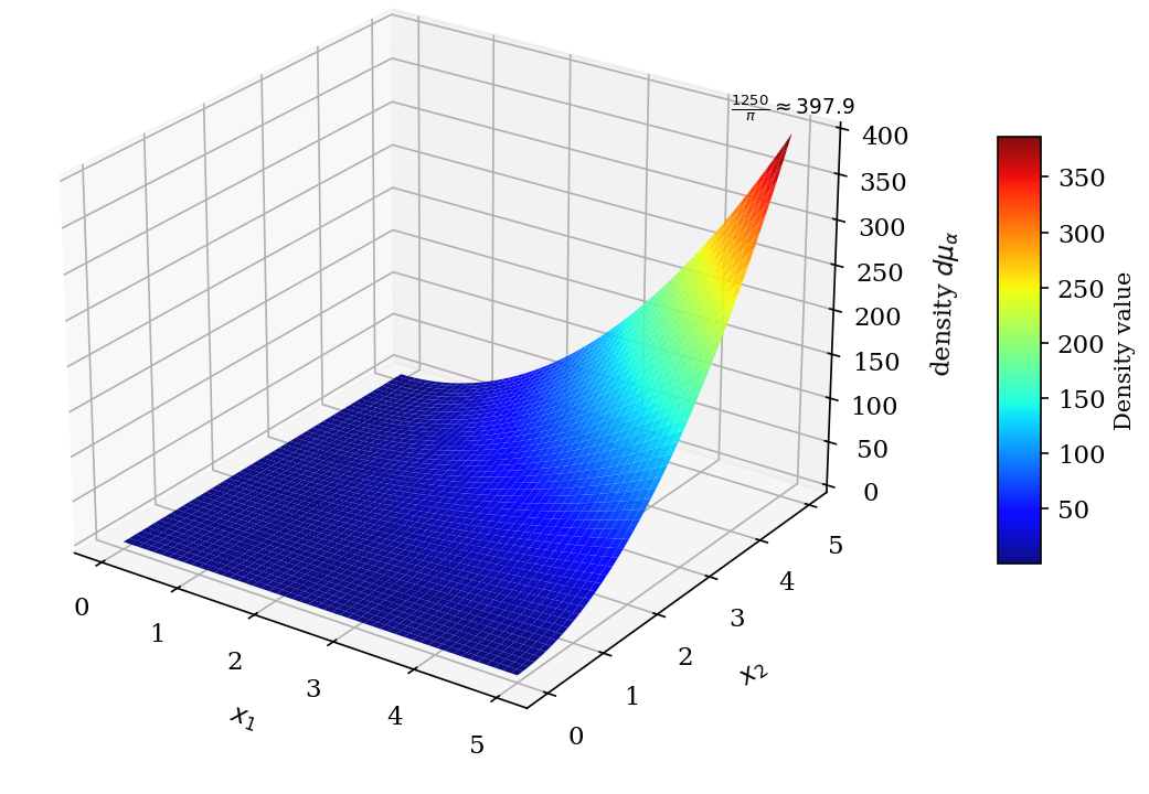
Figure 1 illustrates the density of this weighted measure, which grows rapidly away from the axes. This non-homogeneous geometry has a direct consequence for the scalogram: a signal concentrated near the axes will produce a systematically weaker response than a signal of equal \(L^{2}_{\alpha}(\mathbb{R}^{2}_{+} )\)-norm located farther from them.
The Fourier–Bessel wavelet considered in this work is the Mexican-hat-Bessel wavelet \[g(x_{1},x_{2})=\frac{12-x_{1}^{2}-x_{2}^{2}}{4\sqrt{3}}e^{-(x_{1}^{2}+x_{2}^{2})/4},\tag{22}\] with \(\|g\|_{L^{2}_{\alpha}(\mathbb{R}^{2}_{+})}=1\) and \(\omega_{g}=\frac{8}{3}\). The constant \(\|g\|_{L^{2}_{\alpha}(\mathbb{R}^{2}_{+})}=1\) is verified by direct computation using \[\int_{\mathbb{R}_+}x^{2k}e^{-x^{2}/2}\mbox{d}x=2^{k-1/2}\Gamma\bigl(k+\tfrac{1}{2}\bigr).\]
The admissibility condition \(\omega_{g}=\frac{8}{3}\) follows from the fact that \[\mathscr{F}_{\alpha}(g)(\lambda_{1},\lambda_{2})=(\lambda_{1}^{2}+\lambda_{2}^{2})e^{-(\lambda_{1}^{2}+\lambda_{2}^{2})},\] by substituting \(u=2a^{2}\lambda^{2}\) in the admissibility condition (4) and integrating over \(\mathbb{R}^{2}_{+}\) with respect to \(\mu_{\alpha}\). Both constants are independent of \(\lambda\) in accordance with condition (4).
The dominant analyzed frequency, obtained by maximizing \(\lambda^{2}e^{-\lambda^{2}}\) over \(\lambda^{2}=\lambda_{1}^{2}+\lambda_{2}^{2}\), is \(\lambda_{\max}=1\). For the dilated wavelet \(g_{a}(x_{1},x_{2})=a^{-6}g(\frac{x_{1}}{a},\frac{x_{2}}{a})\), the spectral profile becomes \(\mathscr{F}_{\alpha}(g_{a})(\lambda)=a^{2}(\lambda_{1}^{2}+\lambda_{2}^{2}) e^{-a^{2}(\lambda_{1}^{2}+\lambda_{2}^{2})}\), and the dominant frequency shifts to \(\lambda_{\max}(a)=\frac{1}{a}\). Decreasing \(a\) shifts the analysis toward higher frequencies and finer structures, while increasing \(a\) favors lower-frequency components.
To illustrate the influence of the analyzed signal on the wavelet transform and the scalogram, we consider two test signals with contrasting spectral characters:
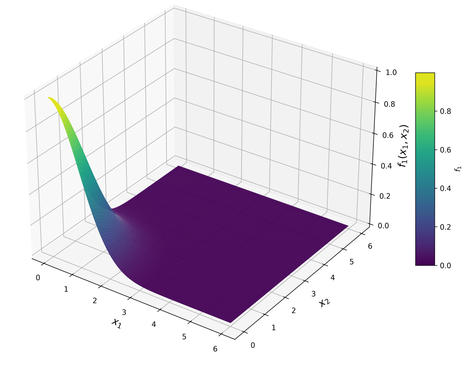
Signal 1: \(f_{1}(x_{1},x_{2})=e^{-(x_{1}^{2}+x_{2}^{2})/2}\), with a broad-band Fourier–Bessel spectrum concentrated near low frequencies (see Figure 2).
Signal 2: \(f_{2}(x_{1},x_{2}) =\cos(3x_{1})\cos(3x_{2})\,e^{-(x_{1}^{2}+x_{2}^{2})/8}\), whose Fourier–Bessel spectrum is concentrated near \(\lambda=3\), corresponding to the dominant scale \(a=1/3\) of the wavelet (see Figure 3).
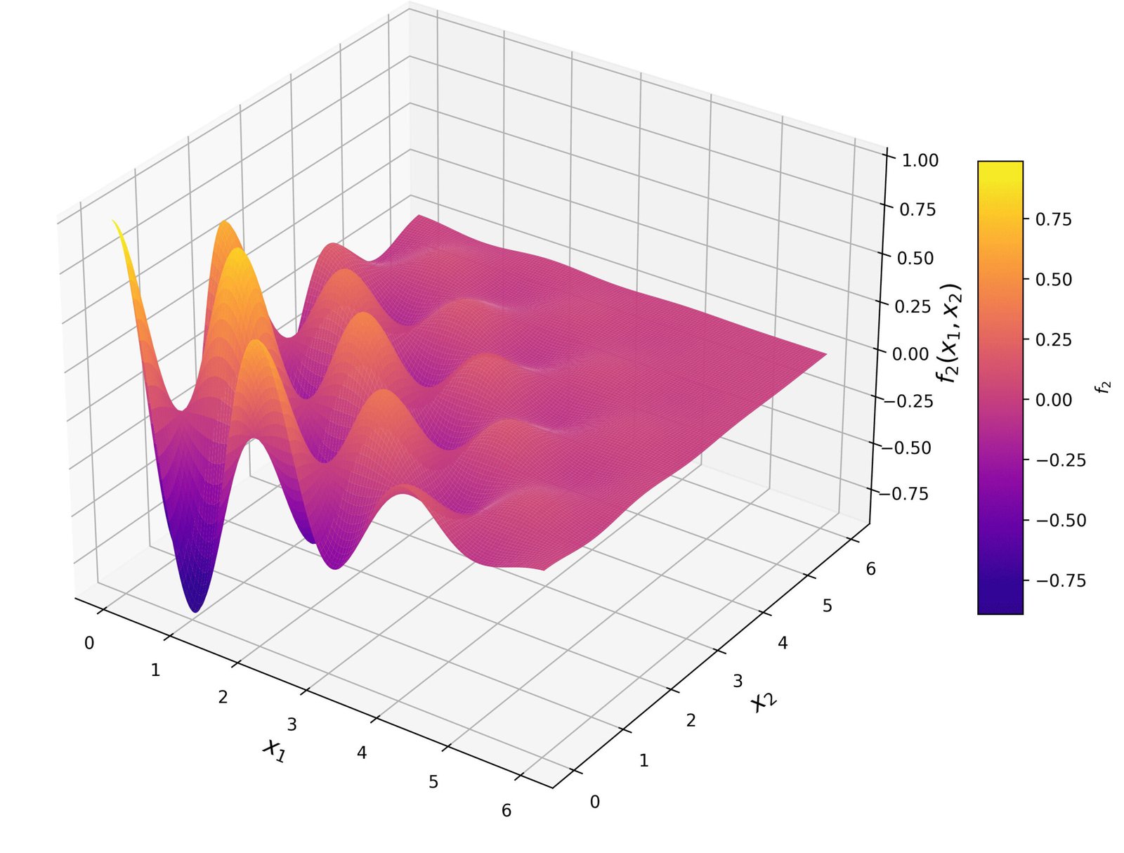
Both signals belong to \(L^{2}_{\alpha}(\mathbb{R}^{2}_{+})\). These two signals are chosen to represent the two extreme regimes of the signal-wavelet interaction: \(f_{1}\) yields a broad-band response while \(f_{2}\) produces a resonance near \(\lambda=3\), allowing a clear illustration of the diagnostic power of the scalogram.
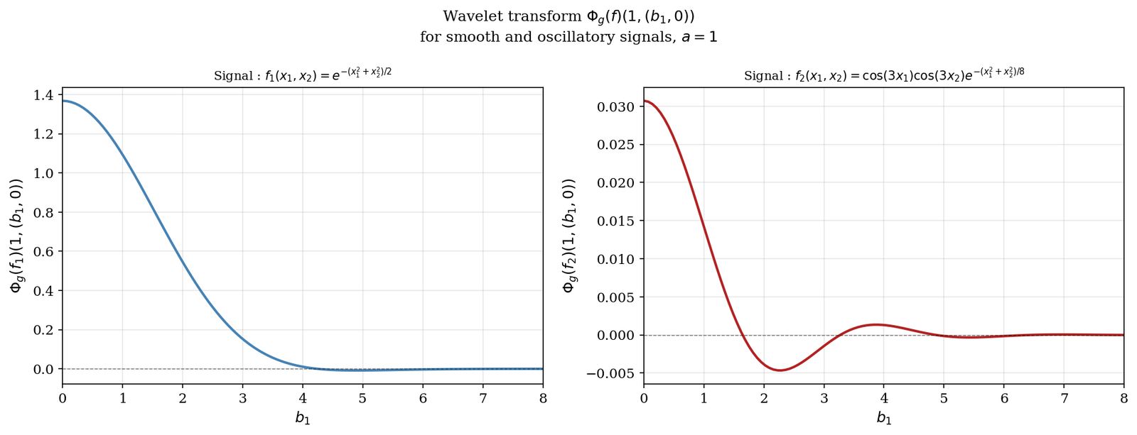
One of the principal differences between classical wavelets and Fourier–Bessel wavelets concerns the notion of translation. In the classical Euclidean framework, \(f(x)\mapsto f(x-b)\) preserves the shape of the wavelet. In contrast, the Fourier–Bessel framework involves the generalized translation operator \(\tau_{b}\) defined in (1). Applying \(\tau_{b}\) to \(g_{a}\) using representation (1) and form (22) yields \[\begin{aligned} g_{a,b}(x_{1},x_{2}) &=\left[1-\frac{|x|^{2}+|b|^{2}}{4a^{2}} +\frac{b_{1}x_{1}}{2a^{2}}\coth\!\left(\frac{b_{1}x_{1}}{2a^{2}}\right) +\frac{b_{2}x_{2}}{2a^{2}}\coth\!\left(\frac{b_{2}x_{2}}{2a^{2}}\right) \right]\\[4pt] &\quad\times \frac{4\,e^{-\frac{|x|^{2}+|b|^{2}}{4a^{2}}}\; \operatorname{sinch}\!\left(\frac{b_{1}x_{1}}{2a^{2}}\right)\; \operatorname{sinch}\!\left(\frac{b_{2}x_{2}}{2a^{2}}\right) }{\sqrt{3}\,a^{2}}, \end{aligned}\] where \(|x|^{2}=x_{1}^{2}+x_{2}^{2}\), \(|b|^{2}=b_{1}^{2}+b_{2}^{2}\), and \[\operatorname{sinch}(u) :=\begin{cases} \sinh(u)/u & u\neq 0,\\[2pt] 1 & u=0, \end{cases}\] is real-analytic on \(\mathbb{R}\), ensuring that \(g_{a,b}\) extends continuously to \(\mathbb{R}^{2}_{+}\) including the cases \(b_{i}=0\) or \(x_{i}=0\). The wavelet transform \[\Phi_{g}(f)(a,b)=\frac{2}{\pi}\int_{\mathbb{R}^{2}_{+}} f(x_{1},x_{2})\,g_{a,b}(x_{1},x_{2})\,x_{1}^{2}x_{2}^{2}\mbox{d}x_{1}\mbox{d}x_{2},\] is approximated by a composite Gauss–Legendre quadrature rule on \([0.02,10]^{2}\) with \(N_{q}=200\) nodes per direction. The scale parameter ranges over \(a\in\{0.5,\,0.75,\,1,\,1.5,\,2,\,3,\,4\}\) and the translation parameter over the grid \(b_{1},b_{2}\in\{0.1,\,0.2,\,\ldots,\,6.0\}\), see Figure 4.
For signal \(f_1\), the transform decays smoothly and monotonically as \(b_{1}\) increases, reflecting the globally concentrated low-frequency nature of \(f_{1}\). For signal \(f_2\), the transform exhibits rapid oscillations in \(b_{1}\), directly reflecting the oscillatory character of \(\cos(3\,\cdot\,)\) and its resonance with the wavelet at scale \(a=1\). Both behaviors are consistent with the Plancherel formula \(\omega_{g}^{-1}\|\Phi_{g}(f)\|^{2}_{L^{2}_{\alpha}(\mathbb{R}^*_+\times\mathbb{R}_+^2)} =\|f\|^{2}_{L^{2}_{\alpha}(\mathbb{R}_+^2)}\) holds for each signal regardless of the oscillatory pattern. The associated scalogram is defined by \(S_{g}(f)(a,b)=\frac{3}{2\pi^{2}}\,\bigl|\Phi_{g}(f)(a,b)\bigr|^{2}\). By (19), \(\|S_{g}(f)\|_{L^{1}_{\alpha}(\mathbb{R}^*_+\times\mathbb{R}_+^2)}=\|f\|^{2}_{L^{2}_{\alpha}(\mathbb{R}_+^2)}\), so the total energy of \(f\) is conserved across all scales and positions. Figure 5 presents the scalograms of both signals as functions of \((b_{1},b_{2})\in[0.1,6]^{2}\) at fixed scale \(a=1\).
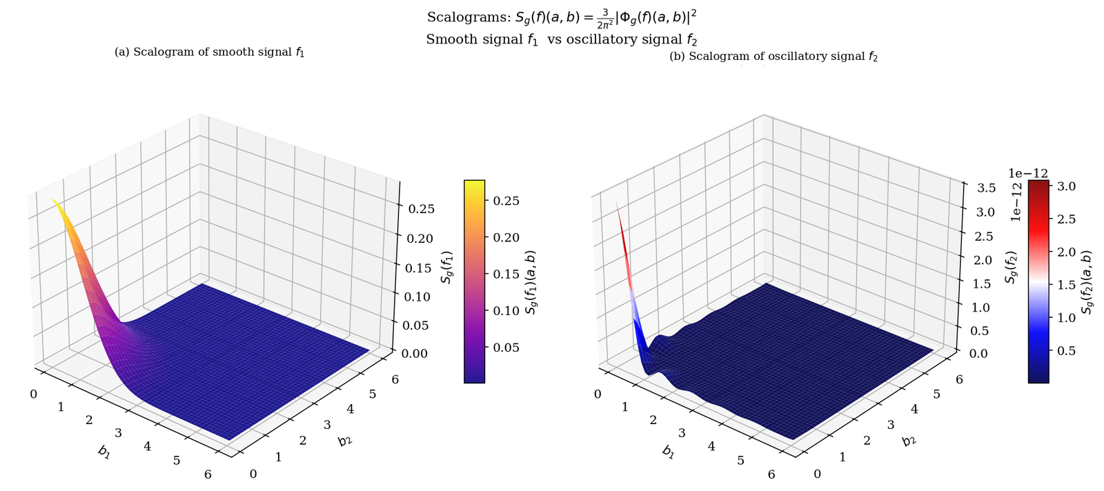
The scalogram of Signal \(f_1\) exhibits a single peak near \(b\approx(0.5,0.5)\), decaying smoothly, capturing the global energy envelope. The scalogram of Signal \(f_2\) reveals multiple oscillatory peaks with period \(2\pi/3\approx 2.09\), matching \(\cos(3\,\cdot)\). This resonance results from spectral overlap between \(\mathscr{F}_{\alpha}(g_{1})\) (peaked at \(\lambda=1\)) and \(\mathscr{F}_{\alpha}(f_{2})\) (peaked at \(\lambda=3\)); at \(a=1/3\) it would be maximal.
These results confirm that the scalogram is sensitive to the nature of the analyzed signal: smooth signals yield slowly varying, concentrated coefficients, while oscillatory signals generate modulated, frequency-rich representations. Moreover, the non-Euclidean geometry of the generalized translation \(\tau_{b}\) introduces a position dependent frequency sensitivity the shape of \(g_{a,b}\) deforms with \(b\) under the influence of the weight \(x_{1}^{2}x_{2}^{2}\) which is a purely Fourier–Bessel phenomenon with no counterpart in the classical Euclidean setting. Overall, these examples illustrate that the multidimensional Fourier–Bessel wavelet transform is particularly well adapted to the analysis of signals defined on weighted radial structures and non-Euclidean geometries.
In this paper, we have developed a comprehensive time-frequency analysis framework associated with the multidimensional Fourier–Bessel wavelet transform.
Summary of main results.
We summarize the obtained results as the following:
We established that the range of the transform \(\Phi_g\) is a reproducing kernel Hilbert space (RKHS) with explicit kernel \(W_g\) (Theorem 5). This provides a geometric framework for understanding the transform’s structure.
For a subset \(U \subset \mathbb{R}_+^{\ast} \times \mathbb{R}_+^d\) of finite \(\eta_\alpha\)-measure, we introduced the time-frequency operator \(\mathscr{L}_{g,U}\) and proved its boundedness (Theorem 8) and trace-class property (Theorem 9), with an explicit trace formula.
We defined Calderón–Toeplitz operators \(T_{g,U}\) in the Fourier–Bessel wavelet setting, showed their relation with \(\mathscr{L}_{g,U}\), and proved they are trace-class with a diagonalization in terms of the eigenfunctions of \(\mathscr{L}_{g,U}\) (Theorems 10, 11 and Remark 2).
In the context of scalogram analysis, we introduced the subspace scalogram \(\mbox{Scal}_g^V\) and proved that the optimal time-frequency concentration in \(U\) is achieved by the first \(N\) eigenfunctions of \(\mathscr{L}_{g,U}\) (Theorem 13). We also derived an error estimate for the accumulated scalogram (Theorem 14).
Numerical experiments in the case \(d=2\), \(\alpha=(\frac{1}{2},\frac{1}{2})\) illustrated the non-homogeneous geometry of the Fourier–Bessel framework and compared the behavior of Mexican-hat and Morlet-type wavelets.
Limitations.
The present work assumes that the analyzing wavelet \(g\) satisfies the admissibility condition (3.2) and that \(\|g\|_{L_\alpha^2}=1\). The case \(\alpha_k = -\frac{1}{2}\) is excluded due to the translation operator definition. Moreover, the numerical examples are limited to a specific signal and wavelet; a systematic study of the influence of parameters on the concentration properties remains to be done.
Future work.
Several directions can be pursued:
Higher dimensions. Extend the analysis to arbitrary dimension \(d\) with a detailed study of the dependence of the eigenvalues \(s_n(U)\) on the geometry of \(U\).
Adaptive wavelet selection. Determine the optimal wavelet \(g\) that maximizes the concentration of the first eigenfunctions for a given domain \(U\).
Applications. Apply the proposed scalogram analysis to real-world problems such as biomedical signal processing (ECG, EEG), vibration analysis, or ultrasound imaging, where the Fourier–Bessel framework is particularly relevant.
Uncertainty principles. Investigate the connection between the concentration estimates obtained here and the uncertainty principles for the Fourier–Bessel transform.
Numerical implementation. Develop an efficient numerical library for the multidimensional Fourier–Bessel wavelet transform, including fast algorithms for the translation operator and the eigenvalue decomposition of \(\mathscr{L}_{g,U}\).
In conclusion, this contribution provides a working basis for time-frequency analysis within the framework of Fourier–Bessel setting and opens the way to numerous applications in signal processing on weighted radial domains.
Conflicts of Interest: The authors declare no competing interests.
Data Availability: There is no data used in this manuscript.
Funding Information: This research did not receive funding.
Acknowledgments: The authors are deeply grateful to the referee for his constructive comments and valuable suggestions.