It is on record that rolling out COVID-19 vaccines has been one of the fastest for any vaccine production worldwide. Despite this prompt action taken to mitigate the transmission of COVID-19, the disease persists. One of the reasons for the persistence of the disease is that the vaccines do not confer immunity against the infections. Moreover, the virus-causing COVID-19 mutates, rendering the vaccines less effective on the new strains of the disease. This research addresses the multi-strains transmission dynamics and herd immunity threshold of the disease. Local stability analysis of the disease-free steady state reveals that the pandemic can be contained when the basic reproduction number, \(R_{0}\) is brought below unity. The results of numerical simulations also agree with the theoretical results. The herd immunity thresholds for some of the vaccines against COVID-19 were computed to guide the management of the disease. This model can be applied to any strain of the disease.
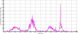
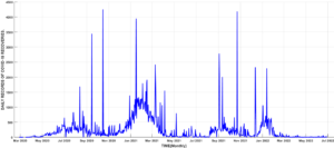
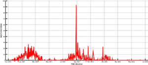
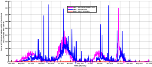
The spread of COVID-19 since its first Infection in Wuhan, China, has witnessed massive interventions by world leaders to get the pandemic under control [1,2]. Some of the interventions include media campaigns for the use of non-pharmaceutical measures such as the use of face masks, social distancing, isolation, lockdown, and handwashing, among others [3-5]. Efforts were also intensified towards the development of vaccines to curb the spread of the disease, leading to the rolling out of vaccines such as AstraZeneca, Moderna, etc. [6-9]. Despite these interventions, the disease persists because the vaccines developed so far can only reduce the infection rate and severity of the disease[10]. Hence, the disease still infects those who have been vaccinated. Another advantage of the vaccines is that the disease-induced death rate is reduced[11]. Another reason for the persistence of the disease is the fact that the virus causing the disease mutates, hence rendering the existing vaccines ineffective [12]. The mutation of the COVID-19 virus gives rise to different strains of the disease [12,13], hence the need to incorporate this in the modeling of the transmission dynamics of the disease. Many mathematical models of COVID-19 transmission have been used to predict the dynamics of this disease. Some models focus on non-pharmaceutical control measures for COVID-19, such as [3-5,14], and many more. Asymptomatic transmission of the disease has also been modeled by several researchers, including [15,16], and [17]. Since the discovery of COVID-19 vaccines, Scientists have examined the effects of such vaccines on the eradication of the disease [7,13]. Multiple strain transmission models have also been developed to study the transmission dynamics of the pandemic. In the current work, we intend to construct a multiple strains COVID-19 model incorporating vaccination to determine the herd immunity threshold for eradicating the disease. To our knowledge, this aspect has not been adequately addressed by researchers. The emergence of different strains of the disease has led to new waves of infections worldwide. Daily reported cases of infections in Nigeria shows clearly the distinct waves of infections in the country, as can be seen in Figure 1. The most severe waves of infections were witnessed in Nigeria between January and March 2021, December 2021, and February 2022. Daily recoveries were also recorded from the first case of the disease in the country in February 2020 [18] up to June 2022. This is depicted in Figure 2. However, you will notice some isolated high figures of recoveries for some days. These were due to accumulated recoveries that were not reported at the right time. Daily death records are represented in Figure 3. The one isolated case in this Figure was also accumulated records of deaths that were reported in one day. Figure 4, on the other hand, shows the daily records of new infections, recoveries, and deaths. It is clear from the figure that daily mortality from the disease in Nigeria is negligible compared to new infections and recoveries. Subsequent sections of this paper are organized as follows: Section 2 is dedicated to the model formulation to be followed by the local stability analysis of the disease-free equilibrium in section 3, while results and discussion will be the subject of section 4, and finally, the conclusion will come up in section 5.
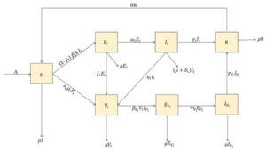
We construct a mathematical model focusing on the effects of vaccination in a multiple-strain transmission of COVID-19. This is divided into the following compartments: the susceptible individuals \(S(t)\), the exposed individuals \(E_{i}(t)\), the infected individuals \(I_{i}(t)\), the vaccinated individuals \(V_{i}(t)\), the exposed vaccinated individuals \(E_{V_{i}}(t)\), the infected vaccinated individuals \(I_{V_{i}}(t)\), and the removed/recovered individuals \(R(t)\), with total population given by \[N(t) = S(t) + E_{i}(t) + I_{i}(t) + V_{i}(t) + E_{V_{i}}(t) + I_{V_{i}}(t) + R(t) .\] The flow diagram of the transmission dynamics based on these compartments is shown in Figure 5. Following the flow diagram, the governing equations for the dynamics of the disease are given by \[\ dfrac{dS}{dt} = \Lambda-(1-\rho_{i})\beta_{i}SI_{i}-\lambda_{i}\rho_{i}V_{i}-\mu{S}+\theta{R} \\ \dfrac{dE_{i}}{dt} = (1-\rho_{i})\beta_{i}SI_{i} – \left(\omega_{i}+\xi_{i}+\mu\right)E_{i} \\ \dfrac{dI_{i}}{dt} = \omega_{i}{E_{i}} – \left(\gamma_{i}+\eta_{i}+\mu+\delta_{i}\right)I_{i}\\\dfrac{dV_{i}}{dt} = \left(\lambda_{i}\rho_{i}-\mu\right){V_{i}}+\xi_{i}{E_{i}}+\eta_{i}{I_{i}}-\beta_{V_{i}}{V_{i}}{I_{V_{i}}} \\\dfrac{dE_{V_{i}}}{dt} = \beta_{V_{i}}{V_{i}}{I_{V_{i}}} – \left(\omega_{V_{i}}+\mu\right)E_{V_{i}}\\ \dfrac{dI_{V_{i}}}{dt} = \omega_{V_{i}}{E_{V_{i}}} – \left(\gamma_{V_{i}}+\mu\right){I_{V_{i}}}\\ \dfrac{dR}{dt} = \gamma_{V_{i}}{I_{V_{i}}} +\gamma_{i}{I_{i}}-\left(\mu+\theta\right){R}, \tag{1}\] with the initial conditions \[S(0)>0, E_{i}(0)> 0, I_{i}(0)\geq 0, V_i(0)\geq 0,E_{V_{i}}\geq 0,I_{V_{i}}\geq 0, R(0)\geq 0.\] The parameter \(\Lambda\) is the recruitment rate of susceptible individuals, \(\beta_{i}\) and \(\beta_{V_{i}}\) are effective rates of Infection of susceptible individuals and vaccinated individuals, respectively, \(\delta_{i}\) is the disease induced death rate of the infectives, \(\omega_{i}\) and \(\omega_{V_{i}}\) are the rates at which the exposed and the exposed vaccinated individuals move into the infective compartment, \(\gamma_{i}\) and \(\gamma_{V_{i}}\) are the recovery rates of infected and vaccinated individuals respectively, \(\theta\) is the rate at which the recovered return to the susceptible class, \(\mu\) is the natural death rate of individuals, \(\eta_{i}\) is the rate at which the infected are vaccinated, \(\xi_{i}\) is the rate at which the exposed are vaccinated, \(\lambda_{i}\) is rate of progression from susceptible to the vaccinated, while \(0 < \rho_{i} < 1\) is the proportion of susceptible individuals who are vaccinated. All the parameters are positive and each of them is taken as a rate per day, while \(i\) represents the variant of the virus. The feasible region for the system (1) is given by \[\Psi =\left\{(S,E,I,V,E_{V},I_{V},R)\in {R_{+}^{7}}: S + E + I + E_{V}+ I_{V} + R \leq \dfrac{\Lambda}{\mu}\right\} ,\] which is bounded and positively invariant. The basic reproduction number \({\Re_{0}}\) of the model is obtained using the next-generation matrix procedure. Hence, we express the governing equations of the infected compartments as \[\dfrac{dX_{i}}{dt} = {F_{i}(X)}-{V_{i}}(X),\] where \(X\equiv [E_{i}, I_{i},E_{V_{i}},I_{V_{i}}]^{T}\equiv [x_{1}, x_{2}, x_{3}, x _{4}]^{T}\), then \(F = \left[\dfrac{\partial {f_{ij}}}{\partial{x_{i}}}\right]_{X_{0}}, V = \left[\dfrac{\partial {v_{ij}}}{\partial{x_{i}}}\right]_{X_{0}}, 1\leq i, j\leq {4},\) where \(X_{0} = \left(\dfrac{\Lambda}{\mu}, 0, 0, 0, 0, 0, 0 \right)^{T}\), \({F_{i}}\) are the new infections in compartment \(i\) and \(V_{i}\) are the rates of transfer of infections in and out of the compartments. To avoid any confusion, the largest eigenvalue of the next generation matrix \({FV^{-1}}\), is the basic reproduction number. From (1), we obtain \[\ F_{1} = \left(1-\rho_{i}\right)\beta_{i}SI_{i}\\ F_{2} = 0\\ F_{3} = \beta_{V_{i}}V_{i}I_{V_{i}}\\ F_{4} = 0, \tag{2}\] and \[\ V_{1} = \left(\omega_{i}+\xi_{i}+\mu\right)E_{i} \\ V_{2} = \left(\gamma_{i}+\eta_{i}+\mu+\delta_{i}\right)-\omega_{i}E_{i}\\ V_{3} = \left(\omega_{V_{i}}+\mu\right)E_{V_{i}}\\ V_{4} = \left(\gamma_{V_{i}}+\mu\right)I_{V_{i}}-\omega_{V_{i}}E_{V_{i}}, \tag{3}\] From (2) and (3), we obtain the Jacobian matrices evaluated at the disease-free equilibrium as \[F = \left(\begin{matrix} 0& \frac{(1-\rho_{i})\Lambda\beta_{i}}{\mu}& 0& 0\\ 0& 0& 0& 0\\ 0& 0& 0& 0\\ 0& 0& 0& 0\\ \end{matrix}\right)\] and \[V = \left(\begin{matrix} \omega_{i}+\xi_{i}+\mu& 0& 0& 0\\ -\omega_{i}& \gamma_{i}+\eta_{i}+\mu+\delta_{i}& 0& 0\\ 0& 0& \omega_{V_{i}}+\mu& 0\\ 0& 0& -\omega_{V_{i}}& \gamma_{V_{i}}+\mu\\ \end{matrix}\right)\] with\(\mid {V}\mid = (\mu+\omega_{i}+\xi_{i})(\gamma_{i}+\eta_{i}+\mu+\delta_{i})(\mu+\omega_{V_{i}})(\gamma_{V_{i}}+\mu).\) The inverse of the matrix V is obtained as \[V^{-1}=\left(\begin{matrix} \frac{1}{\mu+\omega_{i}+\xi_{i}}& 0& 0& 0\\ \frac{\omega_{i}}{(\mu+\omega_{i}+\xi_{i})(\gamma_{i}+\eta_{i}+\mu+\delta_{i})}& \frac{1}{\gamma_{i}+\eta_{i}+\mu+\delta_{i}} & 0& 0\\ 0& 0& \frac{1}{\mu_{i}+\omega_{i}}& 0\\ 0& 0& \frac{\omega_{V_{i}}}{(\mu+\omega_{V_{i}})(\gamma_{V_{i}+\mu})}& \frac{1}{\gamma_{v_{i}+\mu}} \end{matrix}\right).\] Hence, the next generation matrix \((FV^{-1}),\) is given by \[FV^{-1} = \left(\begin{matrix} \frac{(1-\rho_{i})\beta_{i}\Lambda\omega_{i}}{\mu(\mu+\omega_{i}+\xi_{i})(\gamma_{i})+\eta_{i}+\mu+\delta_{i})}& \frac{\Lambda(1-\rho_{i})\beta_{i}}{\mu(\gamma_{i}+\eta_{i}+\mu+\delta_{i})}& 0& 0\\ 0& 0& 0& 0\\ 0& 0& 0& 0\\ 0& 0& 0& 0\\ \end{matrix}\right)\tag{4}\]
with the eigenvalues \(\Lambda_{1} = \Lambda_{2} = \Lambda_{3} = 0\) and \(\Lambda_{4} = \frac{(1-\rho_{i})\beta_{i}\Lambda\omega_{i}}{\mu(\mu+\omega_{i}+\xi_{i})(\gamma_{i}+\eta_{i}+\mu+\delta_{i})}.\) Thus, the basic reproduction number, \(\Re_{0}\) is the spectral radius of the next generation matrix \((FV^{-1} ),\) given by
\[\ Re_{0}= \frac{(1-\rho_{i})\beta_{i}\Lambda\omega_{i}}{\mu(\mu+\omega_{i}+\xi_{i})(\gamma_{i}+\eta_{i}+\mu+\delta_{i})}. \tag{5}\] The baseline parameters obtained for the model are tabulated below:
| Parameter | Description | Estimated value |
| \(\Lambda\) | Recruitment rate of susceptible individuals. | \(0.0375\) [14] |
| \(\theta\) | Rate at which the recovered lose immunity | \(1.000\) assumed |
| \(\beta_i\) | Effective rate of infection of individuals | \(0.14\) estimated [19] |
| \(\mu\) | Natural death rate of individuals | \(0.015 \) [14] |
| \(\rho_i\) | Proportion of susceptible individuals who are vaccinated. | \(0.13\) assumed |
| \(\omega_i\) | The effective rate of exposed individuals. | \(0.12 \) assumed |
| \(omega_v_i)\ | The rate of exposure of vaccinated individuals. | \(0.16\) assumed |
| \(\gamma_i\) | Recovery rate of infected individuals. | \(0.27\) estimated [20] |
| \(\delta_i\) | Disease induced death rate of the infectives. | \(0.021\) estimated [21] |
| \(\xi_i\) | Rate at which the exposed are vaccinated. | \(0.10\) assumed |
| \(\eta_i\) | Rate at which the infected are vaccinated. | \(0.20 \) assumed |
| \(beta_v_i)\ | Effective rate of infection of vaccinated individuals. | \(0.16\) assumed |
| \(gamma_v_i)\ | Recovery rate of vaccinated individuals | \(1.000 \) assumed |
| \(\lambda_i\) | rate of progression from susceptible to the vaccinated. | \(0.06\) assumed |
Definition 1. The normalised sensitivity index \(\gamma^{R}_{\lambda}\) of the variable \(R(\lambda)\) is defined by \[\gamma^{R}_{\lambda} =\dfrac{\partial R}{\partial \lambda} \times \frac{\lambda}{R}, \tag{6}\]
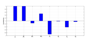
Using (6), we obtain the sensitivity indices of the various parameters contained in the basic reproduction number \(\Re_{0}\) as depicted in Table 2, based on the baseline parameter values in Table 1
| Parameter | Sensitivity index |
| \( \Lambda\) | \(1.000\) |
| \(\beta_i\) | \(1.000\) |
| \(\rho_i\) | \(-0.1494\) |
| \(\omega_i\) | \(0.4894\) |
| \( \gamma_i\) | \( -0.9029\) |
| \(\delta_i\) | \( 0.023\) |
| \(\xi_i\) | \(- 0.4255\) |
| \(\eta_i\) | \( -0.0564\) |
The essence of vaccination against any infectious disease is to protect the population from Infection and eventually bring the disease to an end. To eradicate the disease through vaccination, a certain threshold must be targeted. This threshold is referred to as the herd immunity threshold. Herd immunity is defined as the percentage of the susceptible population that must be vaccinated to stop disease transmission in that population. It can be expressed in terms of the basic reproduction number \(\Re_{0}\) as \(H_{im}= 100\left(1-\frac{1}{\Re_{0}}\right)\%\) for a vaccine that is \(100\%\) efficient. However, for an imperfect vaccine with efficacy \(V_{e},\) the threshold is expressed as \(H_{im}= \frac{100}{V_e}\left(1-\frac{1}{\Re_{0}}\right)\%.\) When \(V_{e}< 1- \frac{1}{\Re_{0}}\), the disease becomes impossible to eradicate even if the whole population is vaccinated (Fine, et al., 2011). The expression gives the herd immunity threshold for this model \[H_{im} = 1- \frac{\mu(\mu +\omega_{i} +\xi_{i})(\gamma_{i} + \eta_{i} + \mu +\delta_{i})}{\Lambda(1-\rho_{i})\beta_{i}\omega_{i}}.\] For the parameter values in Table \(1,\) \(\Re_{0}= 1.234\) and the corresponding herd immunity threshold for COVID-19 vaccines such as Moderna and Johnson and Johnson is \(H_{im} = 20.176\%.\) This means Nigeria must vaccinate about \(20\%\) of its population to eradicate COVID-19. However, with AstraZeneca with an efficiency of \(72\%,\) the herd immunity threshold is \(H_{im} = 26.341\%\), the country needs to vaccinate at least \(26\%\) of the population to get the disease under control.
Here, we examine the local stability of the disease-free equilibrium (DFE) in relation to the basic reproduction number, \(\Re_{0}\). The disease-free equilibrium is defined as the point at which no disease is present in the population, which occurs when \(E_{i} = I_{i} = E_{V_{i}} = I_{V_{i}} = R = 0.\)
We evaluate the Jacobian matrix at the DFE, denoted as \(\left(\frac{\Lambda}{\mu}, 0, 0, 0, 0, 0, 0\right)\), which yields:
\[J_{E_{0}} = \begin{pmatrix} -\mu & 0 & -\frac{\Lambda(1-\rho_{i})\beta_{i}}{-\lambda_{i}\rho_{i}} & 0 & 0 & 0 & 0 \\ 0 & -(\omega_{i} + \xi_{i} + \mu) & \frac{\Lambda(1-\rho_{i})\beta_{i}}{\mu} & 0 & 0 & 0 & 0 \\ 0 & \omega_{i} & -(\gamma_{i} + \eta_{i} + \mu + \delta_{i}) & 0 & 0 & 0 & 0 \\ 0 & \xi_{i} & \eta_{i} & \lambda_{i\rho_{i}}-\mu & 0 & 0 & 0 \\ 0 & 0 & 0 & 0 & -(\mu+\omega_{V_{i}}) & 0 & 0 \\ 0 & 0 & 0 & 0 & \omega_{V_{i}} & -(\gamma_{v_{i}}+\mu) & 0 \\ 0 & 0 & \gamma_{i} & 0 & 0 & \gamma_{V_{i}} & -(\mu+\theta) \\ \end{pmatrix}\tag{7}\]
This matrix has the following eigenvalues: \(\Lambda_{1} = -\mu\), \(\Lambda_{2} = -(\mu + \theta)\), \(\Lambda_{3} = \lambda_{i}\rho_{i} – \mu\), \(\Lambda_{4} = – (\gamma_{V_{i}}+\mu)\), and \(\Lambda_{5} = -(\mu+ \omega_{V_{i}})\).
The remaining eigenvalues can be obtained from the sub-matrix:
\[J_{2} = \begin{pmatrix} – (\omega_{i} + \xi_{i} + \mu) & \frac{\Lambda(1-\rho_{i})\beta_{i}}{\mu} \\ \omega_{i} & -(\gamma_{i} + \eta_{i} + \mu + \delta_{i}) \\ \end{pmatrix}\]
The matrix (7) has the characteristic polynomial:
\[\lambda^{2} + (2\mu + \gamma_{i} + \omega_{i} + \xi_{i} + \eta_{i} + \delta_{i})\lambda + (\mu + \omega_{i} + \xi_{i})(\gamma_{i} + \eta_{i} + \mu + \delta_{i}) – \frac{\Lambda(1-\rho_{i})\beta_{i}\omega_{i}}{\mu} = 0\]
Which can be simplified to:
\[\frac{1}{(\mu + \omega_{i} + \xi_{i})(\gamma_{i} + \eta_{i} + \mu + \delta_{i})}\lambda + \frac{2\mu + \gamma_{i} + \eta_{i} + \omega_{i} + \xi_{i} + \delta_{i}}{(\mu + \omega_{i} + \xi_{i})(\gamma_{i} + \eta_{i} + \mu + \delta_{i})}\lambda + 1 – \Re_{0} = 0.\]
This equation can be rewritten as:
\[a_{0}\lambda^{2} + a_{1}\lambda + a_{2} = 0, \tag{8}\]
Where \[a_{0} = \frac{1}{(\mu + \omega_{i} + \xi_{i})(\gamma_{i} + \eta_{i} + \mu+\delta_{i})} > 0,\]
\[a_{1} = \frac{2\mu +\gamma_{i} + \eta_{i} + \omega_{i} + \xi_{i} + \delta_{i}}{(\mu + \omega_{i} + \xi_{i})(\gamma_{i} + \eta_{i} + \mu + \delta_{i})} > 0,\]
and
\[a_{2} = 1 – \Re_{0}.\]
For the stability of the DFE, it is required that \(1 – \Re_{0} > 0\), leading to the condition \(\Re_{0} < 1\) and \(\lambda_{i}\rho_{i} < \mu\).
Hence, we conclude the following result:
Theorem 1. The disease-free equilibrium (DFE) of the model (1) is locally asymptotically stable for \(\Re_{0} < 1\) and \(\lambda_{i}\rho_{i} < \mu\), and unstable otherwise.
A model for the transmission dynamics of multi-strain COVID-19 infections with individual vaccination has been developed. Theoretical analysis of critical factors in disease management, including the basic reproduction number and the disease-free equilibrium, has been conducted. The disease-free equilibrium has been determined to be locally asymptotically stable when the basic reproduction number is less than unity (\(\Re_{0} < 1\)), subject to a minimum vaccination threshold within the population. The various parameters contributing to the basic reproduction number have been characterized by their sensitivity indices, as presented in Table 2.
Normalized sensitivity indices have been employed to identify parameters with a greater impact on disease transmission. These sensitivity indices can be positive or negative. The parameter with the highest positive (or negative) sensitivity index is the one most (or least) sensitive to \(\Re_{0}\), and thus, to disease transmission. Figure 6 visualizes the magnitudes of these sensitivity indices.
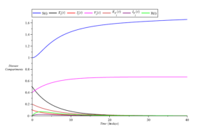
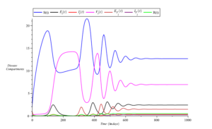
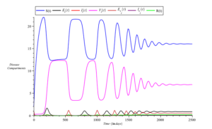
Simulations of the model equations were also conducted based on the parameter values in Table 1. The results are presented in Figures 7,8,9 and 10. The simulations reveal that infections decrease over time with reduced exposure to infection, as illustrated in Figure 7.
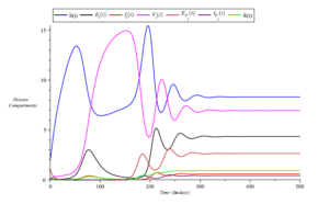
However, an increase in the recruitment rate of individuals (\(\Lambda = 0.375\)) results in a prolonged persistence of the disease, as observed in Figure 8. Figure 9 demonstrates that infections slow down with an increase in the proportion of vaccinated individuals (increasing from \(\rho_{i} = 0.13\) to \(\rho_{i} = 0.43\)).
Furthermore, Figure 10 highlights the fact that a further increase in the proportion of vaccinated individuals leads to a reduction in infections as well as exposure to the disease.
A multi-strains transmission dynamics of COVID-19 have been constructed and analyzed. The theoretical analysis, as well as numerical simulations, show that the disease can be contained when \(R_{0}<1\) and when more people are vaccinated. Herd immunity thresholds for the commonly used COVID-19 vaccines in Nigeria were also computed to guide policymakers.
Peirlinck, M., Linka, K., Sahli Costabal, F., & Kuhl, E. (2020). Outbreak dynamics of COVID-19 in China and the United States. Biomechanics and modeling in mechanobiology, 19(6), 2179-2193.
Ngonghala, C. N., Iboi, E., Eikenberry, S., Scotch, M., MacIntyre, C. R., Bonds, M. H., & Gumel, A. B. (2020). Mathematical assessment of the impact of non-pharmaceutical interventions on curtailing the 2019 novel Coronavirus. Mathematical biosciences, 325, Article, 108364.
Teklu, S. W. (2022). Mathematical analysis of the transmission dynamics of COVID-19 infection in the presence of intervention strategies. Journal of Biology Dynamics, 16(1), 640-664.
Adedire, O., & Ndam, J. N. (2021). A model of dual latency compartments for the transmission dynamics of COVID-19 in Oyo State, Nigeria. Engineering and Applied Sciences Letters, 4, 1-13.
Bok, K., Sitar, S., Graham, B. S., & Mascola, J. R. (2021). Accelerated COVID-19 vaccine development: Milestones, lessons, and prospects. Immunity, 54, 1636-1651.
MacIntyre, C. R., Costantino, K., & Trent, M. (2022). Modelling of COVID-19 vaccination strategies and herd immunity in scenarios of limited and full vaccine supply in NSW, Australia. Vaccine, 40, 2506-20513.
Negi, S. S., Rana, P. S., Sharma, N., & Khatri, M. S. (2022). A Novel SEIAHR compartment model for assessing the impact of vaccination, intervention policies, and quarantine on the COVID-19 pandemic: A case study of most affected countries Brazil, India, Italy, and USA. Computational and Applied Mathematics, 41, Article, 305.
Kashte, S., Gulbake, A., El-Amin III, S. F., & Gupta, A. (2021). COVID-19 Vaccines: Rapid development, implications, challenges, and future prospects. Human Cell, 34, 711-733.
Singh, C., Naik, B. N., Pandey, S., Biswas, B., Pati, B. K., Verma, M., & Singh, P. K. (2021). Effectiveness of COVID-19 vaccine in preventing Infection and disease severity: A case-control study from Eastern State of India. Epidemiology and Infection, 149, e224, 1-9.
Stepanova, M., Lam, B., Younossi, E., Felix, S., Ziayee, M., et al. (2022). The impact of variants and vaccination on the mortality and resource utilization of hospitalized patients with COVID-19. BMC Infectious Diseases, 22, Article, 702.
Sanz-Leon, P., Hamilton, L. H. W., Raison, S. J., Pan, A. J. X., Stevenson, N. J., Stuart, R. M., Abeysuriya, R. G., Kerr, C. C., Lambert, S. B., & Roberts, J. A. (2022). Modelling herd immunity requirement in Queensland: Impact of vaccination effectiveness, hesitancy, and variants of SARS-COV-2. Philosophical Transactions of the Royal Society A, 380, 20210311.
Massard, M., Eftimie, R., Perasso, A.,& Saussereau, B. (2022). A Multi-Strain epidemic model for COVID-19 with injected and asymptomatic cases: Application to French data. Journal of Theoretical Biology, Article, 545.
Ndam, J. N. (2020). Modelling the impacts of lockdown and isolation on the eradication of COVID-19. Biomath, 9, Article, 2009107.
Anguelov, R., Banaisiak, J., Bright, C., Lubuma, J., & Ouifki, R. (2020). The big unknown: The asymptomatic spread of COVID-19. Biomath, 9, Article, 2005103.
Ndam, J. N. (2021). Mathematical modelling of the dynamics of COVID-19 pandemic. Asia-Pacific Journal of Mathematics, 8.
Sharma, S., Volpert, V., & Barnerjee, M. (2020). Extended SEIQR type model for COVID-19 epidemic and data analysis. Mathematical Biosciences and Engineering, 17(6), 7562-7604.
Nigeria Centre for Disease Control (NCDC). (2020). COVID-19 outbreak in Nigeria Situation Report number 001.
Mizumoto, K., Kagaya, K., Zarebski, A., & Chowell, G. (2020). Estimating the asymptomatic proportion of coronavirus disease 2019 (COVID-19) cases on board the Diamond Princess cruise ship, Yokohama, Japan, 2020. Eurosurveillance, 25(10), Article, 2000180.
Nigeria Centre for Disease Control (NCDC). (2020). COVID-19 Situation Report 79, March 18.
Nigeria Centre for Disease Control (NCDC). (2020). COVID-19 Situation Report 173, August 19.