
Globally, 39.9 million [36.1–44.6 million] people lived with human immunodeficiency virus (HIV) at the end of 2023. An estimated 0.6% [0.6%–0.7%] of adults aged 15–49 years worldwide live with HIV, although the burden of the epidemic still varies considerably between countries and regions [1].
HIV damages your immune system by destroying a type of white blood cell that helps your body fight infections. This puts you at risk for other infections and diseases. AIDS stands for acquired immunodeficiency syndrome. It is the final stage of HIV infection. It occurs when the body’s immune system is severely damaged by the virus. Not all people with HIV develop AIDS. HIV is spread through certain bodily fluids from a person with HIV through unprotected vaginal or anal sex with a person who has HIV. It is also spread by sharing needles for drug use, through contact with the blood of a person who has HIV, from mother to fetus during pregnancy, and from mother to baby during birth or breastfeeding. There is no cure for HIV infection, but it can be treated with medications known as antiretroviral therapy [2].
Syphilis is a sexually transmitted infection caused by the Treponema pallidum bacterium. Syphilis is a curable bacterial infection, but if left untreated, especially in its later stages, it can lead to severe complications and even death. Acquired syphilis is transmitted by sexual contact, while congenital syphilis occurs when a mother infected with syphilis transmits the infection to her fetus during pregnancy [3].
In 2022, the World Health Organization (WHO) estimated that 8 million adults aged 15–49 years acquired syphilis worldwide. In 2022, the WHO estimated that 700,000 cases of congenital syphilis occurred worldwide [4].
In the same sexual contact, an individual can be infected with both infections. People with untreated syphilis are estimated to be 2 to 5 times more likely to acquire HIV during unprotected sexual contact due to broken epithelial barriers, immune cell activation, and recruitment at lesion sites. HIV infection can alter the natural course of syphilis (for example, faster progression, atypical presentations), increase treponemal load in bodily fluids, potentially increasing the risk of transmission and delay the healing of syphilitic sores, prolonging the infectious period. Syphilis is treated the same way in HIV-positive patients as in HIV-negative ones with the use of antibiotics, but with increased vigilance for complications, slower response to therapy, and higher risk of relapse or neurosyphilis [3, 5].
Pre-exposure prophylaxis (PrEP) is a highly effective strategy for HIV prevention. It reduces the risk of acquiring HIV through sexual contact by approximately 99% and through injection drug use by at least 74% [6]. In 2023, more than 3.5 million people worldwide had used PrEP for HIV prevention at least once, according to the World Health Organization [7]. Although this represents an increase from the 2.6 million users reported in 2022, uptake remains far below the global target of 21 million users by 2025 set by UNAIDS [8].
This raises important questions: Does PrEP implementation only impact HIV? How might it influence syphilis? Beyond preventing HIV infection, PrEP serves as a diagnostic gateway for other sexually transmitted infections (STIs). Individuals initiating or maintaining PrEP are typically advised to attend regular follow-up visits, usually every three months, that include screening for HIV, syphilis, gonorrhea, chlamydia, and sometimes hepatitis. This structured monitoring enables early detection and treatment of STIs that might otherwise remain asymptomatic or undiagnosed, thereby improving individual health outcomes and reducing community transmission [9– 11].
Due to the impact that syphilis and HIV-syphilis coinfection have on health systems worldwide, mathematical models have been developed in recent years for its study [12– 15]. Olopade et al. [12] presented a multiphase treatment model of syphilis to study its impact on the spread and control of infection, and showed that the best strategy to alleviate the disease burden is to reduce contact rates and increase treatment rates for people with secondary and primary syphilis. Chukwul et al. [13] proposed a mathematical model for syphilis transmission dynamics in the men who have sex with men (MSM) population that incorporates high/low risk transmission classes, and from their results they suggested that increasing syphilis treatment rates and reducing high/low risk infection rates are essential to control the spread of syphilis in the MSM population. Wang et al. [14] introduced and studied an epidemic model of HIV-syphilis coinfection and, using data of syphilis cases and HIV cases from the US, observed competition between both diseases and concluded that treatment of primary syphilis is more important to mitigate the transmission of syphilis, but could lead to an increase in HIV cases. David et al. [15] developed a mathematical model to study the co-interaction of HIV infection and syphilis among gay, bisexual, and other men who have sex with men (MSM). Their results showed that both diseases disappear or coexist when their reproduction number is less than or greater than one, HIV infection negatively impacts the prevalence of syphilis and vice versa, and one possibility of reducing HIV-syphilis coinfection among MSM is to increase the rates of testing and treatment for syphilis and HIV infection and to reduce the rate at which HIV-infected individuals abandon treatment.
Mathematical models studying the impact of PrEP have been developed since its implementation [16– 21]. For example, Kim et al. [16] constructed a mathematical model of HIV infection among men who have sex with men (MSM) in South Korea, and simulated the effects of early antiretroviral therapy (ART), early diagnosis, PrEP, and combined interventions on the incidence and prevalence of HIV/AIDS. Moya et al. [17] presented a mathematical model for studying the influence of PrEP and post-exposure prophylaxis (PEP) in the presence of undiagnosed and undetectable cases and tested the positive impact of these preventive methods on the diagnosis of new cases. Research using fractional order derivatives in the Capputo sense for the study of PrEP is presented by the authors in [18], and analogous results were obtained for this technique. Silva and Torres [19] proposed an epidemiological model for HIV/AIDS transmission that includes PrEP and calibrated the model with cumulative cases of HIV infection and AIDS recorded in Cape Verde from 1987 to 2014 and showed that PrEP significantly reduces HIV transmission. Omondi et al. [20] presented a mathematical model stratified by sex and sexual preference that includes PrEP, and the results shown that the introduction of PrEP reduces the spread of HIV.
Several studies have examined the relationship between HIV pre-exposure prophylaxis (PrEP) and syphilis transmission dynamics using mathematical modeling and epidemiological simulations. Pedrosa et al. [22] investigated the incidence and risk factors of acquired syphilis among HIV PrEP users in Brazil using a retrospective cohort design and multivariate analysis. They reported 19.1 cases per 100 person-years, identifying risk factors such as prior syphilis, irregular condom use, transactional sex, and recreational drug use, while female gender and certain racial groups were protective. The study highlights the importance of monitoring PrEP users with targeted prevention strategies and regular syphilis screening. Nguyen et al. [23] examined the association between sociodemographic factors, HBV and HCV infection, and syphilis among HIV PrEP users in Vietnam using a cross-sectional survey and logistic regression analysis. They found that male gender, being employed, and HBV infection were significantly associated with higher syphilis risk. The study underscores the need for targeted STI prevention and monitoring strategies within PrEP programs. Mendoça et al. [24] conducted an ecological study in Brazilian state capitals from 2018 to 2022 to examine the association between HIV PrEP administration, STI incidence, and socioeconomic indicators. They found that PrEP use was significantly correlated with syphilis and viral hepatitis incidences, as well as with social determinants such as illiteracy, income, and sanitation, highlighting regional disparities. The study emphasizes the importance of integrating social determinants into PrEP programs to improve access and reduce STI risk in vulnerable populations.
This study examines the impact of PrEP on HIV and syphilis epidemics through a mathematical model that captures their transmission and coinfection dynamics, with a focus on changes in infection rates and diagnostic outcomes associated with PrEP use. The model considers only sexual transmission, as it is the primary route for both HIV and syphilis, and because individuals seeking PrEP typically aim to reduce HIV risk through safer sexual practices. Novel aspects of the model include the inclusion of coinfection in risky sexual contact and the consideration of different forms of diagnosis, particularly through the PrEP program.
The structure of this article is as follows. §2 introduces the mathematical model and establishes its basic qualitative properties. §3 is dedicated to the analysis of the syphilis-only submodel, with and without the implementation of PrEP. §4 explores the impact of PrEP within the HIV–syphilis coinfection model. In §5, a global stability study of parameters relevant to the model dynamics is performed, as well as an exploration of the basic reproduction numbers and the HIV–syphilis coinfection model. Finally, §6 presents the main conclusions and discusses the implications of the results.
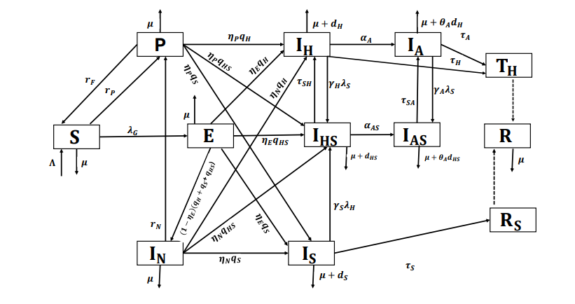
The model has twelve compartments: susceptibles (\(S\)), exposed (\(E\)), PrEP users (\(P\)), Individuals infected with HIV, syphilis, or undiagnosed HIV and syphilis coinfected individuals, either because they are not interested or because they are unaware of their status (\(I_{N}\)), Individuals mono-infected with HIV (\(I_{H}\)), Individuals mono-infected with HIV in AIDS stage (\(I_{A}\)), Individuals mono-infected with syphilis (\(I_{S}\)), HIV and syphilis co-infected individuals (\(I_{HS}\)), HIV and syphilis co-infected individuals in AIDS stage (\(I_{AS}\)), successfully treated for HIV (\(T_{H}\)), successfully treated and recovered from syphilis (\(R_{S}\)), and the individuals successfully treated for monoinfections or coinfections (\(R\)).
This study focuses solely on the sexual transmission of HIV and syphilis, as the main goal is to evaluate the impact of PrEP. Individuals seeking PrEP are typically sexually active and concerned with HIV prevention. Accordingly, the model’s dynamics are designed to reflect the behavior of a sexually active population.
The compartment \(I_{N}\) includes individuals who may be infected with HIV, syphilis, or coinfected with both, and who are distinguished in the transmission dynamics by modification parameters and by their diagnosis status.
As a novel contribution to the model, we incorporate the possibility of exposure to HIV, syphilis, or both (coinfection) during a single risk contact. Consequently, the exposed compartment (\(E\)) includes individuals who have been exposed to HIV, syphilis, or both infections. Upon becoming aware of their infection status, individuals transition from this compartment to the appropriate compartments: HIV infection (\(I_{H}\)), syphilis infection (\(I_{S}\)), or coinfection (\(I_{HS}\)). Those who remain undiagnosed or unaware of their infection status are directed to the compartment of undiagnosed infected individuals (\(I_{N}\)).
The recruitment rate is denoted by \(\Lambda\), representing the rate at which individuals become sexually active. We define the natural death rate as \(\mu\), which is assumed to be the same across all compartments. The disease-induced mortality rates for HIV, syphilis, and HIV-syphilis coinfection are represented by \(d_{H}\), \(d_{S}\), and \(d_{HS}\), respectively. For individuals with undiagnosed infections, we assume that disease-related death occurs only after diagnosis. The modification parameter \(\theta_{A}\) adjusts the mortality rates induced by HIV and HIV-syphilis coinfection in cases of AIDS.
The transmission rate for syphilis is \[\lambda_{S}= \dfrac{\beta_{S}(I_{S}+l_{S}(I_{HS}+I_{AS}+l_{NC}I_{N})+ l_{NS}I_{N})}{N}, \tag{1}\] for HIV is: \[\lambda_{H}= \dfrac{\beta_{H}(I_{H}+I_{A}+l_{H}(I_{HS}+I_{AS}+ l_{NC}I_{N})+l_{NH}I_{N})}{N}, \tag{2}\] and in sexual contact where the individual is exposed to both, the coinfection rate is: \[\lambda_{HS}= \dfrac{ \beta_{HS}(I_{HS}+I_{AS}+ l_{NC}I_{N})}{N}, \tag{3}\] where \(N(t)= S(t)+E(t)+P(t)+I_{N}(t)+I_{S}(t)+I_{H}(t)+I_{A}(t)+I_{HS}(t)+I_{AS}(t)+R(t)\) is the total population and \(\beta_{S}\), \(\beta_{H}\) and \(\beta_{HS}\) are the effective contact rates for syphilis, HIV, and HIV-syphilis coinfection, respectively. The modification parameters \(l_{S}\) and \(l_{H}\), where \(l_{S}, l_{H} > 1\), represent the increased infectivity for syphilis and HIV, respectively, in individuals coinfected with both infections, which exceeds that of individuals with a single infection. The parameters \(l_{NS}\), \(l_{NH}\), and \(l_{NC}\) denote the proportions of individuals with syphilis, HIV, and HIV-syphilis coinfection among the undiagnosed infected population.
The parameters \(\gamma_{H}\), \(\gamma_{A}\) and \(\gamma_{S}\) are associated with the enhancement of infectivity in HIV cases toward syphilis and vice versa, and we assume that \(\gamma_{H}, \gamma_{A},\gamma_{S}>1\).
An important feature of the model is that individuals in compartment P, while enrolled in the program, are protected against HIV but not against syphilis, and therefore can become infected with syphilis.
We define the general transmission rate, which means an individual can contract syphilis, HIV, or both, through sexual contact, as
\[\begin{aligned} \lambda_G = \lambda_H + \lambda_S + \lambda_{HS} =& \frac{I_N \left( \beta_S\,l_{N S} + \beta_H\, l_{N H} + \beta_{HS}\, l_{N C} \right)}{N}\nonumber \\ &+ \frac{\beta_S I_S + \beta_H (I_H + I_A) + (I_{HS} + I_{AS})(l_S \beta_S + l_H \beta_H + \beta_{HS})}{N}. \end{aligned} \tag{4}\]
The parameters \(r_{P}\) and \(r_{F}\) represent the rate at which individuals seek to enroll in the PrEP program and the rate of PrEP discontinuation or failure (i.e., the rate at which individuals leave the program for various reasons), respectively. Individuals infected with HIV, syphilis, or HIV–syphilis coinfection who are undiagnosed or unaware of their infection status may attempt to join the PrEP program at rate \(r_{N}\). Thus, the program can contribute to new diagnoses.
In constructing the model, we consider two pathways for diagnosing cases: following a sexual risk encounter (either immediately or some time afterward) and during the attempt to enroll in the PrEP program. The parameter \(\eta_{E}\) defines the diagnosis rate following a risk exposure, and in conjunction with \(q_{H}\), \(q_{S}\), and \(q_{HS}\), determines whether the diagnosis corresponds to HIV, syphilis, or coinfection. This is a key element, as early diagnosis helps control transmission and prevent clinical complications. However, if diagnosis does not occur—either because the individual avoids it or is unaware of the exposure—they remain in the compartment of undiagnosed infected individuals.
We therefore define \(\eta_{P}\) as the diagnosis rate for infected individuals who are undiagnosed or unaware of their status when attempting to access the PrEP program. We assume that HIV and syphilis testing is performed as a prerequisite for program entry.
Individuals in compartment \(I_{N}\) remain there until they either attempt to access the PrEP program or receive a diagnosis through other means. The diagnosis rate in this compartment via pathways other than attempting to enter the PrEP program is denoted by \(\eta_{N}\). We assume that individuals in \(I_{N}\) who are infected with HIV or coinfected with HIV and syphilis, and who are diagnosed—either directly or through the PrEP enrollment process—first move to compartments \(I_{H}\) or \(I_{HS}\), respectively, even if they are already in the AIDS stage. Only after this step do they transition to the AIDS-related compartments \(I_{A}\) or \(I_{AS}\), since HIV is diagnosed first, and the AIDS stage is identified subsequently, depending on the individual’s clinical condition.
We define \(\tau_{S}\), \(\tau_{SH}\), and \(\tau_{SA}\) as the syphilis cure rates in cases without HIV, and in cases of HIV-syphilis coinfection during the HIV and AIDS stages, respectively. Since HIV may interfere with the effectiveness of syphilis treatment, we assume that \(\tau_{S} > \tau_{SH}\) and \(\tau_{S} > \tau_{SA}\).
We also assume that the duration of syphilis treatment is shorter than the time required for antiretroviral therapy to achieve an undetectable HIV viral load. As a result, individuals coinfected with HIV and syphilis who receive treatment for both diseases are first cured of syphilis, while HIV remains detectable. This implies that individuals in compartments \(I_{HS}\) and \(I_{AS}\) who are treated for both infections transition first to \(I_{H}\) or \(I_{A}\) before moving to \(R_{S}\). Consequently, we assume that if an individual is diagnosed with either HIV or syphilis, they are tested for the other infection and treated accordingly.
The rates \(\tau_{H}\) and \(\tau_{A}\) represent the successful treatment of HIV and AIDS cases, respectively, leading to an undetectable viral load in the blood and an improved quality of life. With an undetectable viral load, an infected individual cannot transmit the virus.
The compartment \(R\) represents individuals who have been successfully treated—either for syphilis, HIV, or both—and are considered to be under clinical control. Although these individuals may still pose a residual risk of disease transmission, they are no longer actively contributing to the spread of infection. We define \(R = T_H + R_S\), where \(T_H\) denotes individuals living with HIV who are adherent to antiretroviral therapy (ART), achieving viral suppression and improved quality of life.
The time variation of the compartments associated with the effectiveness of antiretroviral therapy for HIV and the recovery from syphilis is defined as follows: \[ \dfrac{dR_S}{dt} = \tau_{S}I_{S}-\mu R_{S},\ \tag{5}\] \[\dfrac{dT_H}{dt} = \tau_{H}I_{H}+\tau_{A}I_{A} -\mu T_{S},\ \tag{6}\] \[\dfrac{dR}{dt} = \dfrac{dR_S}{dt} + \dfrac{dT_H}{dt}= \tau_{S}I_{S} +\tau_{H}I_{H}+\tau_{A}I_{A}-\mu R. \tag{7}\]
Here, \(\frac{dR_S}{dt}\) represents the rate at which individuals are successfully treated and recover from syphilis, while \(\frac{dT_H}{dt}\) corresponds to the rate at which HIV-positive individuals initiate and adhere to effective antiretroviral therapy. Consequently, \(\frac{dR}{dt}\) reflects the overall rate of increase in the population under clinical control.
We define \(\alpha_{A}\) and \(\alpha_{AS}\) as the progression rates from HIV infection (\(I_{H}\)) and HIV-syphilis coinfection to the stage of AIDS.
Table 1 has the description of the dynamic parameters and Figure 1 is the flow diagram.
| Parameter | Description | Value | Reference |
| \(\Lambda\) | Recruitment rate into susceptible population | 4, 590, 490.56 | [25– 27] |
| \(\beta_H\), \(\beta_S\), \(\beta_HS\) | Effective contact rate (HIV, syphilis, coinfecction) | 2.5, 1.5, 2.237 | [26, 27], Assumed |
| \(l_H, l_S\) |
Modification parameters associated with
the infectivity of coinfected individuals |
1.01, 1.02 | Assumed |
| \(\gamma_H,\gamma_S, \gamma_A\) |
Modification parameters associated with
infectivity in HIV-infected individuals for syphilis and vice versa |
1.02, 1.01, 1.02 | Assumed |
| \( l_NS, l_NH, l_NC\) |
Modification parameters associated with the
undiagnosed individuals infected with HIV, syphilis, or both |
1.01, 1.01, 1.02 | Assumed |
| \(\mu\) | Natural death rate | \(1/75.50 \) | [25– 27] |
| \(d_H\), \(d_S\), \(d_HS\) |
Disease-induced death rate due to HIV,
syphilis and coinfection |
0.088, 0.001,
0.056 |
[26– 29] |
| \(\theta_A\) | Modification parameter associated with death | 1.05 | Assumed |
| \(r_P\) | PrEP use rate | 0.0003 | [30, 31] |
| \(r_N\) |
Rate of undiagnosed individuals interested
in entering the PrEP program |
0.0001 | Assumed |
| \(r_F\) | Failure or discontinuation rate of PrEP use | 0.275 | [31– 33] |
| \(\tau_S\) | Treatment rate for syphilis | 3.422 | [34] |
| \(\tau_SH\) (\(\tau_SA\)) |
Treatment rate for syphilis in HIV-syphilis
coinfection (AIDS) |
3 (5) | [34] |
| \(\tau_H\) (\(\tau_A\)) |
Rate of HIV patients achieving an undetectable
blood viral load (coinfection) |
0.3 (0.1) |
Assumed
([26, 27, 35]) |
| \(\alpha_A\) (\(\alpha_AS\)) | Progression rate from HIV to AIDS | 0.08 ( 0.08) | [36, 37](Assumed) |
| \(\eta_P\) |
Diagnosis rate per intention to enter PrEP
program |
0.01 | Assumed |
| \(\eta_E\) |
Diagnosis rate by exposure to one or both of the
epidemics |
0.09 | Assumed |
| \(\eta_N\) | Diagnosis rate in undiagnosed infected individuals | 0.01 | Assumed |
| \(q_S\), \(q_H\), \(q_HS\) | Syphilis, HIV, HIV-syphilis coinfection diagnosis rate | 0.08, 0.07, 0.04 | Assumed |
The mathematical model for HIV-syphilis coinfection including the PrEP program and its effect on the diagnosis of infected individuals is: \[ \dfrac{dS}{dt} =\, \Lambda +r_{F} P-(\mu+r_{P}+\lambda_{G}) S, \label{eq1}\ \tag{8}\] \[\dfrac{dP}{dt} =\, r_{P}S+ r_{N}I_{N}-(\mu+r_{F}+\lambda_{S}+\eta_{p}(q_{H}+q_{S}+q_{HS})) P, \ \tag{9}\] \[\dfrac{dE}{dt} =\, \lambda_{G} S- (\mu+q_{H}+q_{S}+q_{HS})E, \ \tag{10}\] \[\dfrac{dI_{N}}{dt} =\, (1-\eta_{E})(q_{H}+q_{S}+q_{HS})E-(\mu+r_{N}+\eta_{N}(q_{H} +q_{S}+q_{HS}))I_{N}, \ \tag{11}\] \[\dfrac{d I_{H}}{dt} =\, (\eta_{E}E+\eta_{p}P+\eta_{N}I_{N})q_{H}+\tau_{SH}I_{HS} -(\mu+d_{H}+\alpha_{A}+\tau_{H}+\gamma_{H}\lambda_{S})I_{H}, \ \tag{12}\] \[\dfrac{d I_{A}}{dt} =\, \alpha_{A}I_{H}+\tau_{SA}I_{AS}- (\mu+\theta_{A}d_{H}+\gamma_{A}\lambda_{S}+\tau_{A})I_{A}, \ \tag{13}\] \[\dfrac{dI_{S}}{dt} =\, (\eta_{E}E+\eta_{p}P+ \eta_{N}I_{N})q_{S}+\lambda_{S}P- (\mu+\tau_{S}+\gamma_{S}\lambda_{H} +d_{S})I_{S}, \ \tag{14}\] \[\dfrac{dI_{HS}}{dt} =\, (\eta_{E}E+\eta_{P}P+ \eta_{N}I_{N})q_{HS}+\gamma_{H}\lambda_{S}I_{H} + \gamma_{S}\lambda_{H}I_{S} – (\mu+d_{HS}+\tau_{SH}+\alpha_{AS})I_{HS}, \ \tag{15}\] \[\dfrac{dI_{AS}}{dt} =\, \alpha_{AS}I_{HS}+\gamma_{A}\lambda_{S}I_{A}-(\mu+\theta_{A}d_{HS}+\tau_{SA})I_{AS}, \ \tag{16}\] \[\dfrac{dR}{dt} =\, \tau_{S}I_{S}+\tau_{H}I_{H}+\tau_{A}I_{A}-\mu R, \label{eq2} \tag{17}\] with initial conditions: \(S(0)>0, \quad E(0)>0, \quad P(0)>0, \quad I_{N}(0)>0 \quad I_{H}(0)>0, \quad I_{A}(0)>0, \quad I_{S}(0)>0, \quad I_{HS}(0)>0, \quad I_{AS}(0)>0, \quad \text{and}\;\; R(0)>0\).
In this section we analyze the basic properties of the model (8)–(17).
We first establish the positivity of the solutions of the proposed model, given by equations (8)–(17). This property is fundamental, as the model describes the dynamics of a human population divided into epidemiological compartments. Therefore, all state variables must remain non-negative for all \(t > 0\) to ensure biological feasibility.
Model (8)–(17) reflects the distribution of the human population across different compartments. By definition, all parameters and initial conditions are assumed to be strictly positive. It follows that the solutions of the system remain non-negative for all future times \(t > 0\), see [38– 40].
This result guarantees that the system is mathematically well-posed and biologically meaningful, as the state variables represent population subgroups, and hence cannot attain negative values.
For population-based mathematical models, it is fundamental to establish the existence of a biologically feasible region, a subset of the state space where all state variables are non-negative and bounded within realistic limits. This region reflects the set of solutions that are meaningful from a biological and epidemiological perspective, ensuring that population compartments represent actual numbers of individuals. Proving that the system’s trajectories remain confined to this region for all time validates the model’s applicability and guarantees that its predictions are consistent with real-world population dynamics.
Theorem 1. The region \[\Theta= \Bigg\lbrace (S, E, P, I_{N}, I_{H}, I_{A}, I_{S}, I_{HS}, I_{AS}, R)\in \mathbb{R}^{10}_{+}: N(t) \leq \dfrac{\Lambda}{\mu} \Bigg\rbrace,\] is positively invariant with respect to model (8)-(17).
Proof. For the total population we have: \[\begin{aligned} \dfrac{dN}{dt} & = \dfrac{dS}{dt}+\dfrac{dP}{dt}+\dfrac{dE}{dt}+\dfrac{dI_{N}}{dt}+\dfrac{dI_{H}}{dt}+\dfrac{dI_{A}}{dt}+\dfrac{dI_{S}}{dt}+\dfrac{dI_{HS}}{dt}+\dfrac{dI_{AS}}{dt}+\dfrac{dR}{dt} \\ & =\Lambda-\mu N- (d_{H}(I_{H}+\theta_{A}I_{A})+d_{S}I_{S}+d_{HB}(I_{HB}+\theta_{A}I_{AB})),\\ \dfrac{dN}{dt} & \leq \Lambda-\mu N. \end{aligned}\]
Since \(\dfrac{d N}{dt}\leq \Lambda-\mu N\), it follows that \(\dfrac{d N}{dt} \leq 0\), if \(N(t)\geq \dfrac{\Lambda}{\mu}\). Hence, the standard comparison theorem from [41] can be used to show that \(N(t) \leq N(t_{0}) e^{-\mu t} +\dfrac{\Lambda}{\mu}\big(1-e^{-\mu t} \big)\). In particular, if \(N(t_{0})\leq \dfrac{\Lambda}{\mu}\), then \(N(t)\leq \dfrac{\Lambda}{\mu}\) for all \(t >0.\) Hence, the domain \(\Omega\) is positively invariant.
Furthermore, if \(N(t_{0})> \dfrac{\Lambda}{\mu}\), then either the solution enters the domain \(\Omega\) in finite time or \(N(t)\) approaches \(\dfrac{\Lambda}{\mu}\) asymptotically as \(t \to \infty\) . Hence, the domain \(\Theta\) attracts all solutions in \(\mathbb{R}^{10}_{+}\). ◻
The diagnosis of new cases is an important factor in the study of epidemics, particularly for syphilis, which currently has very effective cures, and for HIV, where new therapies can rapidly reduce the viral load in infected individuals to undetectable levels, thereby preventing virus transmission. Early diagnosis of HIV cases also prevents the progression of the disease to AIDS and the deterioration of the patient’s health status.
Using the model construction, the new cases of HIV, syphilis, and their coinfection are represented by the following differential equations: \[ \dfrac{d I_{n}}{dt} =(\eta_{E}E+\eta_{p}P+\eta_{N}I_{N})q_{H}, \label{eq11}\ \tag{18}\] \[\dfrac{d I_{m}}{dt} =(\eta_{E}E+\eta_{p}P+\eta_{N}I_{N})q_{S}+\lambda_{S}P, \label{eq12}\ \tag{19}\] \[\dfrac{d I_{nm}}{dt} = (\eta_{E}+\eta_{p}+\eta_{N}I_{N})q_{HS}+ \gamma_{H}\lambda_{S}H+ \gamma_{S}\lambda_{H}I_{S}. \label{eq13} \tag{20}\]
In the syphilis only submodel, all compartments and parameters
related to HIV and HIV-syphilis coinfection are set to zero. The
objective of this submodel is to study the transmission dynamics of
syphilis independently, with a particular focus on the impact of PrEP
implementation. The syphilis only submodel is given by: \[
\dfrac{dS}{dt} =\, \Lambda+r_{F} P-(\mu+r_{P}+\lambda_{S})
S, \label{s1}\ \tag{21}\]
\[\dfrac{dP}{dt} =\, r_{P}S+
r_{N}I_{N}-(\mu+r_{F}+\lambda_{S}+\eta_{p}q_{S}) P, \ \tag{22}\]
\[\dfrac{dE}{dt} =\, \lambda_{S} S- (\mu+q_{S})E, \ \tag{23}\]
\[\dfrac{dI_{N}}{dt} =\,
(1-\eta_{E})q_{S}E-(\mu+\eta_{N}q_{S}+r_{N})I_{N}, \tag{24}\]
\[\dfrac{dI_{S}}{dt} =\, (\eta_{E}E+\eta_{p}P+
\eta_{N}I_{N})q_{S}+\lambda_{S}P- (\mu+\tau_{S}+d_{S})I_{S}, \ \tag{25}\]
\[\dfrac{dR_{S}}{dt} =\, \tau_{S}I_{S}-\mu R_{S}, \label{s2}
\tag{26}\] with initial conditions:
\(S(0)>0, \quad P(0)>0, \quad E(0)>0,
\quad I_{N}(0)>0, \quad I_{S}(0)>0,
\quad R_{S}(0)>0.\)
The syphilis transmission rate is: \[\lambda_{S}= \dfrac{\beta_{S}(I_{S}+l_{NS}I_{N})}{N_{S}}, \tag{27}\] and the total population in this submodel is \(N_{S}(t)=S(t)+E(t)+P(t)+I_{N}(t)+I_{S}(t)+R_{S}(t)\).
Using the same methodology applied in the proof of Theorem 1, we can verify that \[\Theta_{S}= \Bigg\lbrace (S, E, P, I_{N}, I_{S}, R_{S})\in \mathbb{R}^{6}_{+}: N_{S}(t) \leq \dfrac{\Lambda}{\mu} \Bigg\rbrace\] is the biologically feasible region of the syphilis submodel (21)-(26).
Persistence of host populations in the face of disease or environmental stress is a key topic in ecology, epidemiology, and microbiology. Understanding the mechanisms that allow hosts –animals, plants, or microbes– to survive and maintain populations despite threats such as infectious diseases or harsh conditions is crucial for conservation, disease management, and public health [42, 43].
In the context of an epidemic, the persistence of the host population is crucial to the long-term survival and spread of the pathogen. A persistent host population ensures a continuous source of susceptible individuals and can facilitate the pathogen’s ability to overcome extinction events. Understanding the factors that influence host persistence is vital for predicting and managing outbreaks [42– 44].
To study the persistence of the host population in the context of syphilis and HIV, we exclude the parameters and compartments associated with the PrEP program, as this program represents a preventive and/or diagnostic intervention. Our objective is to demonstrate the natural persistence of the epidemics in the absence of such interventions, in order to highlight the need for their implementation.
First, we define the following notations: \[f_{\infty}= \lim_{t\to \infty} \inf f(t), \quad \quad f^{\infty}= \lim_{t \to \infty} \sup f(t).\]
The following theorems will be used to prove the results associated with persistence.
Theorem 2. Let \(X\) be a locally compact metric space with metric \(d\). Let \(X\) be the disjoint union of two sets \(X_{1}\) and \(X_{2}\) such that \(X_{2}\) is compact. Let \(\Psi\) be a continuous semiflow on \(X_{1}\). Then, \(X_{2}\) is a uniform strong repeller for \(X_{1}\), whenever it is a uniform weak repeller for \(X_{1}\).
Theorem 3. Let \(D\) be a bounded interval in \(\mathbb{R}\) and \(g : (t_0,\infty)\times D\rightarrow \mathbb{R}\) be bounded and uniformly continuous. Further, let \(x : (t_0,\infty)\) be a solution of \[x'=g(t,x),\] which is defined on the whole interval \((t_0,\infty)\). Then there exist sequences \(s_n, t_n \rightarrow \infty\), such that \[\lim_{n \to \infty} g(s_{n}, x_{\infty})=0= \lim_{n \to \infty} g(t_{n}, x^{\infty}).\]
Corollary 1. Let the assumptions of Theorem 3 be satisfied. Then: \[\begin{aligned} & \lim_{t \to \infty} \inf g(t, x^{\infty}) \leq 0 \leq \lim_{t \to \infty} \sup g(t, x^{\infty}),\\ & \lim_{t \to \infty} \inf g(t, x_{\infty}) \leq 0 \leq \lim_{t \to \infty} \sup g(t, x_{\infty}). \end{aligned}\]
The proofs and applications of these results can be found in [45, 46].
Let’s rewrite model (21)-(26) without the presence of compartment \(P\) and of the parameters associated with PrEP and with \(\beta_{S}(N_{S})\) which satisfies that:
\(\beta_{S}(N_{S})\) is a continuous for \(N_{S}\geq 0\) and continuously differentiable in \(N_{H}>0\).
\(\beta_{S}(N_{S})\) is monotonically decreasing in \(N_{S}\).
\(\beta_{S}(N_{S})>0\) if \(N_{S}>0\).
Then, the model is: \[\begin{aligned} \dfrac{dS}{dt} =\, & \Lambda -\Bigg(\mu+\dfrac{\beta_{S}(I_{S}+l_{NS}I_{NS})}{N_{S}}\Bigg) S, \\ \dfrac{dE}{dt} =\, & \dfrac{\beta_{S}(I_{S}+l_{NS}I_{NS})S}{N_{S}}- (\mu+q_{S})E, \\ \dfrac{dI_{N}}{dt} =\, & (1-\eta_{E})q_{S}E-(\mu+\eta_{N}q_{S}+r_{N})I_{N},\\ \dfrac{dI_{S}}{dt} =\, & (\eta_{E}E+ \eta_{N}I_{N})q_{S}- (\mu+\tau_{S}+d_{S})I_{S},\\ \dfrac{dR_{S}}{dt} =\, & \tau_{S}I_{S}-\mu R_{S}, \end{aligned}\] with the same initial conditions as model (21)-(26).
It is convenient to reformulate the model in terms of the fractions of each component relative to the total population: \[\label{39} x_{1}=\dfrac{S}{N_{S}}, \quad x_{2}=\dfrac{E}{N_{S}}, \quad x_{3}=\dfrac{I_{N}}{N_{S}} \quad x_{4}= \dfrac{I_{S}}{N_{S}},\quad x_{5}= \dfrac{R_{S}}{N_{S}}, \tag{28}\] where we consider \(P(t)=0\) for the computation of \(N_{S}\).
Then, the model with the new variables is: \[ N'_{S} =\, \Lambda-\mu N_{S}-d_{S}x_{4}N_{S}, \label{s1p}\ \tag{29}\] \[x'_{1} =\, \dfrac{\Lambda}{N_{S}}(1-x_{1}) +\tau_{S} x_{5}-\beta_{S}(x_{4}+l_{NS}x_{3})x_{1}+d_{S}x_{1}x_{4}, \ \tag{30}\] \[x'_{2} =\, \beta_{S}(x_{4}+l_{NS}x_{3})x_{1}- \Big(q_{S}+\dfrac{\Lambda}{N_{S}}\Big)x_{2}+d_{S}x_{4}x_{2}, \ \tag{31}\] \[x'_{3} =\, (1-\eta_{E})q_{S}x_{2}-\Big(\eta_{N}q_{S}+\dfrac{\Lambda}{N_{S}}\Big)x_{3}+d_{S}x_{4}x_{3}, \ \tag{32}\] \[x'_{4} =\, (\eta_{E}x_{2}+ \eta_{N}x_{3})q_{S}- \Big(\tau_{S}+\dfrac{\Lambda}{N_{S}}\Big)x_{4}+d_{S}x_{4}(x_{4}-1),\ \tag{33}\] \[x'_{5} =\, \tau_{S}x_{4}-\dfrac{\Lambda}{N_{S}}x_{5}+d_{S}x_{5}x_{4}.\label{s2p} \tag{34}\]
We have \[\label{s3p} \sum\limits^{5}_{i=1}x_{i}=1. \tag{35}\]
The manifold \(\sum\limits^{5}_{i=1}x_{i}\), with \(x_{i}\geq 0\) is forward invariant under the solution flow of model (29)-(34), which implies that, for any initial data satisfying (35) the model has a global solution satisfying (28). We will now show the conditions under which the host population persists.
Theorem 4. Let \(\beta_{S}(0)=0\), \(N_{S}(0)>0\). Then the population is uniformly persistent, that is \[\lim_{t \to \infty} N_{S}(t) \geq \epsilon, \tag{36}\] with \(\epsilon >0\) not depending on initial conditions.
Proof. We must prove that the set \[X_{2}= \Bigg\lbrace N_{S}=0, x_{i}\geq 0, i= 1, \ldots, 5, \sum\limits^{5}_{i=1}x_{i}=1 \Bigg\rbrace,\] is a uniform strong repeller for \[X_{1}= \Bigg\lbrace N_{S}>0, x_{i}\geq 0, i= 1, \ldots, 5, \sum\limits^{5}_{i=1}x_{i}=1 \Bigg\rbrace.\]
Since the conditions of Theorem (2) are satisfied, it is only necessary to prove that \(X_{2}\) is a uniform weak repellent for \(X_{1}\).
We define \(r= x_{2}+x_{3}+x_{4}\), and we have \[r'= \beta_{S}(N_{S})(x_{4}+l_{NS}x_{3})x_{1}-\dfrac{\Lambda}{N_{S}}r+d_{S}x_{4}(r-1)-\tau_{S}x_{4}.\]
Then, \[r' \leq \beta_{S}(N_{S})(x_{4}+l_{NS}x_{3})x_{1}-\dfrac{\Lambda}{N_{S}}r+d_{S}x_{4}(r-1) \leq \beta_{S}(N_{S})(1+l_{NS})-\dfrac{\Lambda}{N_{S}}r+d_{S}(r-1),\] using \(x_{i} \leq 1, i=1,2,3,4,5.\) This implies that \[\dfrac{\Lambda}{N^{\infty}_{S}}r^{\infty}+(1-r^{\infty})d_{S} \leq \beta_{S}(N^{\infty}_{S})(1+l_{NS}),\] then, \[\label{eqs1} \dfrac{\Lambda r^{\infty}}{N^{\infty}_{S}(1+l_{NS})}+\dfrac{(1-r^{\infty})d_{S}}{(1+l_{NS})} \leq \beta_{S}(N^{\infty}_{S}). \tag{37}\]
From (29), we have: \[\lim_{t \to \infty} \inf \dfrac{1}{N_{S}} N^{'}_{S} \geq \dfrac{\Lambda}{N^{\infty}_{S}}-(\mu+d_{S}x^{\infty}_{4}) \geq \dfrac{\Lambda}{N^{\infty}_{S}}-(\mu+d_{S}r^{\infty}).\]
Since \(N_{S}\) has exponential growth, then, \[\label{eq2s} \dfrac{\Lambda}{N^{\infty}_{S}} \leq \mu+d_{S}r^{\infty}, \quad \text{that is} \quad \dfrac{1}{d_{S}}\Bigg( \dfrac{\Lambda}{N^{\infty}_{S}}-\mu \Bigg) \leq r^{\infty}. \tag{38}\]
Using (38) in (37), we have,
\[\label{eq3} \beta_{S}(N^{\infty}_{S}) \geq \Bigg( \dfrac{\Lambda}{N^{\infty}_{S}}-\mu\Bigg)\Bigg(\dfrac{\Lambda }{N^{\infty}_{S}(1+l_{NS})d_{S}}-\dfrac{1}{1+l_{NS}}\Bigg)+\dfrac{d_{S}}{(1+l_{NS})}. \tag{39}\]
Since \(\beta_{S}(0)=0\) and \(\beta_{S}(N_{S})\) is continuous at 0, \(N^{\infty}_{S} \geq \epsilon >0\) where \(\epsilon\) does not depend on the initial conditions. From (39) we see that we can relax \(\beta_{S}(0) = 0\) and require \[\beta_{S}(0) < \Bigg( \dfrac{\Lambda}{N^{\infty}_{S}}-\mu\Bigg)\Bigg(\dfrac{\Lambda }{N^{\infty}_{S}(1+l_{NS})d_{S}}-\dfrac{1}{1+l_{NS}}\Bigg)+\dfrac{d_{S}}{(1+l_{NS})}.\] We have demonstrated persistence in the host population. ◻
In a fully susceptible population, the average number of secondary infections caused by a single infected individual is known as the basic reproduction number, denoted by \(\Re_0\). This quantity is fundamental in understanding the potential spread of an infectious disease and informs control and eradication strategies. If \(0 < \Re_0 < 1\), the infection will eventually die out, while \(\Re_0 > 1\) indicates that the disease can spread and may become endemic [47, 48].
This subsection presents the calculation of the basic reproduction number \(\Re^{S|_P}_0\) for the syphilis submodel (21)–(26), excluding the effects of PrEP. Specifically, the PrEP compartment \(P\) and all associated parameters are removed from the system.
To compute \(\Re^{S|_P}_0\), we apply the next-generation matrix method as described in [47, 48]. This method requires identifying the syphilis infection-free equilibrium, which corresponds to the disease-free state where no individuals are infected and the infection cannot persist. For the syphilis submodel, this equilibrium is given by \[\varepsilon^{S|_P}_0 = \left( \frac{\Lambda}{\mu}, 0, 0, 0, 0 \right).\]
Following the standard procedure, we construct the transmission and transition matrices needed to evaluate the reproduction number.
\[F_{S|_P}=\begin{pmatrix} 0 & l_{NS}Z_{S} & Z_{S}\\ 0&0&0 \\ 0&0&0 \end{pmatrix},\]
\[V_{S|_P}= \begin{pmatrix} k^{S}_{E} & 0& 0 \\ -(1-\eta_{E})q_{S}&k^{S|_P}_{N}&0\\ -\eta_{E}q_{S}&-\eta_{P}q_{S}&-k_{S} \end{pmatrix}, \ \] where \(Z_{S} = \dfrac{\Lambda \beta_{S}}{N_S \mu}\), \(k^{S}_{E}=\mu+q_{S}\), \(k^{S|_P}_{N}=\eta_{N}q_{S}+\mu\), and \(k_{S}= \mu+\tau_{S}\). Thus, the basic reproduction number (\(\Re^{S|_P}_{0}\)) associated with the syphilis transmission submodel without PrEP implementation is: \[\Re^{S|_P}_{0}=\rho(F_{S|_P} V_{S|_P}^{-1}) =\dfrac{Z_{S} q_S\left[ q_S(1-\eta_E)\eta_N +\eta_E k_N^{S|_P} +l_{NS}(1-\eta_E)k_S \right]}{k_{E}^{S}k^{S|_P}_{N}k_{S}}, \tag{40}\] where \(\rho(F_{S|_P} V_{S|_P}^{-1})\) is the spectral radius of matrix \(F_{S|_P} V_{S|_P}^{-1}\).
Since we used the syphilis infection-free equilibrium point (\(\epsilon^{S|_P}_{0}\)) to compute the basic reproduction number (\(\Re^{S|_P}_{0}\)) using the next-generation matrix method, we will now study the relationship between this equilibrium point and its stability with the behavior of \(\Re^{S|_P}_{0}\).
The following result relates the value of \(\Re^{S|_P}_{0}\) to the local stability of \(\epsilon^{S|_P}_{0}\).
Lemma 1. The syphilis infection-free equilibrium point, \(\epsilon^{S|_P}_{0}\), is locally asymptotically stable (l.a.s.) if \(\Re^{S|_P}_{0}<1\), and unstable if \(\Re^{S|_P}_{0}>1\).
Proof. The matrix \(M_{S|_P}\) is the Jacobian of system (21)-(26) without the implementation of PrEP, evaluated at \(\epsilon^{S|_{P}}_{0}\). \[M_{S|_P}=\begin{pmatrix} -k_S & 0 & -l_{NS}Z_{S} & -Z_{S} & 0\\ 0 & -k^{S}_{E} & l_{NS}Z_{S} & Z_{S} & 0 \\ 0 & (1-\eta_{E})q_{S} & -k^{S|_P}_{N} & 0 & 0\\ 0 & \eta_{E}q_{S} & \eta_{N} q_{S} & -k_{S} & 0 \\ 0 & 0 & 0 & \tau_S & -k_R \end{pmatrix}.\]
Its characteristic polynomial is \(p(x)=a_3x^3+a_2x^2+a_1x+a_0\), and has coefficients: \[\begin{aligned} a_3 & = 1, \\ a_2 & = k_{E}^{S}+k_N^{S|_P}+k_S, \\ a_1 & = k_N^{S|_P}k_S +k_{E}^{S}k_S +k_N^{S|_P}k_{E}^{S} -Z_{S}q_S\left[ l_{NS}(1-\eta_E)+\eta_E \right], \\ a_0 & = k_{E}^{S}k_N^{S|_P}k_S -Z_{S} q_S\left[ q_S(1-\eta_E)\eta_N +\eta_E k_N^{S|_P} +l_{NS}(1-\eta_E)k_S \right]. \end{aligned}\]
Notice that \(a_3>0\), \(a_2>0\) trivially. Besides, for \(a_0 > 0\), we need \[k_{E}^{S}k_N^{S|_P}k_S > Z_{S} q_S\left[ q_S(1-\eta_E)\eta_N +\eta_E k_N^{S|_P} +l_{NS}(1-\eta_E)k_S \right], \label{eqint} \tag{41}\] which leads to \(1 > \Re^{S|_P}_{0}\).
Moreover, from (41), we have that \[k_{E}^{S}k_N^{S|_P}k_S > Z_{S} q_S\left[ q_S(1-\eta_E)\eta_N +\eta_E k_N^{S|_P} +l_{NS}(1-\eta_E)k_S \right],\] then \[k_{E}^{S}k_N^{S|_P} > Z_{S}q_S\left[ l_{NS}(1-\eta_E) \right],\] and \[k_{E}^{S}k_N^{S|_P}k_S > Z_{S} q_S\left[ q_S(1-\eta_E)\eta_N +\eta_E k_N^{S|_P} +l_{NS}(1-\eta_E)k_S \right],\] that is \[k_{E}^{S}k_S > Z_{S}q_S\eta_E,\] which leads to \(a_1>0\).
Furthermore, \[\begin{aligned} a_2a_1-a_3a_0 =& Z_{S}q_S^2(1-\eta_E)\eta_N +(k_{E}^{S}+k_N^{S|_P})(k_{E}^{S}+k_S)(k_N^{S|_P}+k_S) \\ &+Z_{S}q_s\left[ l_{NS}(1-\eta_E)(k_{E}^{S}+k_N^{S|_P})+\eta_E(k_{E}^{S}+k_S) \right] > 0. \end{aligned}\]
Thus, under Routh-Hurwitz conditions, we can guarantee l.a.s. for \(\Re^{S|_P}_{0}<1\). ◻
Now, we prove the global stability of the syphilis-free equilibrium point. Following [49], we can rewrite the submodel (21)-(26) without PrEP implementation as \[\begin{aligned} \dfrac{d X_{S}}{dt} & = f(X_{S}, Y_{S}),& \nonumber \\ \dfrac{d Y_{S}}{dt} & = g(X_{S},Y_{S}), \quad g(X_{S},0_{\mathbb{R}^{3}})=0, & \nonumber \end{aligned}\] where \(X_{S}\in \mathbb{R}^{2}_{+}\) are the susceptible and treated compartments and \(Y_{S} \in \mathbb{R}^{3}_{+}\) have the other compartments of submodel (21)-(26) without PrEP implementation.
The syphilis infection-free equilibrium point is now denoted by \(E^{S}_{0} = \big(X_{S0}, 0_{\mathbb{R}^{3}}\big)\), where \(X_{S0}=\Bigg(\dfrac{\Lambda}{\mu},0\Bigg)\) and \(0_{\mathbb{R}^{3}}\) is the null vector in \(\mathbb{R}^{3}\).
The conditions \((H _{1})\) and \((H _{2})\) below must be satisfied to guarantee the global asymptotic stability of \(E^{S}_{0}.\)
\[\begin{aligned} (H _{1}):& \quad \text{For} \quad \dfrac{dX_{S}}{dt} =f(X_{S},0_{\mathbb{R}^{3}}), \quad X_{S0} \quad \text{is globally asymptotically stable (g.a.s.),} \nonumber \\ (H _{2}):& \quad g(X_{S},Y_{S})= A_{S}Y_{S}^{T}-g^{*}(X_{S},Y_{S}), \quad g^{*}(X_{S},Y_{S})\geq 0, \quad \text{for} \quad (X_{S},Y_{S}) \in \Theta_{S|_P}, \nonumber \end{aligned}\]
where \(A_{S}= D_{Y_{S}} g(X_{S0},0_{\mathbb{R}^{3}})\) is a M-matrix (the off-diagonal elements of \(A_{S}\) are non-negative), \(D_{Y_{S}}G\Big(X_{S0},0_{\mathbb{R}^{3}}\Big)\) is the Jacobian of \(g\) at \(X_{S0}\), \(Y_{S}^{T}\) is the transpose of vector \(Y_{S} \in \mathbb{R}^{3}_{+}\), and \[\Theta_{S|_P}=\Bigg\lbrace (S, E, I_{N}, I_{S}, R_{S})\in \mathbb{R}^{5}_{+}: N_{S}(t) \leq \dfrac{\Lambda}{\mu} \Bigg\rbrace,\] is the biologically feasible region of submodel (21)-(26) without PrEP implementation.
Theorem 5. The fix point \(E^{S}_{0}\) is a globally asymptotically stable equilibrium (g.a.s.) of model (21)-(26) without PrEP implementation provided that \(\Re^{S|_P}_{0}<1\) and that the conditions \((H_{1})\) and \((H_{2})\) are satisfied.
Proof. Let \[f(X_{S}, 0_{\mathbb{R}^{3}})=\begin{pmatrix} \Lambda – \mu S\\ 0 \end{pmatrix}.\]
As \(f(X_{S}, 0_{\mathbb{R}^{3}})\) is linear, then \(X_{S0}\) is globally stable. Then, \((H _{1})\) is satisfied. Let \[A_{S}= \begin{pmatrix} -k^{S}_{E} & \beta_{S}l_{NS}& \beta_{S} \\ (1-\eta_{E})q_{S} & -k^{S|_P}_{N}&0\\ \eta_{E}q_{S}&\eta_{N}q_{S}&-k_{S} \end{pmatrix},\]
\[Y_{S}=(E, I_{N}, I_{S}),\] \[g_{S}^{*}(X_{S},Y_{S})=A_{S}Y_{S}^{T}-g(X_{S},Y_{S}),\]
\(g_{S}^{*}(X_{S},Y_{S})=\begin{pmatrix} g^{*}_{1}(X_{S},Y_{S}) \\ g^{*}_{2}(X_{S},Y_{S})\\ g^{*}_{3}(X_{S},Y_{S}) \end{pmatrix}=\begin{pmatrix} \beta_{S} (I_{S}+l_{NS}I_{N})\Bigg( 1-\dfrac{S}{N_{S}}\Bigg) \\ 0\\ 0 \end{pmatrix}.\)
Since \(\dfrac{S}{N_{S}}\leq 1\) then \(1-\dfrac{S}{N_{S}}\geq 0\). Thus, the components of \(g^{*}(X_{S},Y_{S}) \geq 0\) for all \((X_{S},Y_{S}) \in \Theta_{S|_P}\). Consequently, \(E^{S}_{0}\) is a globally asymptotically stable point. ◻
We have established both the local and global stability of the syphilis infection-free equilibrium (\(\epsilon^{S|_P}_{0}\)) when \(\Re^{S|_P}_{0}<1\). We now aim to demonstrate the existence of an endemic equilibrium under the condition that the disease-free equilibrium becomes unstable, which occurs when \(\Re^{S|_P}_{0}>1\).
The components of the endemic equilibrium point are obtained by setting the derivatives of the system (21)-(26) equal to zero. Therefore, the endemic equilibrium point is \(\epsilon^{*}_{S}=(S^{*}_{S}, E^{*}_{S}, I^{*}_{S}, I^{*}_{S}, R^{*}_{S})\) where: \[ S^{*}_{S} =\dfrac{\Lambda}{\lambda^{*}_{S}+\mu}, \ \tag{42}\] \[E^{*}_{S} = \dfrac{\Lambda \lambda^{*}_{S}}{k^{S}_{E}(\lambda^{*}_{S}+\mu)},\ \tag{43}\] \[I^{*}_{N} =\dfrac{\Lambda\lambda^{*}_{S}(1-\eta_{E})q_{S}}{k^{S}_{E}k^{S|_P}_{N}(\lambda^{*}_{S}+\mu)},\ \tag{44}\] \[I^{*}_{S} = \dfrac{\Lambda \lambda^{*}_{S}q_{S}(k^{S|_P}_N\eta_{E}+(1-\eta_{E})\eta_{N}q_{S})}{k^{S}_{E}k^{S|_P}_{N}k_{S}(\lambda^{*}_{S}+\mu)}, \ \tag{45}\] \[R^{*}_{S} =\dfrac{\Lambda \lambda^{*}_{S}q_{S}(k^{S|_P}_N\eta_{E}+(1-\eta_{E})\eta_{N}q_{S})\tau_{S}}{k^{S}_{E}k^{S|_P}_{N}k_{S}\mu (\lambda^{*}_{S}+\mu)}. \label{u1} \tag{46}\]
Theorem 6. The endemic equilibrium, \(\epsilon^{*}_{S}\) exists whenever \(\Re^{S|_P}_{0}>1\).
Proof. Substituting (46) into the expression for the force of infection \(\lambda_{S}\), we obtain: \[\lambda^{*}_{S}=\dfrac{\beta_{S} (I^{*}_{S}+l_{NS}I^{*}_{N})}{N^{*}_{S}}. \tag{47}\] Then, \[\lambda^{*}_{S}g(\lambda^{*}_S)=\lambda^{*}_{S}(a_{1}\lambda^{*}_{S}+a_{0})\dfrac{1}{D_S}, \tag{48}\] where \[D_S=k^{S|_P}_{N}\Bigl[k^{S}_{E}k_{S}\mu+k_{S}\lambda^{*}_{S}\mu+\lambda^{*}_{S}\eta_{E}q_{S}(\tau_{S}+\mu) +(1-\eta_{E})q_{S}\bigl(k_{S}\mu+\eta_{N}q_{S}(\tau_{S}+\mu)\bigr)\Bigr], \tag{49}\] \[a_{1}=k^{S|_P}_{N} \eta_{E} q_{S} \tau_{S} + \eta_{N} q_{S}^{2} \tau_{S} – \eta_{E} \eta_{N} q_{S}^{2} \tau_{S} + k^{S|_P}_{N} k_{S} \mu + k_{S} q_{S} \mu + k^{S|_P}_{N} \eta_{E} q_{S} \mu – k_{S} \eta_{E} q_{S} \mu + \eta_{N} q_{S}^{2}\mu – \eta_{E}\eta_{N} q_{S}^{2} \mu, \tag{50}\] and \[a_{0}= \mu \left[k_{E}^{S|_P}k^{S|_P}_{N}k_{S}+ Z_{S} q_S\bigl( q_S(1-\eta_E)\eta_N +\eta_E k_N^{S|_P} +l_{NS}(1-\eta_E)k_S \bigr)\right].\]
Here, \(\lambda^{*}_{S}= 0\) corresponds to the disease-free equilibrium, and the existence of endemic equilibria depends of \(a_{1}\lambda^{*}_{S}+a_{0}=0.\)
Clearly, \(a_{1}\lambda^{*}_{S}+a_{0}=0,\) implies \(\lambda^{*}_{S}= -\dfrac{a_{0}}{a_{1}}\).
Thus, we have \(-\dfrac{a_{0}}{a_{1}}>0\) when \(\Re^{S|_P}_{0}>1\), which would guarantee the existence of an endemic equilibrium point inside the biologically feasible region. ◻
Thus far, we have established the persistence of the host population for syphilis and shown that, under certain parameter conditions, the syphilis-free equilibrium becomes unstable. This instability arises when the basic reproduction number for syphilis in the absence of PrEP implementation exceeds one. A basic reproduction number greater than one indicates that the syphilis epidemic will spread within the population. In what follows, we investigate how the introduction of the PrEP program influences the dynamics of syphilis transmission within the community.
The syphilis infection-free equilibrium point with PrEP implementation is \(\epsilon^{S}_{0}= \Bigg( \dfrac{\Lambda}{\mu+r_{P}},0,0,0,0 \Bigg)\). To compute \(\Re^{S}_{0}\) we will use the next generation matrix method [47, 48] and following the procedures the transmission and transition matrices are: \[F_{S}=\begin{pmatrix} 0 & 0& \dfrac{\Lambda\beta_{S}l_{NS}}{N_S(\mu+r_{P})}& \dfrac{\Lambda \beta_{S}}{N_S(\mu+r_{P})}\\ 0&0&0&0 \\ 0&0&0&0 \\ 0&0&0&0 \end{pmatrix},\]
\[V_{S}= \begin{pmatrix} k^{S}_{E} & 0& 0& 0 \\ 0& k^{S}_{P}&-r_{N}&0\\ -(1-\eta_{E})q_{S}&0&k^{S}_{N}&0\\ -\eta_{E}q_{S}&-\eta_{P}q_{S}&-\eta_{N}q_{S}&k_{S} \end{pmatrix},\] where \(k^{S}_{P}=\mu+\eta_{P}q_{S}+r_{F}\), and \(k^{S}_{N}=\eta_{N}q_{S}+r_{N}+\mu\). Thus, the basic reproduction number (\(\Re^{S}_{0}\)) associated with the syphilis submodel with PrEP implementation is: \[\begin{aligned} & \Re^{S}_{0}= \rho(F_{S}V^{-1}_{S})= \dfrac{\Lambda\beta_{S}q_{S}\big( k^{S}_{P}k^{S}_{N}\eta_{E}+(1-\eta_{E})(k^{S}_{P}l_{NS}k_{S}+q_{S}(\eta_{P}r_{N}+\eta_{N}k^{S}_{P})\big)}{N_S(\mu+r_{p})k^{S}_{E}k^{S}_{N}k^{S}_{P}k_{S}}, \label{ro1} \end{aligned} \tag{51}\] where \(\rho(F_{S} V_{S}^{-1})\) is the spectral radius of matrix \(F_{S} V_{S}^{-1}\).
We derive expressions that characterize the impact of parameters associated with the PrEP program—specifically, the rates of PrEP uptake (\(r_{P}\) and \(r_{N}\)), PrEP discontinuation or failure (\(r_{F}\)), and diagnosis through PrEP enrollment (\(\eta_{P}\))—on the basic reproduction number using limit-based analysis. The goal is to determine the limiting behavior of \(\Re^{S}_{0}\) as these parameters approach their extreme values within their domains, considered simultaneously. We use \(r{F}\) as the reference parameter for variation, as it represents both the loss of HIV immunity and exit from the PrEP program.
Through this theoretical analysis, we aim to identify conditions under which the parameters associated with PrEP have a positive effect on syphilis transmission, as reflected by the behavior of the basic reproduction number for syphilis.
First, we will study the joint variation of \(r_{P}\), \(r_{N}\) and \(r_{F}\). \[ \lim_{\substack{r_{P}\to 1 \\ r_{N}\to 1\\ r_{F} \to 0}} \Re^{S}_{0}= \dfrac{\Lambda\beta_{S}q_{S}\big( k^{S}_{P0}k^{S}_{N1}\eta_{E}+(1-\eta_{E})(k^{S}_{P0}l_{NS}k_{S}+q_{S}(\eta_{P}+\eta_{N}k^{S}_{P0})\big)}{N_S(\mu+1)k^{S}_{E}k^{S}_{N1}k^{S}_{P0}k_{S}}, \label{ll1} \ \tag{52}\] \[\lim_{\substack{r_{P}\to 1 \\ r_{N}\to 1\\ r_{F} \to 1}} \Re^{S}_{0}=\dfrac{\Lambda\beta_{S}q_{S}\big( k^{S}_{P1}k^{S}_{N1}\eta_{E}+(1-\eta_{E})(k^{S}_{P1}l_{NS}k_{S}+q_{S}(\eta_{P}+\eta_{N}k^{S}_{P1})\big)}{N_S(\mu+1)k^{S}_{E}k^{S}_{N1}k^{S}_{P1}k_{S}}, \label{ll2} \ \tag{53}\] \[\lim_{\substack{r_{P}\to 0 \\ r_{N}\to 0\\ r_{F} \to 1}} \Re^{S}_{0} =\dfrac{\Lambda\beta_{S}q_{S}\big( k^{S}_{P1}k^{S}_{N0}\eta_{E}+(1-\eta_{E})k^{S}_{P1}(l_{NS}k_{S}+q_{S}\eta_{N}k^{S}_{P1})\big)}{N_S \mu k^{S}_{E}k^{S}_{N0}k^{S}_{P1}k_{S}}, \label{ll3} \tag{54}\] where \(k^{S}_{P1}=\mu+1+\eta_{P}q_{S}\), \(k^{S}_{N1}=\mu+1+\eta_{N}q_{S}\), \(k^{S}_{P0}=\mu+\eta_{P}q_{S}\) and \(k^{S}_{N0}=\mu+\eta_{N}q_{S}\).
When the limits (52)-(54) are less than one, this implies that the respective joint variations in the parameters do not have a negative impact on syphilis transmission. The following lemma shows the conditions under which variations in these parameters do not have a negative impact, depending on the behavior of \(\Re^{S}_{0}\).
Lemma 2.
Increasing the rate of attempts to enter the PrEP program (\(r_{P}\) and \(r_{N}\)) and reducing the rate of desistance and failure in PrEP use (\(r_{F}\)) has a positive impact if: \[\begin{aligned} & \dfrac{\Lambda}{N_{S}}< \dfrac{(\mu+1)k^{S}_{E}k^{S}_{N1}k^{S}_{P0}k_{S}}{\beta_{S}q_{S}\big( k^{S}_{P0}k^{S}_{N1}\eta_{E}+(1-\eta_{E})(k^{S}_{P0}l_{NS}k_{S}+q_{S}(\eta_{P}+\eta_{N}k^{S}_{P0})\big)}. \end{aligned}\]
Increasing the rate of attempts to enter the PrEP program (\(r_{P}\) and \(r_{N}\)) and the rate of desistance and failure in PrEP use (\(r_{F}\)) has a positive impact if: \[\begin{aligned} &\dfrac{\Lambda}{N_{S}}< \dfrac{(\mu+1)k^{S}_{E}k^{S}_{N1}k^{S}_{P1}k_{S}}{\beta_{S}q_{S}\big( k^{S}_{P1}k^{S}_{N1}\eta_{E}+(1-\eta_{E})(k^{S}_{P1}l_{NS}k_{S}+q_{S}(\eta_{P}+\eta_{N}k^{S}_{P1})\big)}. \end{aligned}\]
Increasing rate of desistance and failure in PrEP use (\(r_{F}\)) and reducing the rate of attempts to enter the PrEP program (\(r_{P}\) and \(r_{N}\)) has a positive impact if: \[\dfrac{\Lambda}{N_{S}}<\dfrac{ \mu k^{S}_{E}k^{S}_{N0}k^{S}_{P1}k_{S}}{\beta_{S}q_{S}\big( k^{S}_{P1}k^{S}_{N0}\eta_{E}+(1-\eta_{E})k^{S}_{P1}(l_{NS}k_{S}+q_{S}\eta_{N}k^{S}_{P1})\big)}.\]
The proof of Lemma 2 follows directly by analyzing whether expressions (52)–(54) are less than one, through direct comparison with one.
Now, we will study the joint variation between the parameters associated with PrEP use (\(r_{P}\)), the diagnosis rate per attempt to enter the PrEP program (\(\eta_{P}\)) and the failure or desistance rate from the PrEP program (\(r_{F}\)). If we take the opportunity to enroll in the PrEP program and thus increase the number of tests for HIV and other STIs, PrEP has a strong influence on the prevention and diagnosis not only of HIV but also of other STIs such as syphilis.
\[ \lim_{\substack{r_{P}\to 1 \\ \eta_{P}\to 1\\ r_{F} \to 0}} \Re^{S}_{0}= \dfrac{\Lambda\beta_{S}q_{S}\big( k^{S}_{P01}k^{S}_{N}\eta_{E}+(1-\eta_{E})(k^{S}_{P01}l_{NS}k_{S}+q_{S}(r_{N}+\eta_{N}k^{S}_{P01})\big)}{N_S(\mu+1)k^{S}_{E}k^{S}_{N}k^{S}_{01}k_{S}},\label{d1}\ \tag{55}\] \[\lim_{\substack{r_{P}\to 1 \\ \eta_{P}\to 1\\ r_{F} \to 1}} \Re^{S}_{0}= \dfrac{\Lambda\beta_{S}q_{S}\big( k^{S}_{P11}k^{S}_{N}\eta_{E}+(1-\eta_{E})(k^{S}_{P11}l_{NS}k_{S}+q_{S}(r_{N}+\eta_{N}k^{S}_{P11})\big)}{N_S(\mu+1)k^{S}_{E}k^{S}_{N}k^{S}_{P11}k_{S}},\label{d2} \ \tag{56}\] \[\lim_{\substack{r_{P}\to 0 \\ \eta_{P}\to 0\\ r_{F} \to 1}} \Re^{S}_{0}=\dfrac{\Lambda\beta_{S}q_{S}\big( k^{S}_{P10}k^{S}_{N}\eta_{E}+(1-\eta_{E})k^{S}_{P10}(l_{NS}k_{S}+q_{S}\eta_{N})\big)}{N_S \mu k^{S}_{E}k^{S}_{N}k^{S}_{P10}k_{S}},\label{d3} \tag{57}\] where \(k^{S}_{P10}=\mu+1\), \(k^{S}_{P11}=\mu+1+q_{S}\), and \(k^{S}_{P01}=\mu+q_{S}\). We have the following result:
Lemma 3.
Increasing the rate of PrEP program entry attempts and diagnosis for attempting to enter the PrEP program (\(r_{P}\) and \(\eta_{P}\)) and reducing the rate of PrEP dropout and failure (\(r_{F}\)) has a positive impact if: \[\begin{aligned} &\dfrac{\Lambda}{N_{S}}< \dfrac{(\mu+1)k^{S}_{E}k^{S}_{N}k^{S}_{01}k_{S}}{\beta_{S}q_{S}\big( k^{S}_{P01}k^{S}_{N}\eta_{E}+(1-\eta_{E})(k^{S}_{P01}l_{NS}k_{S}+q_{S}(r_{N}+\eta_{N}k^{S}_{P01})\big)}. \end{aligned}\]
Increasing the rate of PrEP program entry attempts and diagnosis for attempting to enter the PrEP program (\(r_{P}\) and \(\eta_{P}\)) and the rate of PrEP dropout and failure (\(r_{F}\)) has a positive impact if: \[\begin{aligned} &\dfrac{\Lambda}{N_{S}}<\dfrac{(\mu+1)k^{S}_{E}k^{S}_{N}k^{S}_{P11}k_{S}}{\beta_{S}q_{S}\big( k^{S}_{P11}k^{S}_{N}\eta_{E}+(1-\eta_{E})(k^{S}_{P11}l_{NS}k_{S}+q_{S}(r_{N}+\eta_{N}k^{S}_{P11})\big)}. \end{aligned} \tag{58}\]
Increasing the rate of PrEP dropout and failure (\(r_{F}\)) and reducing the rate of PrEP program entry attempts and diagnosis for attempting to enter the PrEP program (\(r_{P}\) and \(\eta_{P}\)) has a positive impact if: \[\dfrac{\Lambda}{N_{S}}<\dfrac{\mu k^{S}_{E}k^{S}_{N}k^{S}_{P10}k_{S}}{\beta_{S}q_{S}\big( k^{S}_{P10}k^{S}_{N}\eta_{E}+(1-\eta_{E})k^{S}_{P10}(l_{NS}k_{S}+q_{S}\eta_{N})\big)}.\]
The proof of Lemma 3 is obtained directly by comparing expressions (55)–(57) with one and verifying that they are less than one.
The impact of PrEP on HIV was evaluated using different modeling techniques, and it was shown that PrEP has a positive effect in reducing HIV incidence [17, 18, 26].
In this section, we will find and study the basic reproduction number of the HIV-syphilis coinfection model (8)-(17). The infection-free equilibrium point for the HIV-syphilis coinfection model is \(\epsilon_{G}= \Bigg(\dfrac{\Lambda}{N(\mu+r_{P})},0,0,0,0,0,0,0,0,0 \Bigg)\). The transmission and transition matrices [47, 48] respectively are:
\[F_{G}=\begin{pmatrix} 0&0& \dfrac{\Lambda Z_{1}}{N(\mu+r_{P})} & \dfrac{\beta_{S}\Lambda}{N(\mu+r_{P})} & \dfrac{\beta_{H}\Lambda}{N(\mu+r_{P})} & \dfrac{\beta_{H}\Lambda}{N(\mu+r_{P})}&\dfrac{\Lambda Z_{2}}{N(\mu+r_{P})}& \dfrac{\Lambda Z_{2}}{N(\mu+r_{P})}\\ 0 &0 & 0 & 0 & 0 & 0 & 0 & 0 \\ 0 &0 & 0 & 0 & 0 & 0 & 0 & 0 \\ 0 &0 & 0 & 0 & 0 & 0 & 0 & 0 \\ 0 &0 & 0 & 0 & 0 & 0 & 0 & 0 \\ 0 &0 & 0 & 0 & 0 & 0 & 0 & 0 \\ 0 &0 & 0 & 0 & 0 & 0 & 0 & 0 \\ 0 &0 & 0 & 0 & 0 & 0 & 0 & 0 \end{pmatrix},\]
\[V_{G}=\begin{pmatrix} k^{G}_{E}&0& 0 & 0 & 0 & 0&0& 0\\ 0 &k^{G}_{P} & -r_{N} & 0 & 0 & 0 & 0 & 0 \\ -(1-\eta_{E})(q_{H}+q_{S}+q_{HS}) &0 & k^{G}_{N} & 0 & 0 & 0 & 0 & 0 \\ -\eta_{E}q_{S} &-\eta_{P}q_{S} & -\eta_{N}q_{S}& k_{S} & 0 &0 & 0 &0 \\ -\eta_{E}q_{H} &-\eta_{P}q_{H} & -\eta_{N}q_{H} & 0 & k_{H} & 0 & -\tau_{SH} & 0 \\ 0 &0 & 0 & 0 & -\alpha_{A} & k_{A} & 0 & -\tau_{SA} \\ -\eta_{E}q_{HS} &-\eta_{P}q_{HS} & -\eta_{N}q_{HS} & 0 & 0 & 0 & k_{HS} & 0 \\ 0 &0 & 0 & 0 & 0 & 0 & -\alpha_{AS} & k_{AS} \end{pmatrix},\]
where \[\begin{aligned} Z_{1}= & \beta_{S}l_{NS}+\beta_{H}l_{NH}+\beta_{HS}l_{NC}, \\ Z_{2}= & l_{S}\beta_{S}+l_{H}\beta_{H}+\beta_{HS}, \\ k^{G}_{E}= & \mu+q_{S}+q_{H}+q_{HS}, \\ k^{G}_{P}= & \mu+r_{F}+\eta_{P}(q_{S}+q_{H}+q_{HS}), \\ k_{HS}= & u+d_{HS}+\tau_{SH}+\alpha_{AS}, \\ k_{AS}= & \mu+\tau_{SA}+\theta_{A}d_{HS}, \\ k^{G}_{N}= & \mu+r_{N}+\eta_{N}(q_{S}+q_{H}+q_{HS}), \end{aligned}\] and \(\rho(F_{G} V_{G}^{-1})\) is the spectral radius of matrix \(F_{G} V_{G}^{-1}\).
Then, the basic reproduction number of the HIV-syphilis coinfection model (8)-(17) is: \[\Re^{G}_{0}=\rho(F_{G}V^{-1}_{G}) = \dfrac{ \Lambda A_{G1}}{N (\mu+rp)k_{A}k_{AS}k_{H}k_{HS}k^{G}_{E}k^{G}_{P}k^{G}_{N}}, \tag{59}\] where \(A_{G1}=\alpha_{A}\beta_{H}k_{S}k_{AS}Q_{1}Q_{2}+\beta_{H}k_{S} Q_{1}(k_{A}k_{AS}Q_{2}+\alpha_{AS}k_{H}q_{HS}\tau_{SA}) +k_{A}k_{H}\big(k_{AS}k_{HS}(\beta_{S} q_{S}Q_{1}+k_{S}k^{G}_{P}(1-\eta_{E})QZ_{1}+(\alpha_{AS}+k_{AS})q_{HS}k_{S}Q_{1}Z_{2})\big),\) \[\begin{aligned} Q= & q_{S}+q_{H}+q_{HS}, & \\ Q_{1}= & k^{G}_{N}k^{G}_{P}\eta_{E}+ (1-\eta_{E})Q(k^{G}_{P}\eta_{N}+\eta_{P}r_{N}),\\ Q_{2}= & k_{HS}q_{H}+q_{HS}\tau_{SA}. \end{aligned}\]
The following lemma relates the behavior of the disease-free equilibrium point (\(\epsilon_{G}\)) to the basic reproduction number (\(\Re^{0}_{G}\)).
Lemma 4. The infection-free equilibrium point, \(\epsilon_{G}\), is locally asymptotically stable (l.a.s.) if \(\Re^{G}_{0}<1\), and unstable if \(\Re^{G}_{0}>1\).
The threshold quantity \(\Re^{G}_{0}\) is the basic reproduction number of the HIV-syphilis coinfection model (8)-(17). It measures the average number of new diseases generated by a single infectious agent in a completely susceptible population. Consequently, the disease-free equilibrium of the model (8)-(17) is locally asymptotically stable (l.a.s.) whenever \(\Re^{G}_{0}<1\) and unstable if \(\Re^{G}_{0}>1\). This means that syphilis can be eliminated from the community (when \(\Re^{G}_{0}<1\)) if the population size of the model (8)-(17) lies within the basin of attraction of the infection-free equilibrium \(\epsilon_{G}\).
Now, we prove the global stability of the infection-free equilibrium point (\(\epsilon_{G}\)). Following [49], we can rewrite the model (8)-(17) as \[\begin{aligned} \dfrac{dS}{dt} &= f(X, Y),& \nonumber \\ \dfrac{dI}{dt}&=g(X,Y), \quad g(X,0_{\mathbb{R}^{8}})=0, & \nonumber \end{aligned}\] where \(S\in \mathbb{R}^{2}_{+}\) is the susceptible and treated compartment and \(Y \in \mathbb{R}^{8}_{+}\) have the other compartments of model (8)-(17).
The disease-free equilibrium is now denoted by \(E^{G}_{0} = \big(X_{0}, 0_{\mathbb{R}^{8}}\big)\) where \(X_{0}=\Big( \dfrac{\Lambda}{\mu+r_{P}},0\Big)\) and \(0_{\mathbb{R}^{8}}\) is the null vector in \(\mathbb{R}^{8}\).
The conditions \((L _{1})\) and \((L _{2})\) below must be satisfied to guarantee the global asymptotic stability of \(E^{G}_{0}.\) \[\begin{aligned} (L _{1}):& \quad \text{For} \quad \dfrac{dX}{dt} =f(X,0_{\mathbb{R}^{8}}), \nonumber \quad X_{0} \quad \text{is globally asymptotically stable,} & \nonumber \\ (L _{2}):& \quad g(X,Y)= AY^{T}-g^{*}(X,Y), \quad g^{*}(X,Y)\geq 0, \quad \text{for} \quad (X, Y) \in \Omega, \nonumber& \end{aligned}\] where \(A= D_{Y} g(X_{0},0_{\mathbb{R}^{8}})\) and is a M-matrix (the off-diagonal elements of \(A\) are non-negative), \(D_{Y}G\Big(X_{0},0_{\mathbb{R}^{8}}\Big)\) is the Jacobian of \(g\) at \(X_{0}\), \(Y^{T}\) is the transpose of vector \(Y \in \mathbb{R}^{8}_{+}\), and \(\Theta\) is the biologically feasible region of submodel (8)-(17).
Theorem 7. The fix point \(E^{G}_{0}\) is a globally asymptotically stable equilibrium (g.a.s.) of model (8)-(17) provided that \(\Re^{G}_{0}<1\) and that the conditions \((L_{1})\) and \((L_{2})\) are satisfied.
Proof. Let
\(f(X, 0_{\mathbb{R}^{8}})=\begin{pmatrix} \Lambda -(\mu+r_{p})S\\ 0 \end{pmatrix}.\)
As \(f(X, 0_{\mathbb{R}^{8}})\) is linear, then \(X_{0}\) is globally stable. Then, \((L _{1})\) is satisfied.
Let \(Y=(E,P,I_{N},I_{S}, I_{H}, I_{A} , I_{HS}, I_{AS})\), and \[\begin{aligned} g^{*}(X,Y) & =AY^{T}-g(X,Y), \\ g^{*}(X,Y) & =\begin{pmatrix} g^{*}_{1}(X,Y) \\ g^{*}_{2}(X,Y)\\ g^{*}_{3}(X,Y) \\ g^{*}_{4}(X,Y) \\ g^{*}_{5}(X,Y) \\ g^{*}_{6}(X,Y) \\ g^{*}_{7}(X,Y) \\ g^{*}_{8}(X,Y) \end{pmatrix}, \end{aligned}\] where \(g^{*}_{i}(X,Y) = 0\) for \(i=2,\dots,8\), \[g^{*}_{1}(X,Y) = \Big( \beta_{S}I_{S}+\beta_{H}(I_{H}+I_{A})+I_{N}Z_{1} +(I_{HS}+I_{AS})Z_{2}\Big)\Bigg( 1-\dfrac{S}{N}\Bigg),\] and
\[A =\begin{pmatrix} -k^{G}_{E}&0& Z_{1} & \beta_{S} & \beta_{H} & \beta_{H}& Z_{2}&Z_{2}\\ 0 &-k^{G}_{P} & r_{N} & 0 & 0 & 0 & 0 & 0 \\ (1-\eta_{E})(q_{H}+q_{S}+q_{HS}) &0 & -k^{G}_{N} & 0 & 0 & 0 & 0 & 0 \\ \eta_{E}q_{S} &\eta_{P}q_{S} & \eta_{N}q_{S}& -k_{S} & 0 &0 & 0 &0 \\ \eta_{E}q_{H} &\eta_{P}q_{H} & \eta_{N}q_{H} & 0 & -k_{H} & 0 & \tau_{SH} & 0 \\ 0 &0 & 0 & 0 & \alpha_{A} & -k_{A} & 0 & \tau_{SA} \\ \eta_{E}q_{HS} &\eta_{P}q_{HS} & \eta_{N}q_{HS} & 0 & 0 & 0 & -k_{HS} & 0 \\ 0 &0 & 0 & 0 & 0 & 0 & \alpha_{AS} & -k_{AS} \end{pmatrix}.\]
Since \(\dfrac{S}{N}\leq 1\) then \(1-\dfrac{S}{N}\geq 0\). Thus, the components of \(g^{*}(S,I) \geq 0\) for all \((S,I) \in \Omega\). Consequently, \(E^{S}_{0}\) is a globally asymptotically stable point. ◻
Using the definition of limit we will find the expressions that characterize the behavior of \(\Re^{G}_{0}\) when the parameters associated with the PrEP program and its impact on the diagnosis of cases tend to their extreme values.
\[\label{eqg1} \lim_{\substack{r_{P}\to 1 \\ r_{N}\to 1\\ r_{F} \to 0}} \Re^{G}_{0}=\dfrac{ A_{11}}{N (\mu+1)k_{A}k_{AS}k_{H}k_{HS}k^{G}_{E}k^{G}_{P0}k^{G}_{N1}}, \tag{60}\] where \(A_{11}=\alpha_{A}\beta_{H}k_{S}k_{AS}Q^{01}_{1}Q_{2}+\beta_{H}k_{S} Q^{01}_{1}(k_{A}k_{AS}Q_{2}+\alpha_{AS}k_{H}q_{HS}\tau_{SA}) +k_{A}k_{H}\big(k_{AS}k_{HS}(\beta_{S} q_{S}Q^{01}_{1}+k_{S}k^{G}_{P0}(1-\eta_{E})QZ_{1}+(\alpha_{AS}+k_{AS})q_{HS}k_{S}Q_{1}Z_{2})\big),\) \(Q^{01}_{1}=k^{G}_{N1}k^{G}_{P0}\eta_{E}+ (1-\eta_{E})Q(k^{G}_{P0}\eta_{N}+\eta_{P})\), \(k^{G}_{P0}=\mu+\eta_{P}Q\), and \(k^{G}_{N1}=\mu+1+\eta_{N}Q\). \[\label{eqg2} \lim_{\substack{r_{P}\to 1 \\ r_{N}\to 1\\ r_{F} \to 1}} \Re^{G}_{0}=\dfrac{ A_{12}}{N (\mu+1)k_{A}k_{AS}k_{H}k_{HS}k^{G}_{E}k^{G}_{P1}k^{G}_{N1}}, \tag{61}\] where \(A_{12}=\alpha_{A}\beta_{H}k_{S}k_{AS}Q^{01}_{1}Q_{2}+\beta_{H}k_{S} Q^{11}_{1}(k_{A}k_{AS}Q_{2}+\alpha_{AS}k_{H}q_{HS}\tau_{SA}) +k_{A}k_{H}\big(k_{AS}k_{HS}(\beta_{S} q_{S}Q^{11}_{1}+k_{S}k^{G}_{P1}(1-\eta_{E})QZ_{1}+(\alpha_{AS}+k_{AS})q_{HS}k_{S}Q_{1}Z_{2})\big),\) \(Q^{11}_{1}=k^{G}_{N1}k^{G}_{P1}\eta_{E}+ (1-\eta_{E})Q(k^{G}_{P1}\eta_{N}+\eta_{P})\), and \(k^{G}_{P1}=\mu+1+\eta_{P}Q\).
\[\label{eqg3} \lim_{\substack{r_{P}\to 0 \\ r_{N}\to 0\\ r_{F} \to 1}} \Re^{G}_{0}=\dfrac{ A_{13}}{N \mu k_{A}k_{AS}k_{H}k_{HS}k^{G}_{E}k^{G}_{P1}k^{G}_{N0}}, \tag{62}\] where \(A_{13}=\alpha_{A}\beta_{H}k_{S}k_{AS}Q^{10}_{1}Q_{2}+\beta_{H}k_{S} Q^{10}_{1}(k_{A}k_{AS}Q_{2}+\alpha_{AS}k_{H}q_{HS}\tau_{SA}) +k_{A}k_{H}\big(k_{AS}k_{HS}(\beta_{S} q_{S}Q^{10}_{1}+k_{S}k^{G}_{P1}(1-\eta_{E})QZ_{1}+(\alpha_{AS}+k_{AS})q_{HS}k_{S}Q_{1}Z_{2})\big),\) and \(Q^{10}_{1}=k^{G}_{N0}k^{G}_{P1}\eta_{E}+ (1-\eta_{E})Q k^{G}_{P1}\eta_{N}\).
Now, we are going to include in the study the parameter associated with the diagnosis of cases associated with trying to enter the PrEP program (\(\eta_{P}\)), then the respective limits are: \[\label{g31} \lim_{\substack{r_{P}\to 1 \\ \eta_{P}\to 1\\ r_{F} \to 0}} \Re^{G}_{0}=\dfrac{ A_{21}}{N (\mu+1)k_{A}k_{AS}k_{H}k_{HS}k^{G}_{E}k^{G}_{P10}k^{G}_{N}}, \tag{63}\] where \(A_{21}=\alpha_{A}\beta_{H}k_{S}k_{AS}Q_{11}Q_{2}+\beta_{H}k_{S} Q_{1}(k_{A}k_{AS}Q_{2}+\alpha_{AS}k_{H}q_{HS}\tau_{SA}) +k_{A}k_{H}\big(k_{AS}k_{HS}(\beta_{S} q_{S}Q_{11}+k_{S}k^{G}_{P}(1-\eta_{E})QZ_{1}+(\alpha_{AS}+k_{AS})q_{HS}k_{S}Q_{11}Z_{2})\big),\) \(Q_{11}=k^{G}_{N}k^{G}_{P10}\eta_{E}+ (1-\eta_{E})Q(k^{G}_{P10}\eta_{N}+r_{N})\), and \(k^{G}_{P10}=\mu+Q\). \[\label{g32} \lim_{\substack{r_{P}\to 1 \\ \eta_{P}\to 1\\ r_{F} \to 1}} \Re^{G}_{0}=\dfrac{ A_{22}}{N (\mu+1)k_{A}k_{AS}k_{H}k_{HS}k^{G}_{E}k^{G}_{P11}k^{G}_{N}}, \tag{64}\] where \(A_{22}=\alpha_{A}\beta_{H}k_{S}k_{AS}Q_{12}Q_{2}+\beta_{H}k_{S} Q_{12}(k_{A}k_{AS}Q_{2}+\alpha_{AS}k_{H}q_{HS}\tau_{SA}) +k_{A}k_{H}\big(k_{AS}k_{HS}(\beta_{S} q_{S}Q_{12}+k_{S}k^{G}_{P}(1-\eta_{E})QZ_{1}+(\alpha_{AS}+k_{AS})q_{HS}k_{S}Q_{12}Z_{2})\big),\) \(Q_{12}=k^{G}_{N}k^{G}_{P11}\eta_{E}+ (1-\eta_{E})Q(k^{G}_{P11}\eta_{N}+r_{N})\), and \(k^{G}_{P11}=\mu+1+Q\).
\[\label{g33} \lim_{\substack{r_{P}\to 0 \\ \eta_{P}\to 0\\ r_{F} \to 1}} \Re^{G}_{0}=\dfrac{ A_{23}}{N \mu k_{A}k_{AS}k_{H}k_{HS}k^{G}_{E}k^{G}_{P01}k^{G}_{N}}, \tag{65}\] where \(A_{23}=\alpha_{A}\beta_{H}k_{S}k_{AS}Q_{13}Q_{2}+\beta_{H}k_{S} Q_{13}(k_{A}k_{AS}Q_{2}+\alpha_{AS}k_{H}q_{HS}\tau_{SA}) \\ +k_{A}k_{H}\big(k_{AS}k_{HS}(\beta_{S} q_{S}Q_{13}+k_{S}k^{G}_{P}(1-\eta_{E})QZ_{1}+(\alpha_{AS}+k_{AS})q_{HS}k_{S}Q_{13}Z_{2})\big),\) \(Q_{13}=k^{G}_{N}k^{G}_{P01}\eta_{E}+ (1-\eta_{E})Qk^{G}_{P11}\eta_{N}\), and \(k^{G}_{P01}=\mu+1\).
When the limits (63)–(65) are less than one, it can be stated that the corresponding basic reproduction numbers are also below one, and that this joint behavior of the parameters does not negatively affect the transmissibility of the epidemics and their coinfection.
The initial conditions used for the computational simulations are \(I_{H}(0)=260000\), \(I_{A}(0)=150000\), \(T_{H}(0)=8000\), \(P(0)=24800\), \(E(0)=16000\), \(I_{N}(0)=10000\), \(I_{S}(0)= 300000\), \(R_{S}(0)=22000\), \(I_{HS}(0)= 51020\), \(I_{AS}(0)= 20520\), \(R(0)=30000\), and \(S(0)=1.91\times 10^{8}-I_{H}(0)-I_{A}(0)-I_{S}(0)-I_{HS}(0)-I_{AS}(0)-P(0)-E(0)-R(0)\). The aim of the computational simulations is to assess the impact of the PrEP program, based on the behavior of the basic reproduction number and the overall dynamics, with a focus on the number of new cases from both monoepidemics and coinfection. The initial values for the new cases are \(I_{n}(0)=46495\), \(I_{m}(0)= 242826\) and \(I_{nm}(0)=8000\).
The computational simulations were performed in MATLAB programming
language, version R2024B.
In this section, we performed a global sensitivity analysis of the parameters associated with the transmission of HIV, syphilis, and their coinfection, the diagnosis and treatment of these diseases, and the use of PrEP, based on the methodology presented in [52, 55], to identify the most influential parameters affecting the response variable of system (8)–(17). Partial Rank Correlation Coefficients (PRCC) provide an adjusted and quantitative measure of the influence of each parameter on the overall behavior of the epidemiological model. This approach allows us to rank the parameters according to their relative importance for model calibration, control strategies, or data collection efforts [56].
To ensure adequate exploration of the multidimensional parameter space, Latin Hypercube Sampling (LHS) was employed to generate 2000 parameter sets [53, 54]. LHS is a stratified sampling method that divides the cumulative distribution of each parameter into equally probable intervals and samples without replacement, guaranteeing good coverage of the entire parameter space, even with a relatively small number of samples.
Using these sampled parameter sets, the model outputs at a specific time were computed, and PRCC values were estimated between each parameter and the model outputs. The response variables considered were the number of infected individuals in different epidemiological compartments, including diagnosed and undiagnosed cases (\(I_{N}\), \(I_{H}\), \(I_{A}\), \(I_{S}\), \(I_{HS}\), \(I_{AS}\)). The PRCC analysis was conducted assuming monotonic but potentially nonlinear relationships between parameters and outputs, a common assumption in sensitivity studies of compartmental epidemiological models [55, 56].
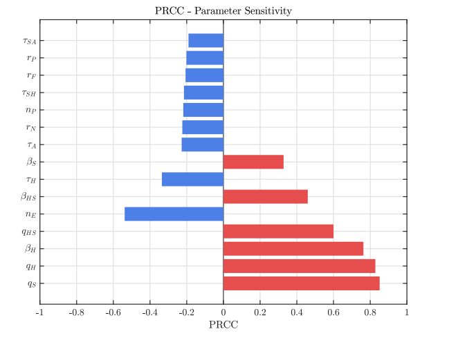
The sensitivity analysis based on PRCC revealed a clear hierarchy of influence on the total infectious burden (\(I_{N}\), \(I_{H}\), \(I_{A}\), \(I_{S}\), \(I_{HS}\), \(I_{AS}\)) within the system dynamics. The dominant determinants were the diagnosis rates, with the Syphilis diagnosis rate (\(q_S\), PRCC: \(0.851\)) and the HIV diagnosis rate (\(q_H\), PRCC: \(0.828\)) showing the highest positive coefficients. This indicates that enhanced diagnostic efficiency directly translates into a higher number of reported cases. These were followed by the HIV effective contact rate (\(\beta_H\), \(0.763\)) and the coinfection diagnosis rate (\(q_{HS}\), \(0.600\)), confirming that diagnosis and active HIV transmission are the main drivers of increases in the output metric.
In contrast, the most influential negative factor was the diagnosis rate following a risky contact (\(\eta_E\), \(-0.538\)), representing the most sensitive leverage point for infection reduction. The coinfection effective contact rate (\(\beta_{HS}\), \(0.460\)) and the HIV treatment rate (\(\tau_H\), \(-0.335\)) exhibited moderate influence. Finally, parameters with the smallest absolute effects—such as the Syphilis transmission rate (\(\beta_S\), \(0.328\)), treatment rates for advanced stages or coinfection (\(\tau_A, \tau_{SH}, \tau_{SA}\), ranging between \(-0.190\) and \(-0.228\)), and PrEP-related parameters (\(r_N, n_P, r_F, r_P\), between \(-0.202\) and \(-0.224\))—showed minor, negative contributions to prevalence reduction. These findings suggest that system sensitivity is predominantly concentrated in the detection phase and active HIV transmission, see Table 2 and Figure 2.
| Parameter | PRCC |
|---|---|
| \(q_S\) | 0.851 |
| \(q_H\) | 0.828 |
| \(\beta_H\) | 0.763 |
| \(q_{HS}\) | 0.600 |
| \(n_E\) | -0.538 |
| \(\beta_{HS}\) | 0.460 |
| \(\tau_H\) | -0.335 |
| \(\beta_S\) | 0.328 |
| \(\tau_A\) | -0.228 |
| \(r_N\) | -0.224 |
| \(n_P\) | -0.219 |
| \(\tau_{SH}\) | -0.215 |
| \(r_F\) | -0.206 |
| \(r_P\) | -0.202 |
| \(\tau_{SA}\) | -0.190 |
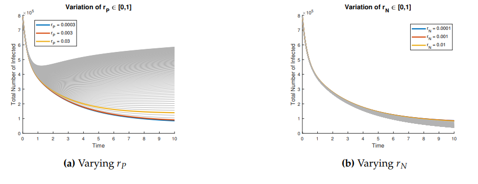
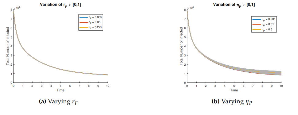
Figures 3 and 4 show the behavior of the sum of diagnosed and undiagnosed infected individuals with HIV, syphilis, and HIV–syphilis coinfection, under the independent variation of the parameters associated with PrEP (\(r_{P}, r_{N}, r_{F}, \eta_{P}\)) within their definition interval \([0,1]\).
The basic reproduction numbers for the syphilis and HIV submodels, as well as for the HIV-syphilis coinfection model, are \(\Re^{S}_{0}= 1.3336,\) \(\Re^{H}_{0}= 2.206,\) and \(\Re^{G}_{0}= 5.6379,\) respectively. These values indicate that each disease has the potential to spread within the population, as each infected individual transmits the infection, on average, to more than one susceptible person. A higher basic reproduction number corresponds to a faster rate of transmission, making the disease more challenging to control and requiring broader intervention coverage—for example, through the use of PrEP, early diagnosis, or treatment programs.
The sensitivity analysis of the basic reproduction number determines the relative importance of the parameters on the basic reproduction number. The sensitivity index can be defined using the partial derivatives, provided that the variable be differentiable with respect to the parameter under study. Sensitivity analysis also helps to identify the vitality of the parameter values in the predictions using the model [50, 57].
Definition 1. The normalized forward sensitivity index of a variable \(v\), which is differentiable with respect to a parameter \(p\), is defined as1:
\[\begin{aligned} \label{ind1} \Upsilon^{v}_{p}:=\dfrac{\partial v}{\partial p}\times \dfrac{p}{v}. \end{aligned} \tag{66}\]
We can characterize the sensitivity index as follows:
A positive value of the sensitivity index implies that an increase of the parameter value causes an increase of the basic reproduction number.
A negative value of the sensitivity index implies that an increase of the parameter value causes a decrease of the basic reproduction number.
Furthermore, a highly sensitive parameter must be estimated carefully, since a small variation in it will cause large quantitative changes [57].
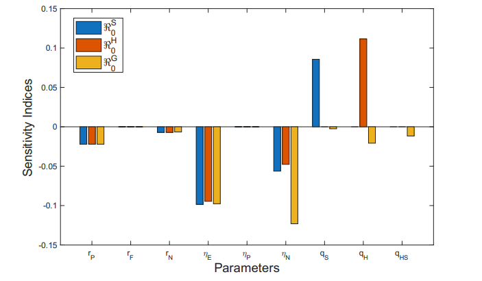
We now analyze the sensitivity indices of the basic reproduction number with respect to key parameters associated with PrEP usage. These include parameters related to PrEP use in the general population and among undiagnosed individuals or those unaware of their infection status (\(r_{P}\) and \(r_{N}\)), the rate of PrEP discontinuation or failure (\(r_{F}\)), and the diagnosis rates (\(\eta_{P}, \eta_{E}\) and \(\eta_{N}\)), those related to syphilis (\(q_{S}\)), HIV (\(q_{H}\)), and coinfection HIV and syphilis (\(q_{HS}\)).
Table 3 shows the sensitivity index values of the parameters associated with PrEP and case diagnosis in relation to the basic reproduction numbers, and also provides a brief interpretation of each result.
| Parameter | \(\Re^{S}_{0}\) | \(\Re^{H}_{0}\) | \(\Re^{G}_{0}\) |
|---|---|---|---|
| \(r_{P}\) | -0.0221 | -0.0221 | -0.0221 |
| \(r_{F}\) | -7.5825e-08 | -6.5499e-07 | -4.6816e-07 |
| \(r_{N}\) | -0.0071 | -0.0071 | -0.0066 |
| \(\eta_{E}\) | -0.0985 | -0.0946 | -0.0977 |
| \(\eta_{P}\) | 7.9677e-08 | 6.8654e-07 | 4.9071e-07 |
| \(\eta_{N}\) | -0.0563 | -0.0477 | -0.1231 |
| \(q_{S}\) | 0.0857 | – | -0.0254 |
| \(q_{H}\) | – | 0.1115 | -0.0208 |
| \(q_{HS}\) | – | – | -0.0117 |
An increase in the \(r_{P}\) leads to a moderate decrease in the three basic reproduction numbers, which may be related to the fact that, with PrEP, there are fewer exposed individuals and greater control of transmission. The influence of the parameter \(r_{F}\) is not significant (negligible), so its effect alone does not contribute to the increase or reduction of the basic reproduction numbers, and therefore does not impact the transmission of these diseases.
Parameter \(\eta_{P}\) shows small positive sensitivity indices with respect to the different basic reproduction numbers, indicating that it does not have a significant independent effect on the transmission of these diseases.”
Parameters \(q_{S}\) and \(q_{H}\) have a positive effect and are among the most influential for their respective diseases, suggesting that an increase in these parameters leads to a rise in transmission. However, when analyzing the coinfection dynamics, the opposite effect is observed (a negative impact). In this case, we are dealing with three possible dynamics and transmission routes within a single system — HIV, syphilis, and their coinfection — along with their respective treatments and diagnostic processes.
The parameters \(\eta_{E}\) and \(\eta_{N}\) exhibit negative sensitivity indices. These parameters are associated with case diagnosis following a risk exposure and diagnosis through various pathways after such exposure, differing from attempts to enroll in the PrEP program. An increase in these parameters leads to a reduction in the transmissibility of HIV, syphilis, and their coinfection, as reflected in the basic reproduction number. This underscores that strengthening case detection after risk exposures and increasing testing rates for these diseases have a positive impact on the community. However, achieving this requires efforts to raise awareness and disseminate information about the consequences of risky contacts and the importance of early diagnosis.
Figure 5 graphically displays the sensitivity indices of each parameter with respect to the basic reproduction numbers.
Through sensitivity indices, we analyze how each parameter independently may influence the basic reproduction number, and thus the transmissibility of HIV, syphilis, and their coinfection. However, an important question arises: can the combined influence of two or more parameters have a greater positive impact on reducing the basic reproduction numbers in this scenario?
Now, we will study the joint variation of the parameters associated with the use of PrEP in the community, the diagnosis of cases through the PrEP program, and the failure or desistence rate in the use of PrEP.
First, we examine the joint variation of \(r_p\) and \(r_f\), as the combination of these parameters determines entry into the PrEP program and exit due to various causes. Figures 6–8 show the variation of these parameters on the basic reproduction numbers. For the different basic reproduction numbers associated with the dynamics of syphilis, HIV, and HIV–syphilis coinfection, we observe analogous behavior: when \(r_p\) decreases, the basic reproduction numbers exceed one. However, when \(r_p\) increases, the basic reproduction numbers decrease significantly, reaching values well below one, which is a positive effect.
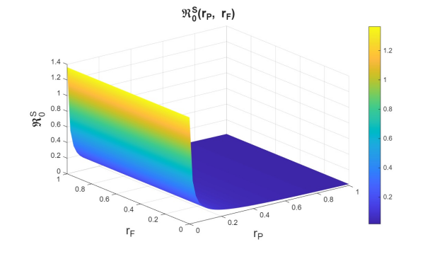
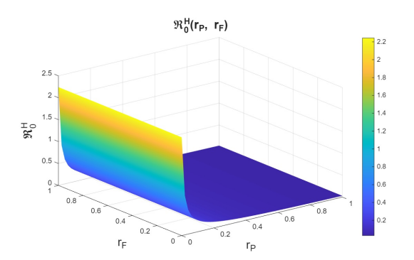
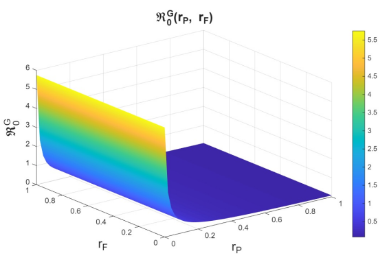
We can conclude that \(r_p\) has a strong influence on the dynamics because, despite an increase in the dropout or failure rate in PrEP use, its growth helps prevent the increase in basic reproduction numbers—i.e., it reduces disease transmissibility.
In the joint variation of \(r_p\) and \(n_p\), which represents the relationship between the use of PrEP in the community and the diagnosis of cases associated with the attempt to enter the PrEP program, we observed behavior analogous to the variation of \(r_p\) and \(r_f\) (see Figures 9–11). We find that, if we increase \(r_p\), regardless of the behavior of \(n_p\), the basic reproduction numbers decrease significantly, reaching values below one. However, when \(r_p\) decreases, the basic reproduction numbers can exceed one, which increases the transmissibility of syphilis, HIV, and HIV–syphilis coinfection. These results highlight the influence of PrEP use in the population with respect to the diagnosis of cases linked to attempts to enter the PrEP program.
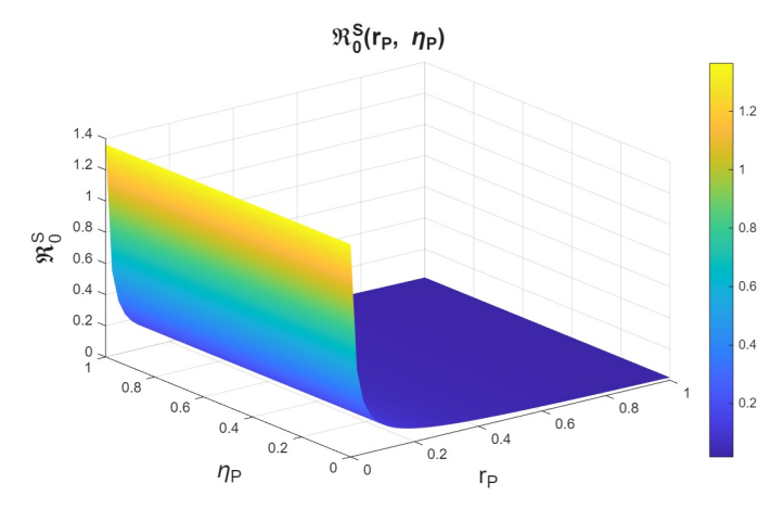
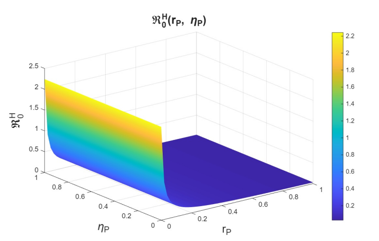
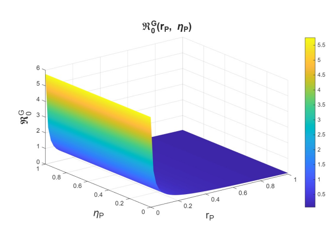
We can conclude that \(r_p\), the rate of PrEP use among the susceptible population, has a strong influence on the dynamics in relation to both the dropout or failure rate in PrEP use and the diagnosis of cases associated with attempts to enter the PrEP program. Increasing PrEP use in the susceptible population has a significant effect in the studied scenario, as, according to the behavior and interpretation of the basic reproduction numbers, it reduces the transmissibility of syphilis, HIV, and HIV–syphilis coinfection.
Now, we study \(r_n\), which is the rate at which infected individuals who are undiagnosed or unaware of their status attempt to enter the PrEP program, in combination with \(\eta_p\). Here, we observe behavior analogous to that seen in the study of variation with \(r_p\) (see Figures 12–14). The behavior observed in the variation of \(r_n\) with \(\eta_{P}\) is analogous to that of the variation of \(r_p\) with \(\eta_{P}\) (see Figures 15-17). Therefore, we can conclude that \(r_n\) also has a strong influence on the dynamics.
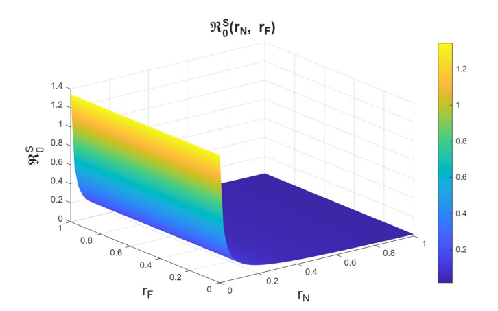
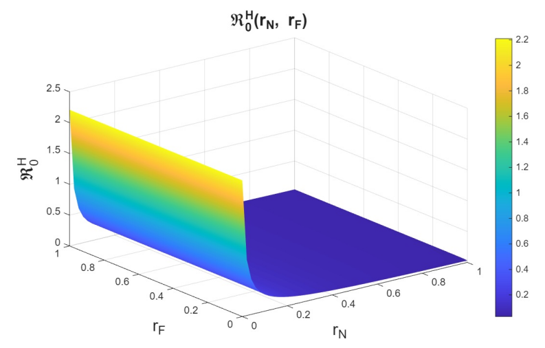
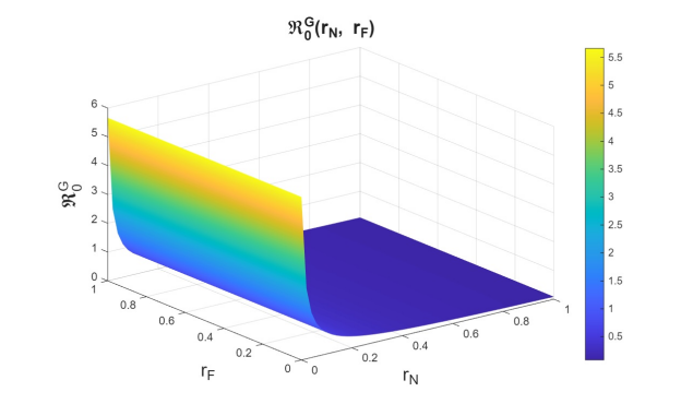
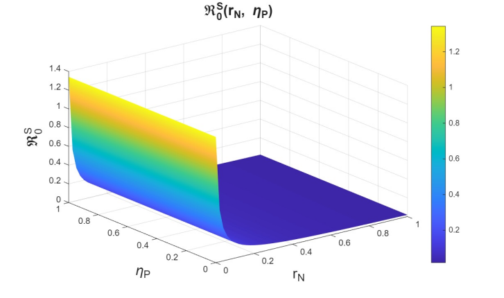
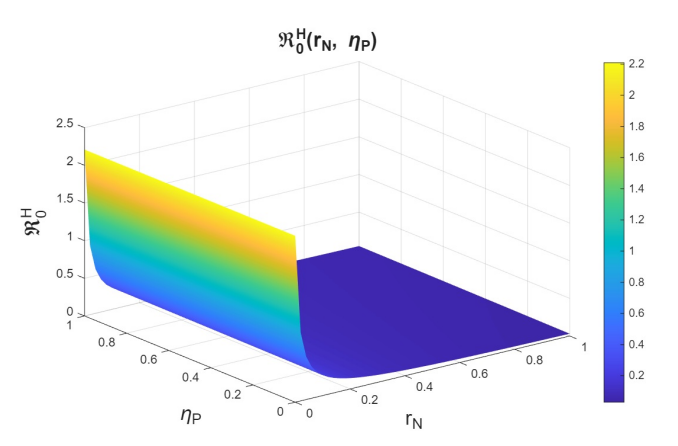
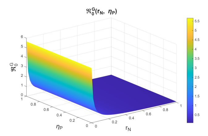
Through the study of the basic reproduction numbers in the considered scenario—focusing on the implementation of the PrEP program and its impact on case diagnosis—we were able to confirm that the PrEP program has a positive effect in reducing transmission not only of HIV, but also of syphilis and HIV–syphilis coinfection. The parameters associated with PrEP use in the community and with the diagnosis of infected individuals attempting to enter the PrEP program—specifically those infected who are unaware of their status—have a strong influence on the dynamics. Their increase produces a positive effect, significantly reducing the basic reproduction numbers; that is, the transmissibility of these diseases within the community.
The information obtained in this study shows that the dissemination and expansion of the PrEP program can be a powerful tool in the fight not only against HIV, but also against syphilis and HIV–syphilis coinfection.
The objective of this section is to quantify the impact of the PrEP program on the diagnosis of new cases of HIV, syphilis, and HIV-syphilis coinfection. While maintaining the current conditions for syphilis treatment and antiretroviral therapy, we also assess how many cases are reported as recovered from syphilis and how many individuals achieve adherence to HIV treatment, leading to improved immune status and, most importantly, an undetectable viral load in the blood.
To this end, we will construct two scenarios by increasing PrEP uptake rates among susceptible individuals and among infected individuals who are either undiagnosed or unaware of their infection status, while simultaneously decreasing the rate of PrEP discontinuation or failure:
Scenario I: \(r_{P}=0.003\), \(r_{N}=0.001\), and \(r_{F}=0.05\).
Scenario II: \(r_{P}=0.03\), \(r_{N}=0.01\), and \(r_{F}=0.005\).
The scenarios were constructed by increasing the PrEP uptake rate and decreasing the rate of PrEP discontinuation or failure.
We can conclude that increasing PrEP use in the population and reducing the rate of PrEP discontinuation or failure leads to a greater number of diagnosed cases of syphilis, HIV, and HIV-syphilis coinfection. This is a positive outcome, as these individuals are indeed infected and part of the transmission dynamics, meaning they can spread the diseases if undiagnosed (see Figures 18-20). Diagnosis plays a crucial role, as it enables appropriate treatment: syphilis can be cured, and in the case of HIV, antiretroviral therapy prevents progression to AIDS and leads to undetectable viral loads in the blood, thereby preventing further transmission.
With increased PrEP use in the general population—closely linked to the availability of treatment and awareness campaigns—and a reduction in discontinuation or treatment failure, efforts can focus on encouraging individuals to remain adherent. This includes the potential incorporation of strategies to improve adherence, such as long-acting injectable PrEP (pre-exposure prophylaxis), which has emerged in recent years as a highly effective alternative to daily oral pills for HIV prevention [51].
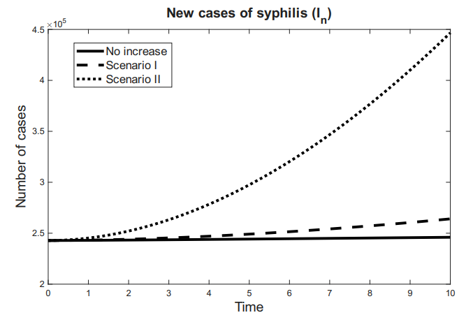
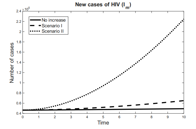
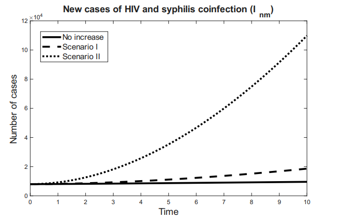
We now focus on analyzing the number of individuals recovered from syphilis and those successfully treated for HIV. To assess the isolated impact of PrEP, we maintain constant treatment rates for both syphilis and HIV across all scenarios.
Both the number of recovered syphilis cases and the number of treated HIV-positive individuals, as well as their combination, increase as PrEP use rises in the general population (including susceptibles and undiagnosed infected individuals), as shown in Figures 21-23. Although new cases also increase, the number of treated and recovered individuals grows accordingly. This indicates that the inclusion of individuals in the PrEP program has a positive effect by increasing the proportion of cases that no longer negatively impact the transmission dynamics.
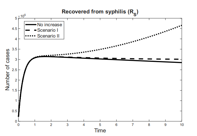
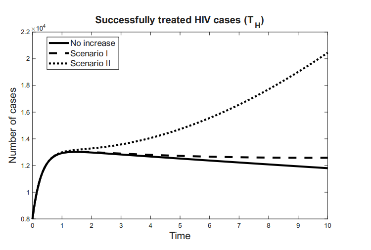
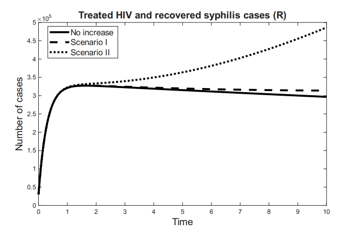
We can conclude that the increase in PrEP use and the reduction in discontinuation and failure rates have a positive effect on mitigating the impact of syphilis, HIV, and HIV-syphilis coinfection within the community. Assuming the availability of effective treatments for both syphilis and HIV, the PrEP program facilitates the diagnosis of new cases and their subsequent treatment, which can lead to syphilis recovery or prevent HIV progression, improve patients’ quality of life, and, by achieving an undetectable viral load, prevent further virus transmission.
This study developed a mathematical model to evaluate the impact of pre-exposure prophylaxis (PrEP) on the transmission and diagnosis of HIV, syphilis, and their coinfection. The findings underscore PrEP’s potential not only as a preventive tool against HIV but also as an indirect mechanism for enhancing the detection and control of other sexually transmitted infections. The model incorporates coinfection during high-risk sexual encounters, differential treatment outcomes, and diagnostic pathways, both standard and those initiated through PrEP enrollment. Notably, it captures the continued vulnerability of PrEP users to syphilis infection despite their protection from HIV.
We first analyzed submodels for HIV and syphilis independently, establishing host population persistence and calculating basic reproduction numbers in the absence of PrEP. This foundational analysis underscored the need for intervention strategies. After integrating PrEP into the full model, we derived theoretical conditions under which variations in PrEP-associated parameters—especially those influencing diagnosis—do not adversely affect transmission dynamics.
A sensitivity analysis confirmed that increasing PrEP uptake among susceptible individuals consistently reduces the basic reproduction numbers for HIV, syphilis, and coinfection. For parameters whose effects depend on contextual interactions, we identified conditions ensuring a positive public health impact. These results highlight PrEP’s potential as both a preventive and diagnostic tool.
Computational simulations validated the theoretical findings and assessed the effect of changes in PrEP-related parameters. Scenarios involving increased PrEP uptake and reduced discontinuation rates showed consistent reductions in the reproduction numbers and transmissibility of all three epidemics.
Furthermore, expanded PrEP use led to increased diagnosis and treatment of infections, particularly benefiting syphilis cure rates and HIV viral suppression. These findings reinforce the dual preventive and therapeutic impact of PrEP, especially when delivered through adherence-enhancing strategies such as long-acting injectable formulations.
In future research, we plan to calibrate the proposed model using real epidemiological data to better reproduce observed dynamics. Furthermore, we aim to extend this framework to investigate the broader impact of PrEP on other HIV-associated infections and comorbidities, strengthening its relevance for public health decision-making.
The authors declare they have not used Artificial Intelligence (AI) tools in the creation of this article.