
The Sitnikov problem describes the motion of a particle of negligible mass attracted by two equal masses \(m_{1} =m_{2} =\frac{1}{2}\). The primaries \(m_{1}\) and \(m_{2}\) move on the plane \((x,y)\), following an elliptic motion with eccentricity \(e\in [0,1)\), while the massless body \(m_{3}\) performs motion along an axis perpendicular to the primary orbit plane through the barycentre of the primaries. The minimal period of the elliptic motion is \(2\pi\) if the gravitational constant is assumed to be \(G=1\). If \(z\) denotes the position of the particle \(m_{3}\) in a coordinate system with origin at the centre of mass of the primaries, then the equation of motion of the Sitnikov problem becomes
\[\label{GrindEQ__1_1_} \ddot{z}+\frac{z}{(z^{2} +r(t,e)^{2} )^{3/2} } =0\mathrm{} , \tag{1}\] where \(z\) is the distance from the centre of the orbit to \(m_{3}\), \(\ddot{z}\) is acceleration, \(e\) is eccentricity and \(r(t,e)\) is the distance of the primaries to their center of mass and it is given by \[\label{GrindEQ__1_2_} r(t,e)=\frac{1-e\cos \; u(t)}{2} , \tag{2}\]
\[\label{GrindEQ__1_3_} \ddot{r}=\frac{1-e^{2} }{16r^{3} } -\frac{1}{8r^{2} } , \tag{3}\] with eccentricity \(e=0\) or \(0<e<1\), respectively. Here \(u(t)\) is the eccentricity anomaly which is a function of time through Kepler equation
\[\label{GrindEQ__1_4_} u-e\sin u(t)=t\mathrm{} , \tag{4}\] without loss of generality, when \(0<e<1\), we take the origin of time in such a way that at \(t=0\) the primaries are at the pericenter of the ellipse. We note that system (1) depends on one parameter, the eccentricity \(e\in [0,1)\) when the eccentricity \(e\) is zero (that is, the primaries move on the circular orbit \(r(t)=\frac{1}{2}\) of the Kepler problem (3), (1) becomes the equation of motion \(\ddot{z}=-\frac{z}{(z^{2} +\frac{1}{4} )^{3/2} }\) for the circular Sitnikov problem.
More information can be found in [1] and in the more recent [2]. The existence of symmetric (even or odd) periodic solutions has been discussed in [3– 6]. In [3], methods of local analysis were employed, and they got results which are valid only for small eccentricity e. The papers [4, 5] considered arbitrary eccentricity from a theoretical perspective by using the global continuation method due to Leray and Schauder, and [5] found families of symmetric periodic solutions bifurcating from the equilibrium at the center of mass. These families were labelled according to the number of zeros in the same fashion as it occurs in the work by [7] for other non-linearities [6] combines Shooting arguments with Sturm comparison theory to prove the existence of odd periodic solutions with a prescribed number of zeros.
While [8] presents a very complete description of the set of symmetric periodic solutions based on numerical computations, [9] discussed on the circular Sitnikov problem as a subsystem of the three-dimensional circular restricted three-body problem, where they used elliptic functions to give the analytical expressions for the solutions of the circular Sitnikov problem and for the period function of its family of periodic orbits. They also analyzed the qualitative and quantitative behaviour of the period function. The purpose of this study is to obtain numerical results for all values of the eccentricity using only very elementary tool, the fourth-order Runge-Kutta method. This paper is divided into sections: §1 is the introduction of the Sitnikov problem, §2 is the definition and theorems which was used in the result while §3 is the derivation of the fourth-order Runge-Kutta method, and §4 is the result obtained with numerical simulations with conclusion.
Definition 1 (Precision of the Runge-Kutta method). .
Assume that \(y(t)\) is the solution of the problem \[\label{GrindEQ__2_1_} y^{n} =f'\left(t,y\right) . \tag{5}\]
If \(y\left(t\right)\in C^{3} ,\left[t_{0} ,b\right]\) and \(\left(t_{i} ,y_{i} \right)^{m} =0\) is the sequence of approximations generated by the Runge-Kutta method of order 2, then \[\label{GrindEQ__2_2_} \left|E_{i} \right|=\left|y\left(t_{i} \right)-y_{i} \right|=0\left(h^{2} \right), \tag{6}\] \[\label{GrindEQ__2_3_} \left|E_{i+1} \right|=\left|y\left(t_{i+1} \right)-y_{i} -hTN\left(t,y_{i} \right)\right|=0\left(h^{3} \right). \tag{7}\]
Given the interval \(\left[t_{0} ,b\right]\), we satisfy that \[\label{GrindEQ__2_4_} E\left(y^{\left(b\right)} ,h\right)=\left[y^{\left(b\right)} ,y^{m} \right]=0\left(h^{2} \right) . \tag{8}\]
Definition 2. Assume the existence of such a solution \(y\left(t\right)\) is guaranteed and unique, provided\(f\left(t,y\right)\),
i. is continuous in the infinite strip \[\label{GrindEQ__2_5_} E=\left\{x_{0} \le x\le T,\left|y\right|<\infty \right\} . \tag{9}\]
ii. is more specifically Lipchitz continuous in the dependent variable \(y\) over the same region \(R\), that is there exist a positive constant \(L\) such that for all \(\left(t,y\right),\left(t,y'\right)\in R\) \[\left|f\left(t,y\right)-f\left(t,y'\right)\right|<L\left|y-y'\right|.\]
Theorem 1. Suppose that \(\sigma\) is a nonempty, closed and bounded limit set of a planar flow, then one of the following holds:
i. \(\sigma\) is an equilibrium point,
ii. \(\sigma\) is a periodic solution,
iii. \(\sigma\) consists of a set of equilibria and connecting orbits between these equilibria.
Proof. We consider \(\sigma =w\left(x\right)\) for some \(x\in {\mathbb R}^{2}\). The argument in the case of a \(\sigma -\) limit set is similar. Let \(y\in w\left(x\right)\) and \(z\in w\left(y\right)\). If \(z\) is not an equilibrium point, then \(w\left(y\right)\) must be a periodic solution and if \(w\left(y\right)\) is a periodic solution then \(w\left(x\right)=w\left(y\right)\) and thus \(w\left(x\right)\) is also a periodic solution. Now we assume that \(z\in w\left(y\right)\) is equilibrium point. Then \(w\left(y\right)\) must consist entirely of equilibria since if there is a point \(z\in w\left(y\right)\) that is not equilibrium, then we know that \(w\left(y\right)\) is a periodic solution (and in particular contains no equilibrium). We note that since \(y\in w\left(x\right)\) it follows that\(\left\{\phi ^{t} \left(y\right)\right\}_{t\in {\mathbb R}} \subset w\left(x\right)\), where \(\phi ^{t}\) denotes the time \(\left(t\right)\) flow.
Hence, \(\alpha \left(y\right)\in w\left(x\right)\) and for the same reasons as before, \(\alpha \left(y\right)\) must be equilibrium otherwise \(w\left(y\right)\) and \(w\left(x\right)\) must be a periodic solution. Hence, we find that either \(y\) is an equilibrium point, or \(y\) lies in the intersection between the stable and unstable manifolds of the equilibria \(w\left(y\right)\) and\(\alpha \left(y\right)\). Theorem\(\mathrm{\}}\) for each integer\(m\ge 1\), there exists a unique solution \(z\left(t\right)\) of (1) satisfying the conditions \[\label{GrindEQ__2_6_} z\left(t+2mt\right)=z\left(t\right),\qquad z\left(-t\right)=-z\left(t\right),\qquad t\in {\mathbb R} , \tag{10}\] \[\label{GrindEQ__2_7_} z\left(t\right)>0,\qquad t\in \left[0,m\pi \right]\mathrm{} . \tag{11}\]
The variational equation at the centre of mass \(z=0\) will play an important role, it is the equation of Hill’s type, [10]; \[\label{GrindEQ__2_8_} \ddot{\xi }+\frac{1}{r\left(t,e\right)^{3} } \xi =0\mathrm{} . \tag{12}\] ◻
Theorem 2. Assume that \(m\ge 1\) and \(N\ge 0\) are given integers, then the following statements are equivalent.
(a) There exist a solution of (1) satisfying the condition in (10) and having exactly \(N\) zero in the interval \(\left[0,m\pi \right]\);
(b) The solution \(\xi \left(t\right)\) of (12) with initial conditions \(\xi \left(0\right)=0,\xi \left(0\right)=1\) has more than \(N\) zero in \(\left[0,m\pi \right]\).
The simple Euler method comes from using just one term from the Taylor series for \(y(x)\) expanded about \(x=x_{0}\).
The modified Euler method can also be derived from using terms \[\label{GrindEQ__2_9_} y(x_{0} +h)=y(x_{0} )+y'(x_{0} )\cdot h+y''(x_{0} )\frac{h^{2} }{2}. \tag{13}\]
If we replace the second derivative with a backward-difference approximation, \[\label{GrindEQ__3_0_} y(x_{0} +h)=y(x_{0} )+y'(x_{0} )\cdot h+\left[\frac{y'(x_{0} +h)-y'(x_{0} )}{h} \right]\frac{h^{2} }{2} =y(x_{0} )+\frac{y'(x_{0} )+y'(x_{0} +h)}{2} h , \tag{14}\] we get the formula for the modified method. What if we use more terms of the Taylor series?
Two German mathematicians, Runge and Kutta, developed algorithms from using more than two terms of the series. We will consider only fourth-order formula. The modified Euler method is a second-order Runge-Kutta method. The Second-order Runge-Kutta methods are obtained by using a weighted average of two increments to \(y(x_{0} ),k_{1}\) and \(k_{2}\). For the equation \(\frac{dy}{dx} =f(x,y)\); \[\label{GrindEQ__3_1_} \left\{\begin{array}{l} {y_{n+1} =y_{n} +ak_{1} +bk_{2} ,} \\ {k_{1} =hf(x_{n} ,y_{n} ),} \\ {k_{2} =hf(x_{n} +ah,y_{n} +\beta k_{1} ).\quad } \end{array} \right. \tag{15}\]
We can think of the values \(k_{1}\) and \(k_{2}\) as estimates of the change in \(y\) when \(x\) advances by \(h\), because they are the product of the change in \(x\) and a value for the slope of the curve, \(\frac{dy}{dx}\).
The Runge-Kutta methods always use the simple Euler estimate as the first of \(\Delta y\); the other estimate is taken with \(x\) and \(y\) stepped up by the fractions \(\alpha\) and \(\beta\) of \(h\) and of the earlier estimate of \(\Delta y,k_{1}\). Our interest is to devise a scheme of choosing the four parameters \(a,b,\alpha ,\beta\). We make Eq. (15) agree as well as possible with the Taylor-series expansion, in which the \(y-\) derivatives are written in terms off, from \(\frac{dy}{dx} =f(x,y),\) \[y_{n+1} =y_{n} +hf(x_{n} ,y_{n} )+\frac{h^{2} }{2} f'(x_{n} ,y_{n} )+….\]
An equivalent form, because \(\frac{df}{dx} =f_{x} +f_{y}\), \(\frac{dy}{dx} =f_{x} +f_{y}\), is \[\label{GrindEQ__3_2_} y_{n+1} =y_{n} +hf_{n} +h^{2} \left(\frac{1}{2} f_{x} +\frac{1}{2} f_{y} \right)f_{n} \mathrm{} . \tag{16}\] [All the derivatives in Eq. (16) are calculated at the point\((x_{n} ,y_{n} )\).] We now rewrite Eq. (16) by substituting the definitions of \(k_{1}\) and \(k_{2}\).
\[\label{GrindEQ__3_3_} y_{n+1} =y_{n} +ahf(x_{n} ,y_{n} )+bhf[x_{n} +ah,y_{n} +\beta hf(x_{n} ,y_{n} )] . \tag{17}\]
To make the last term of Eq. (17) comparable to Eq. (16), we expand \(f(x,y)\) in a Taylor series in terms of \(x_{n} ,y_{n}\) remembering that \(f\) is a function of two variables, retaining only first derivative terms: \[\label{GrindEQ__3_4_} f[x_{n} +ah,y_{n} +\beta hf(x_{n} ,y_{n} )]=(f+f_{x} ah+f_{y} \beta hf_{n} ) . \tag{18}\]
On the right side of both Eqs. (16) and (18), \(f\) and its partial derivatives are all to be evaluated at \((x_{n} ,y_{n} )\).
Substituting from Eq. (18) into Eq. (17), we have \[\label{GrindEQ__3_5_} y_{n+1} =y_{n} +(a+b)hf_{n} +h^{2} (abf_{x} +\beta bf_{y} )f_{n} . \tag{19}\]
Eq. (19) will be identical to Eq. (16) if \(a+b=1,\;ab=\frac{1}{2} ,\;\beta b=\frac{1}{2}\).
Note that only three equations need to be satisfied by the four unknowns. We can choose one value arbitrary (with minor restrictions); hence, we have a set of second-order methods.
One choice can be \(a=0,\;b=1;\;\alpha =\beta =\frac{1}{2}\). this gives the midpoint method.
Another choice can be \(a=\frac{1}{2} ,\;b=\frac{1}{2} ;\;\alpha =1,\;\beta =1\), which gives the modified Euler.
Still another possibility is \(a=\frac{1}{3} ,\;b=\frac{2}{3} ;\;\alpha =\frac{3}{4} ,\;\beta =\frac{3}{4}\); this is said to give a minimum bound to the error. All of these are special cases of second-order of Runge-Kutta methods.
Fourth-order Runge-Kutta methods are most widely used and are derived in similar fashion.
Greater complexity results from having to compare terms through \(h^{4}\) , and this gives a set of 11 equations in 13 unknowns. The set of 11 equations can be solved with 2 unknowns being chosen arbitrarily. It needs four values of function in each step iteration. The most commonly used set of values leads to the procedure; \[\label{GrindEQ__3_6_} \left\{\begin{aligned} y_{n+1} &= y_n + \frac{1}{6}(k_1 + 2k_2 + 2k_3 + k_4), \\ k_1 &= h f(x_n, y_n) ,\\ k_2 &= h f\left(x_n + \frac{1}{2}h, y_n + \frac{1}{2}k_1\right) ,\\ k_3 &= h f\left(x_n + \frac{1}{2}h, y_n + \frac{1}{2}k_2\right), \\ k_4 &= h f(x_n + h, y_n + k_3). \end{aligned}\right. \tag{20}\]
This Runge-Kutta method will be used to solve Eq. (1) in §4 numerically.
Considering Eq. (1); let \(\dot{z}=\varphi\), such that \(\ddot{z}=\dot{\varphi }\) therefore, Eq. (1) becomes \[\label{GrindEQ__3_7_} \dot{\varphi }=-\frac{z}{\left(z^{2} +r\left(t,e\right)^{2} \right)^{{}^{3} /_{2} } } . \tag{21}\]
But from Theorem 2, Eq. (17) states \[\label{GrindEQ__3_8_} \dot{\varphi }=-\frac{1}{r\left(t,e\right)^{3} } y\text{ at }\xi =y . \tag{22}\]
Which is linear (Hill’s type of equation at\(z=0\)).
Fourth-Order Runge –Kutta methods \[\label{GrindEQ__3_9_} y_{n+1} =y_{n} +\frac{1}{6} \left(k_{1} +2k_{2} +2k_{3} +k_{4} \right) . \tag{23}\]
Given \(r\left(t,e\right)=\frac{1}{2} \left(1-e\cos u\left(t\right)\right)\), let \(u\left(t\right)=0\), \(e\in \left[0,1\right]\),\(h=0.02\), \(y\left(0\right)=0\), \(f_{0} =1\). Approximate solutions for fourth-Order RK method with 0 \(\mathrm{\le}\) e \(\mathrm{\le}\) 1 is given in Table 1
| \(e\)(eccentricity) | \(y_{n}\)(solutions) | \(k_{1}\)(1\({}^{st}\) function) | \(k_{2}\)(2\({}^{nd}\) function) | \(k_{3}\)(3\({}^{rd}\) function) | \(k_{4}\)(4\({}^{th}\) function) |
|---|---|---|---|---|---|
| 0 | 0 | 0 | 0 | 0 | 0 |
| 0.02 | 0.002825 | 0.02 | \(-\)0.001649 | \(1.4\times 10^{-4}\) | \(-2.3\times 10^{-5}\) |
| 0.04 | 0.002371 | \(-4.8\times 10^{-4}\) | \(-4.5\times 10^{-4}\) | \(-4.6\times 10^{-4}\) | \(-4.3\times 10^{-4} \;\) |
| 0.06 | 0.001920 | \(-4.3\times 10^{-4} \;\) | \(-4.0\times 10^{-4} \;\) | \(-4.1\times 10^{-4} \;\) | \(-6.6\times 10^{-4} \;\) |
| 0.08 | 0.001573 | \(-3.7\times 10^{-4} \;\) | \(-3.5\times 10^{-4} \;\) | \(-3.5\times 10^{-4} \;\) | \(-3.2\times 10^{-4} \;\) |
| 0.10 | 0.001272 | \(-3.2\times 10^{-4} \;\) | \(-3.0\times 10^{-4} \;\) | \(-3.0\times 10^{-4} \;\) | \(-2.8\times 10^{-4} \;\) |
| 0.12 | 0.001014 | \(-2.8\times 10^{-4} \;\) | \(-2.6\times 10^{-4} \;\) | \(-2.6\times 10^{-4} \;\) | \(-2.4\times 10^{-4} \;\) |
| 0.14 | \(7.95\times 10^{-4} \;\) | \(-2.4\times 10^{-4} \;\) | \(-2.2\times 10^{-4} \;\) | \(-2.2\times 10^{-4} \;\) | \(-2.0\times 10^{-4} \;\) |
| 0.16 | \(6.13\times 10^{-4} \;\) | \(-2.0\times 10^{-4} \;\) | \(-1.8\times 10^{-4} \;\) | \(-1.8\times 10^{-4} \;\) | \(-1.7\times 10^{-4} \;\) |
| 0.18 | \(4.64\times 10^{-4} \;\) | \(-1.7\times 10^{-4} \;\) | \(-1.5\times 10^{-4} \;\) | \(-1.5\times 10^{-4} \;\) | \(-1.4\times 10^{-4} \;\) |
| 0.20 | \(3.43\times 10^{-4} \;\) | \(-1.4\times 10^{-4} \;\) | \(-1.2\times 10^{-4} \;\) | \(-1.2\times 10^{-4} \;\) | \(-1.1\times 10^{-4} \;\) |
| 0.22 | \(2.50\times 10^{-4} \;\) | \(-1.1\times 10^{-4} \;\) | \(-9.0\times 10^{-5} \;\) | \(-9.3\times 10^{-5} \;\) | \(-8.4\times 10^{-5} \;\) |
| 0.24 | \(1.76\times 10^{-4} \;\) | \(-8.4\times 10^{-5} \;\) | \(-7.3\times 10^{-5} \;\) | \(-7.5\times 10^{-5} \;\) | \(-6.4\times 10^{-5} \;\) |
| 0.26 | \(1.20\times 10^{-4} \;\) | \(-6.4\times 10^{-5} \;\) | \(-5.5\times 10^{-5} \;\) | \(-5.6\times 10^{-5} \;\) | \(-4.7\times 10^{-5} \;\) |
| 0.28 | \(7.96\times 10^{-5} \;\) | \(-4.7\times 10^{-5} \;\) | \(-4.0\times 10^{-5} \;\) | \(-4.1\times 10^{-5} \;\) | \(-3.4\times 10^{-5} \;\) |
| 0.30 | \(5.09\times 10^{-5} \;\) | \(-3.4\times 10^{-5} \;\) | \(-2.8\times 10^{-5} \;\) | \(-2.9\times 10^{-5} \;\) | \(-2.4\times 10^{-5} \;\) |
| 0.32 | \(3.13\times 10^{-5} \;\) | \(-2.4\times 10^{-5} \;\) | \(-1.9\times 10^{-5} \;\) | \(-2.0\times 10^{-5} \;\) | \(-1.6\times 10^{-5} \;\) |
| 0.34 | \(1.84\times 10^{-5} \;\) | \(-1.6\times 10^{-5} \;\) | \(-1.2\times 10^{-5} \;\) | \(-1.3\times 10^{-5} \;\) | \(-9.9\times 10^{-6} \;\) |
| 0.36 | \(1.03\times 10^{-5} \;\) | \(-1.0\times 10^{-5} \;\) | \(-7.8\times 10^{-6} \;\) | \(-8.5\times 10^{-6} \;\) | \(-6.1\times 10^{-6} \;\) |
| 0.38 | \(5.44\times 10^{-6} \;\) | \(-6.3\times 10^{-6} \;\) | \(-4.6\times 10^{-6} \;\) | \(-5.1\times 10^{-6} \;\) | \(-3.5\times 10^{-6} \;\) |
| 0.40 | \(2.70\times 10^{-6} \;\) | \(-3.7\times 10^{-6} \;\) | \(-2.5\times 10^{-6} \;\) | \(-2.9\times 10^{-6} \;\) | \(-1.9\times 10^{-6} \;\) |
| 0.42 | \(1.24\times 10^{-6} \;\) | \(-2.0\times 10^{-6} \;\) | \(-1.3\times 10^{-6} \;\) | \(-1.6\times 10^{-6} \;\) | \(-9.1\times 10^{-7} \;\) |
| 0.44 | \(5.26\times 10^{-7} \;\) | \(-1.0\times 10^{-6} \;\) | \(-6.3\times 10^{-7} \;\) | \(-7.9\times 10^{-7} \;\) | \(-4.0\times 10^{-7} \;\) |
| 0.46 | \(2.04\times 10^{-7} \;\) | \(-4.8\times 10^{-7} \;\) | \(-2.8\times 10^{-7} \;\) | \(-3.7\times 10^{-7} \;\) | \(-1.6\times 10^{-7} \;\) |
| 0.48 | \(7.20\times 10^{-8} \;\) | \(-2.1\times 10^{-7} \;\) | \(-1.1\times 10^{-7} \;\) | \(-1.6\times 10^{-7} \;\) | \(-4.9\times 10^{-8} \;\) |
| 0.50 | \(2.28\times 10^{-8} \;\) | \(-8.2\times 10^{-8} \;\) | \(-3.7\times 10^{-8} \;\) | \(-6.4\times 10^{-8} \;\) | \(-9.9\times 10^{-9} \;\) |
| 0.52 | \(1.36\times 10^{-8} \;\) | \(-2.9\times 10^{-8} \;\) | \(-1.1\times 10^{-8} \;\) | \(-2.3\times 10^{-8} \;\) | \(4.3\times 10^{-8} \;\) |
| 0.54 | \(3.68\times 10^{-9} \;\) | \(-1.9\times 10^{-8} \;\) | \(-5.8\times 10^{-9} \;\) | \(-1.7\times 10^{-8} \;\) | \(4.8\times 10^{-9} \;\) |
| 0.56 | \(1.03\times 10^{-9} \;\) | \(-6.1\times 10^{-9} \;\) | \(-1.2\times 10^{-9} \;\) | \(-5.4\times 10^{-9} \;\) | \(3.3\times 10^{-9} \;\) |
| 0.58 | \(3.46\times 10^{-10} \;\) | \(-1.9\times 10^{-9} \;\) | \(-1.3\times 10^{-10} \;\) | \(-1.9\times 10^{-9} \;\) | \(1.9\times 10^{-9} \;\) |
| 0.60 | \(1.72\times 10^{-10} \;\) | \(-7.5\times 10^{-10} \;\) | \(6.4\times 10^{-11} \;\) | \(-8.8\times 10^{-10} \;\) | \(1.3\times 10^{-9} \;\) |
| 0.62 | \(1.78\times 10^{-10} \;\) | \(-4.3\times 10^{-10} \;\) | \(1.4\times 10^{-10} \;\) | \(-7.6\times 10^{-10} \;\) | \(1.7\times 10^{-9} \;\) |
| 0.64 | \(3.08\times 10^{-10} \;\) | \(-5.2\times 10^{-10} \;\) | \(2.6\times 10^{-10} \;\) | \(-9.7\times 10^{-10} \;\) | \(2.7\times 10^{-9} \;\) |
| 0.66 | \(1.13\times 10^{-9} \;\) | \(-1.1\times 10^{-9} \;\) | \(8.3\times 10^{-10} \;\) | \(-2.7\times 10^{-9} \;\) | \(9.7\times 10^{-9} \;\) |
| 0.68 | \(9.15\times 10^{-9} \;\) | \(-4.6\times 10^{-9} \;\) | \(5.2\times 10^{-9} \;\) | \(-1.7\times 10^{-8} \;\) | \(7.6\times 10^{-8} \;\) |
| 0.70 | \(1.74\times 10^{-7} \;\). | \(-4.5\times 10^{-8} \;\) | \(7.1\times 10^{-8} \;\) | \(-2.4\times 10^{-7} \;\) | \(1.4\times 10^{-6} \;\) |
| 0.72 | \(8.05\times 10^{-6} \;\) | \(-1.0\times 10^{-6} \;\) | \(2.2\times 10^{-6} \;\) | \(-8.5\times 10^{-6} \;\) | \(6.1\times 10^{-5} \;\) |
| 0.74 | \(9.54\times 10^{-4} \;\) | \(-5.9\times 10^{-5} \;\) | \(1.7\times 10^{-4} \;\) | \(-7.7\times 10^{-4} \;\) | \(6.9\times 10^{-3} \;\) |
| 0.76 | 0.763069 | \(-8.7\times 10^{-3} \;\). | 0.034769 | \(-0.188087\) | 1.077431 |
| 0.78 | 721.703614 | \(-8.831817\;\) | 48.063684 | \(-326.248829\) | 4890.845379 |
| 0.80 | 2165610.343 | \(-10844.53214\) | 81210.45169 | \(-714010.5297\) | 14265776.52 |
| 0.82 | \(2.28\times 10^{10}\) | \(-43312206.86\;\) | 454655036.4 | \(-5353389789\) | \(1.5\times 10^{11}\) |
| 0.84 | \(9.61\times 10^{14}\) | \(-6.26\times 10^{11} \;\) | \(9.45\times 10^{12} \;\) | \(-1.55\times 10^{14}\) | \(6.1\times 10^{15}\) |
| 0.86 | \(1.95\times 10^{20}\) | \(-3.8\times 10^{16} \;\) | \(8.4\times 10^{17} \;\) | \(-2.0\times 10^{19}\) | \(1.2\times 10^{21}\) |
| 0.88 | \(2.19\times 10^{26}\) | \(-1.1\times 10^{22} \;\) | \(4.0\times 10^{23} \;\) | \(-1.5\times 10^{25}\) | \(1.3\times 10^{27}\). |
| 0.90 | \(1.90\times 10^{33}\) | \(-2.0\times 10^{28} \;\) | \(1.2\times 10^{30} \;\) | \(-7.2\times 10^{31}\) | \(1.2\times 10^{34}\) |
| 0.92 | \(1.87\times 10^{41}\) | \(-3.0\times 10^{35} \;\) | \(3.3\times 10^{37} \;\) | \(-3.6\times 10^{39}\) | \(1.1\times 10^{42}\) |
| 0.94 | \(3.88\times 10^{50}\) | \(-5.8\times 10^{43} \;\) | \(1.4\times 10^{46} \;\) | \(-3.2\times 10^{48}\) | \(2.3\times 10^{51}\) |
| 0.96 | \(4.91\times 10^{61}\) | \(-2.9\times 10^{53} \;\) | \(1.8\times 10^{56} \;\) | \(-1.2\times 10^{59}\) | \(2.9\times 10^{62}\) |
| 0.98 | \(3.60\times 10^{75}\) | \(-1.2\times 10^{65} \;\) | \(3.6\times 10^{68} \;\) | \(-1.1\times 10^{72}\) | \(2.2\times 10^{76}\) |
| 1.00 | \(\ldots\) | \(-7.2\times 10^{79} \;\) | \(2.9\times 10^{86} \;\) | \(-2.3\times 10^{91}\) | \(\ldots\) |
Simulation of \(\ddot{z}+z\left[z^{2} +\gamma \left(t,e\right)^{2} \right]^{-\frac{3}{2} }\) \[z\left(0\right)=0,\; \dot{z}\left(0\right)=1,\; \; \gamma \left(t,e\right)=0.5\left(1-e\cos u\left(t\right)\right).\]
Define a function that determines a vector of derivative values at any solution point \(\left(t,Z\right):\) \[D\left(t,Z\right)\; :=\left[\frac{Z_{1} -Z_{0} }{\left[\left(Z_{0} \right)^{2} +\left[0.5*\left(1-e\bullet \cos \left(u\left(t\right)\right)\right)\right]^{2} \right]^{1.5} } \right].\]
Define additional arguments for the ODE solver:
\(t0\; :=0\) Initial value of independent variable,
\(t1\; :=150\) Final value of independent variable,
\(Z0\; :=\; \left(\begin{array}{c} {0} \\ {1} \end{array}\right)\) Vector of initial function values,
\(N\; :=1500\) Number of solution
values on \(\left[t0,\;
t1\right]\).
The solution matrix is (Table 2),
\(S\; :=Rkadapt\; \left(Z0,t0,\; t1,N,D\right)\),
\(t\; :=\; S^{0}\) Independent variable values,
\(z1\; :=\; S^{1}\) First solution function values,
\(z2\; :=\; S^{2}\) Second solution function values.
| 0 | 1 | 2 | |
|---|---|---|---|
| 0 | 0 | 0 | |
| 1 | 0.1 | 0.09 | 0.724 |
| 2 | 0.2 | 0.136 | 0.17 |
| 3 | 0.3 | 0.123 | -0.417 |
| 4 | 0.4 | 0.056 | -0.9 |
| 5 | 0.5 | -0.042 | -0.944 |
| 6 | 0.6 | -0.116 | -0.502 |
| 7 | 0.7 | -0.138 | 0.081 |
| 8 | 0.8 | -0.101 | 0.649 |
| 9 | 0.9 | -0.015 | 0.993 |
| 10 | 1.0 | 0.079 | 0.794 |
| 11 | 1.1 | 0.133 | 0.26 |
| 12 | 1.2 | 0.129 | -0.33 |
| 13 | 1.3 | 0.069 | -0.844 |
| 14 | 1.4 | -0.027 | -0.977 |
| 15 | 1.5 | -0.108 | \(\ldots\) |

In Figure 1, trajectory-time response curves and corresponding parameter values for \(u(t) = 0, \ e = 0.5\) are presented. The solid lines depict the numerical solutions, while the dashed lines indicate regions exhibiting chaotic behavior. The periodic nature of the Sitnikov equation is illustrated by analyzing the relationship between the values of the first solution function and those of the independent variable.

In Figure 2, the velocity-time response curves are presented for the parameter values \(u(t) = 0\) and \(e = 0.5\). The solid lines represent the numerical solutions, while the dashed lines indicate regions of chaotic behavior. The periodic nature of the solution is also observed through the relationship between the second solution function values and the corresponding independent variable.

Figure 3 presents the phase portrait illustrating the dynamic relationship between \(z2\) and \(z1\), highlighting the nature of their interaction over time.

In Figure 4, the trajectory-time response curves are presented for the parameter values \(u(t) = 0\) and \(e = 0.9\). The observed changes in the system dynamics are attributed to the high eccentricity value, which is close to unity. The solid lines represent the numerical solution, while the dashed lines indicate chaotic behavior.

In Figure 5, the velocity-time response curves are shown for the parameter values \(u(t) = 0\) and \(e = 0.9\). The solid lines represent the numerical solution, while the dashed lines indicate chaotic behavior. The solution also exhibits periodic characteristics, as illustrated by the relationship between the second solution function values and the independent variable.

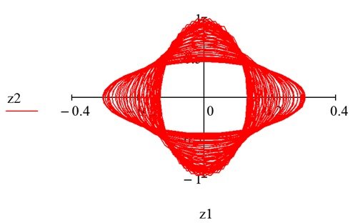
Figure 6 presents the phase portrait illustrating the behavior of \(z2\) against \(z1\), which exhibits a distinct shape due to changes in the eccentricity parameter \(e\).

In Figure 7, the trajectory–time response curves are shown for the parameter values \(u(t) = t\) and \(e = 0.5\). The observed changes result from the combined effects of the eccentricity and the form of the input function. The solid lines represent the numerical solution, while the dashed lines indicate chaotic behavior.

In Figure 8, the velocity–time response curves are presented for the parameter values \(u(t) = t\) and \(e = 0.5\). The solid lines represent the numerical solution, while the dashed lines illustrate the chaotic behavior. The solution also exhibits periodicity, as observed from the relationship between the second solution function values and the corresponding independent variable values.

In Figure 9, the phase portrait illustrates the relationship between \(z2\) and \(z1\), displaying a distinct pattern resulting from variations in both the eccentricity \(e\) and the solution function.

In Figure 10, trajectory-time response curves are presented for the parameter values \(u(t) = t\) and \(e = 0.9\). The observed changes are attributed to the high eccentricity and the nature of the solution function. Solid lines correspond to the numerical solution, while dashed lines indicate chaotic behavior.
In Figure 11, velocity-time response curves are shown for the parameter values \(u(t) = t\) and \(e = 0.9\). The solid lines represent the numerical solution, while the dashed lines indicate chaotic behavior. Additionally, the solution exhibits periodicity based on the second solution function values and the independent variable.
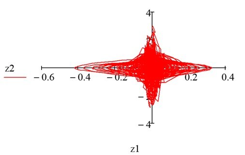
Figure 12 shows the phase portrait illustrating the behavior of \(z2\) versus \(z1\), which exhibits a distinct shape due to variations in the eccentricity \(e\) and the solution function.
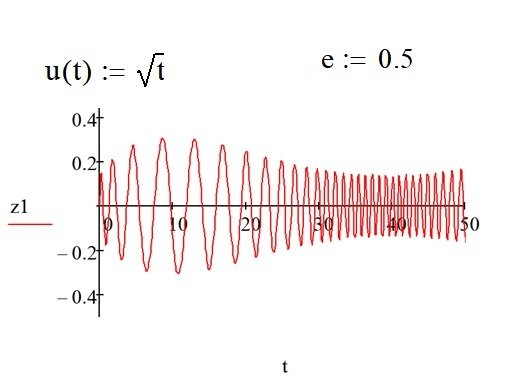
In Figure 13, trajectory-time response curves are presented for the parameter values \(u(t) = \sqrt{t}\) and \(e = 0.5\). The observed changes result from variations in both the eccentricity and the solution function. Solid lines represent the numerical solution, while dashed lines indicate chaotic behavior.
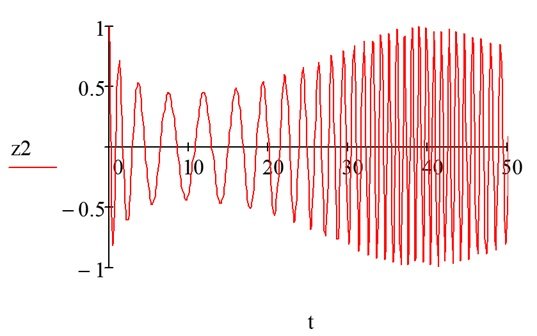
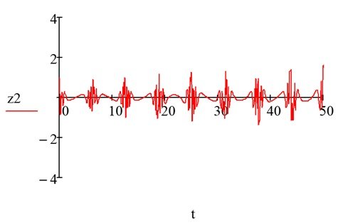
In Figure 14, velocity-time response curves are shown for the parameter values \(u(t) = \sqrt{t}\) and \(e = 0.5\). The solid lines represent the numerical solution, while the dashed lines indicate chaotic behavior. Additionally, the solution exhibits periodicity based on the second solution function values and the independent variable.
In Figure 15, the phase portrait illustrates the behavior of \(z2\) versus \(z1\), exhibiting a distinct shape due to variations in the eccentricity \(e\) and the solution function.
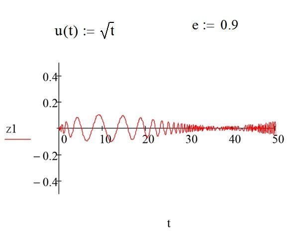
In Figure 16, the trajectory \(z(t)\) is plotted as a function of time, illustrating the variation between the values of the two variables. The solid lines represent the numerical solution, while the dashed lines indicate chaotic behavior.

In Figure 17, velocity-time response curves are presented for the parameter values \(u(t) = \sqrt{t}\) and \(e = 0.9\). The solid lines correspond to the numerical solution, while the dashed lines depict chaotic behavior. Additionally, the solution exhibits periodicity when considering the second solution function values and the independent variable.
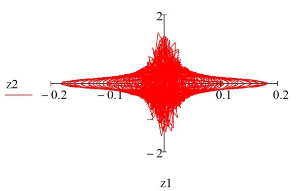
In Figure 18, the phase portrait illustrates the relationship between \(z2\) and \(z1\).
If it is possible to take the primaries in such a way that \(e<0\), then the single oval trajectories will be bifurcated into two oval trajectories by the axis of rotation with a corridor at the neighborhood of the origin.
An approximate solution of the Sitnikov problem has been investigated using the fourth-order Runge-Kutta methods. The various values of eccentricities were obtained which showed the symmetric and periodic nature of the solution in the figures above. This demonstration was done by simulations using MATCAD. The simulations reviews that range of eccentricities can be narrowed down at different values.