
There are a number of mechanisms which can be abstractly defined and are found to be implemented in biology. The best-known is the selectionist mechanism of biological evolution. But that mechanism can be abstractly described and then implemented in non-biological settings as in ‘evolutionary’ or selectionist programs on computers. In that mechanism, a wide variety of different options are randomly generated and then whittled down to a ‘select few’ using some fitness criterion.
Our purpose in this paper is to abstractly describe another ‘dual’ type of mechanism, a generative mechanism, that is also found to be implemented in biology. A generative mechanism can be abstractly described using the graph-theoretic notion of a tree usually pictured upside down with the root at the top and then the branches going downward to eventually terminate in the leaves.
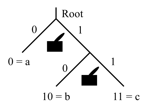
Definition 1. A generative mechanism implements a “code” that determines which branch of a tree is taken as one descends from the root to a specific leaf that was encoded in the code.
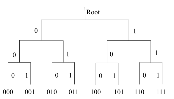
For instance, in Figure 1, reading the three-letter binary codes words from left to right, the code word \(011\) is implemented by taking the \(0\)-branch at the first branching point and then the \(1\)-branch at the next two branching points.1
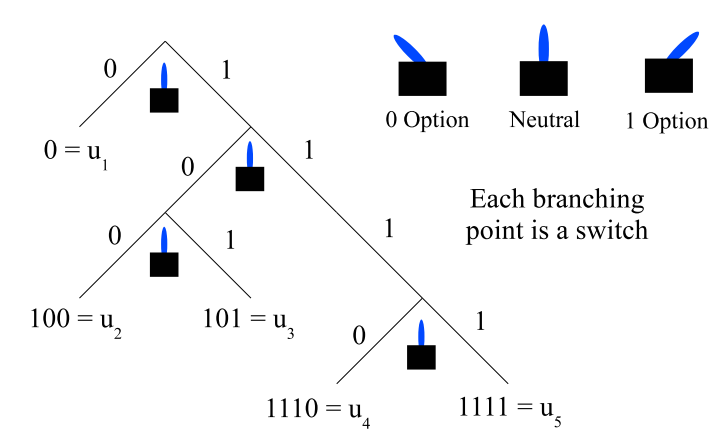
One can think of a code as a hierarchical set of switches. The number of settings on each switch (aside from neutral) is the number of letters in the code alphabet. Each switch determines a branching point in the tree as in Figure 2.
An everyday example of a generative mechanism is the game of 20 questions where a player tries to traverse an implicit tree of binary branching points (yes-or-no questions) to determine the hidden answer at a leaf of the tree. By implementing a code, a generative mechanism navigates down through a diverse set of possible outcomes, represented by the leaves on the tree, to reach a specific outcome or message.
Mathematically, a partition on a set represents one way to differentiate the elements of the set into different blocks. The join with another partition generates a partition with more refined (smaller) blocks that makes all the distinctions of the partitions in the join. Starting from a single block consisting of the set of all possibilities (like the unbranched root of the tree), a sequence of partitions joined together differentiates all the elements of the set ultimately into singleton blocks that are the leaves of the tree. All the (prefix-free) codes of coding theory can be generated in this way and then the codes are implemented in practice to generate the coded outcomes.
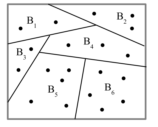
A partition \(\pi=\left\{ B_{1},…,B_{m}\right\}\) is a set of non-empty subsets \(B_{i}\), called blocks, of a universe set \(U=\left\{ u_{1},…,u_{n}\right\}\) that are disjoint and whose union is all of \(U\)—as in Figure 3.
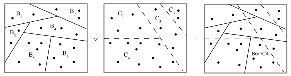
The general idea of a partition is that the elements in the same block are considered indistinct from one another while the elements in different blocks are considered as distinct. Given another partition \(\sigma=\left\{ C_{1},…C_{m^{\prime}}\right\}\), the join \(\pi\vee\sigma\) of the two partitions is the partition whose blocks are the non-empty intersections \(B_{i}\cap C_{i^{\prime}}\) of the blocks of the two partitions. Each partition can also be viewed as an equivalence relation where the equivalence classes are the blocks of the partition. An ordered pair \(\left( u_{i},u_{k}\right)\) of elements of \(U\) in different blocks of a partition \(\pi\) is a distinction or dit of \(\pi\) and the set of all distinctions is the ditset \(\operatorname*{dit}\left( \pi\right) \subseteq U\times U\). The complementary set \(\operatorname*{indit}\left( \pi\right) =U\times U-\operatorname*{dit}\left( \pi\right) =\cup_{j=1}^{m}B_{j}\times B_{j}\) is the set of pairs of elements in the same block of \(\pi\) called indistinctions or indits. The inditset \(\operatorname*{indit}\left( \pi\right)\) is the equivalence relation associated with the partition \(\pi\). Then the intersection or meet of two equivalence relations is the same operation as the join of the two corresponding partitions. That is, since \(\operatorname*{dit}\left( \pi \vee\sigma\right) =\operatorname*{dit}\left( \pi\right) \cup \operatorname*{dit}\left( \sigma\right)\), (where the superscript \(c\) is the complement):
\[\operatorname*{indit}\left( \pi\vee\sigma\right) =U\times U-\operatorname*{dit}\left( \pi\vee\sigma\right) =\operatorname*{dit}\left( \pi\vee\sigma\right) ^{c}=\left( \operatorname*{dit}\left( \pi\right) \cup\operatorname*{dit}\left( \sigma\right) \right) ^{c}% =\operatorname*{dit}\left( \pi\right) ^{c}\cap\operatorname*{dit}\left( \sigma\right) ^{c}=\operatorname*{indit}\left( \pi\right) \cap \operatorname*{indit}\left( \sigma\right),\] using DeMorgan’s law where for any subset \(S\) and \(T\), \(\left( S\cup T\right) ^{c}=S^{c}\cap T^{c}\).
With consecutive joins of partitions (always on the same universe set), the blocks get smaller and smaller until they reach the discrete partition \(\mathbf{1}_{U}\) with the smallest non-empty blocks with are the singletons of elements of \(U\). The least refined partition is the indiscrete partition \(\mathbf{0}_{U}=\left\{ U\right\}\) whose only block is all of \(U\) and it represents the root of the tree that would illustrate the consecutive joins in Table 1 where \(U=\left\{ u_{1}% ,…,u_{5}\right\}\).
| Partitions | Consecutive Joins (tree) | Codes |
|---|---|---|
| \(\{u_{1},u_{2},u_{3},u_{4},u_{5}\}=\mathbf{0}_{U}\) | \(\{u_{1}% ,u_{2},u_{3},u_{4},u_{5}\}=\mathbf{0}_{U}\) | |
| \(\{\{u_{1}\},\{u_{2},u_{3},u_{4},u_{5}\}\}\) | \(\{\{u_{1}\},\{u_{2},u_{3}% ,u_{4},u_{5}\}\}\) | \(0=\) (code for) \(u_{1}\) |
| \(\{\{u_{1},u_{2},u_{3}\},\{u_{4},u_{5}\}\}\) | \(\{\{u_{1}\},\{u_{2}% ,u_{3}\},\{u_{4},u_{5}\}\}\) | |
| \(\{\{u_{1},u_{2}\},\{u_{3},u_{4},u_{5}\}\}\) | \(\{\{u_{1}\},\{u_{2}% \},\{u_{3}\},\{u_{4},u_{5}\}\}\) | \(100=u_{2},101=u_{3}\) |
| \(\{\{u_{1},u_{2},u_{3},u_{4}\},\{u_{5}\}\}\) | \(\{\{u_{1}\},\{u_{2}% \},\{u_{3}\},\{u_{4}\},\{u_{5}\}\}=\mathbf{1}_{U}\) | \(1110=u_{4},1111=u_{5}%\) |
A code is called prefix-free or instantaneous if no code word is the beginning of another code word. All prefix-free code words can be obtained by a sequence of consecutive partition joins in the following manner. The number of letters in the code alphabet is the number of blocks in each partition. All the partitions in the Partitions column of Table 1 (except the indiscrete partition representing the root) have two blocks with the left blocks associated with \(0\) and the right block associated with \(1\). When taking consecutive joins, once a singleton block appears in the Consecutive Joins column, it stays a singleton since it cannot be split any further by further joins.
The code for each \(u_{i}\) in \(U\) is generated in the Partitions column by the sequence of blocks in the binary partitions (ignoring \(\mathbf{0}_{U}\)) containing the element \(u_{i}\), with each block contributing a \(0\) or \(1\) to the code word for the element until it appears in a singleton block in the Consecutive Joins column of Table 1. Then the code word stops so that code word cannot be the prefix for the code word for any other element of \(U\). For instance, consider the element \(u_{2}\) which appears in the \(1\)-block in the first partition \(\{\{u_{1}\},\{u_{2},u_{3},u_{4},u_{5}\}\}\) and then in the \(0\)-block in the next two partitions (in the Partitions column of the table). The element \(u_{2}\) first becomes a singleton in the third row join so tracing its history through the blocks generates the code \(100=u_{2}\).
Corresponding to the generation of a code by consecutive partition joins as in Table 1, one can construct a tree diagram where each branching is accomplished by a partition join and each leaf corresponds to when an element first appears in a singleton. The tree corresponding to Table 1 is the tree in Figure 2.
The most famous code is, of course, the genetic code which is prefix-free so it can be generated by a sequence of partitions. In this case, each partition has four blocks corresponding to the four code letters U, C, A, and G in the code alphabet. For the partitions in Figure 5, which correspond to the (non-indiscrete) partitions in the Partitions column in Table 1, the consecutive joins give all 64 singletons after three branchings or joins so the amino acids have 3-letter code words. The code is redundant since there can be several codes for the same acid.
The circles in Figure 5 trace out the code for Thr4 (one of the code words for Thr, Threonine) which is ACG = Thr4. Note that the order of the partitions counts in the consecutive-joins determination of the genetic codes. A different ordering gives a different code which may not describe the operation of the DNA-RNA machinery to produce a certain amino acid from a given code word.
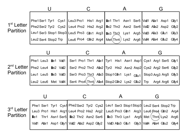
In terms of a tree diagram, the tree would branch four ways at each branching point and there are three levels, so there are \(4^{3}=64\) leaves in the tree. The generative mechanism associated with the genetic code is the whole DNA-RNA machinery that generates the amino acid as the output from the code word as the input. If we abstractly represent the DNA-RNA machinery as that tree with \(64\) leaves, then the given code word tells the machinery how to traverse the tree to arrive at the desired leaf.
Noam Chomsky’s Principles & Parameters (P&P) mechanism ([1]; [2]) for language learning can be modeled as a generative mechanism. Again, we can consider a tree diagram where each branching point has a two-way switch to determine one grammatical rule or another in the language being acquired.
“A simple image may help to convey how such a theory might work. Imagine that a grammar is selected (apart from the meanings of individual words) by setting a small number of switches – 20, say – either “On” or “Off.” Linguistic information available to the child determines how these switches are to be set. In that case, a huge number of different grammars (here, 2 to the twentieth power) will be prelinguistically available, although a small amount of experience may suffice to fix one” [3, p. 154].
And the reference to “20” recalls the game of “20 questions” where the answers to the questions guides one closer and closer to the desired hidden answer. Chomsky uses the Higginbotham model to describe a Universal Grammar (UG) as a generative mechanism.
“Many of these principles are associated with parameters that must be fixed by experience. The parameters must have the property that they can be fixed by quite simple evidence, because this is what is available to the child; the value of the head parameter, for example, can be determined from such sentences as John saw Bill (versus John Bill saw). Once the values of the parameters are set, the whole system is operative. Borrowing an image suggested by James Higginbotham, we may think of UG as an intricately structured system, but one that is only partially ”wired up.” The system is associated with a finite set of switches, each of which has a finite number of positions (perhaps two). Experience is required to set the switches. When they are set, the system functions. The transition from the initial state S0 to the steady state Ss is a matter of setting the switches” [4, p.146].
In the tree modeling of the P&P approach, the relative poverty of linguistic experience that sets the switches plays the role of the code that guides the mechanism from the undifferentiated root state (all switches at neutral) to the final specific grammar represented as a leaf.
“Most important of all, it offered an explanatory model for the empirical analyses which opened a way to meet the challenge of “Plato’s Problem” posed by children’s effortless “yet completely successful” acquisition of their grammars under the conditions of the poverty of the stimulus. This becomes particularly clear if we take the view that parametric variation exhausts the possible morphosyntactic variation among languages and further assume that there is a fı̈nite set of binary parameters. Imposing an arbitrary order on the parameters, a given language’s set of parameter settings can then be reduced to a series of \(0\)s and \(1\)s, i.e. a binary number \(n\)” [5, p. 17].
The binary numbe \(n\) is the code to traverse the tree down to the leaf representing the particular language.
The question about the acquisition of a grammar is a good topic to compare and contrast a selectionist mechanism with a generative mechanism. What would a selectionist approach to learning a grammar look like? A child would (perhaps randomly) generate a diverse range of babblings, some of which would be differentially reinforced by the linguistic environment (e.g., [6]).
“Skinner, for example, was very explicit about it. He pointed out, and he was right, that the logic of radical behaviorism was about the same as the logic of a pure form of selectionism that no serious biologist could pay attention to, but which is [a form of] popular biology – selection takes any path. And parts of it get put in behaviorist terms: the right paths get reinforced and extended, and so on. It’s like a sixth grade version of the theory of evolution. It can’t possibly be right. But he was correct in pointing out that the logic of behaviorism is like that [of naı̈ve adaptationism], as did Quine” [7, Section 10].
As noted, Willard Quine adopts essentially the behaviorist/selectionist account.
“An oddity of our garrulous species is the babbling period of late infancy. This random vocal behavior affords parents continual opportunities for reinforcing such chance utterances as they see fit; and so the rudiments of speech are handed down” [8, p. 73].
“It remains clear in any event that the child’s early learning of a verbal response depends on society’s reinforcement of the response in association with the stimulations that merit the response, from society’s point of view, and society’s discouragement of it otherwise” [8, p 75].
A more sophisticated version of a selectionist model for the language-acquisition faculty or universal grammar (UG) could be called the format-selection (FS) approach (Chomsky, private communication). The diverse variants that are actualized in the mental mechanism are different sets of rules or grammars. Then given some linguistic input from the linguistic environment, the grammars are evaluated according to some evaluation metric, and the best rules are selected.
“Universal grammar, in turn, contains a rule system that generates a set (or a search space) of grammars, {G1, G2,…, Gn}. These grammars can be constructed by the language learner as potential candidates for the grammar that needs to be learned. The learner cannot end up with a grammar that is not part of this search space. In this sense, UG contains the possibility to learn all human languages (and many more). … The learner has a mechanism to evaluate input sentences and to choose one of the candidate grammars that are contained in his search space” [9, p. 292].
After a sufficient stream of linguistic inputs, the mechanism should converge to the best grammar that matches the linguistic environment. Since it is optimizing over sets of rules, this model at least takes seriously the need to account for the choice of rules (rather than just assuming the child can infer the rules from raw linguistic data). Early work (through the 1970s) on accounting for the language-acquisition faculty or universal grammar (UG) seems to have assumed such an approach. The problems that eventually arose with the FS approach could be seen as the conflict between descriptive and explanatory adequacy.
“It was an intuitively obvious way to conceive of acquisition at the time for—among other things—it did appear to yield answers and was at least more computationally tractable than what was offered in structural linguistics, where the alternatives found in structural linguistics could not even explain how that child managed to get anything like a morpheme out of data. But the space of choices remained far too large; the approach was theoretically implementable, but completely unfeasible” [7, Appendix IX].
In order to describe the enormous range of human language grammars, the range of grammars considered would make for an unfeasible computational load of evaluating the linguistic experience. If the range was restricted to make computation more feasible, then it would not explain the variety of human languages. Hence the claim is that the P&P generative mechanism gives a more plausible account of human language acquisition than a behavioral/selectionist approach.2
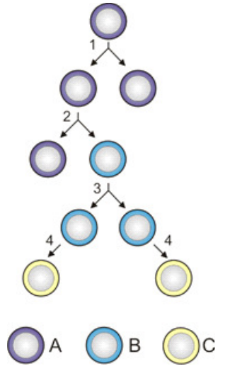
The role of stem cells in the development of an embryo into a full organism can again be modeled as a generative mechanism. The original fertilized egg becomes the stem cell that is the root of the tree. As illustrated in Figure 6, stem cells come in three general varieties: A) the stem cells that can reproduce undifferentiated copies of themselves, B) the stem cells that can reproduce but can also produce a somewhat differentiated cell, and C) a specialized differentiated cell. Each branching point in a tree has a certain number of possible leaves or terminal types of cells beneath it in the tree. In a division (#1) of an A-type cell, each of the resulting A-type cell could have a full set of leaves beneath it. But when it splits (#2) into another A-type cell and a B-type cell, then the B-cell has a restricted number of leaves beneath it. The B-type cells can split (#3) in two, and finally when a B-type cell gives rise (#4) to a specific C-type of cell, that is a terminal branch, i.e., a leaf, in the tree.
The codes that inform the progress through the tree are not fully understood, but apparently the positional epigenetic information in the developing embryo provides the information about the next development steps. In general terms,
“[t]hat model harks back to the “developmental landscape” proposed by Conrad Waddington in 1956. He likened the process of a cell homing in on its fate to a ball rolling down a series of ever-steepening valleys and forked paths. Cells had to acquire more and more information to refine their positional knowledge over time — as if zeroing in on where and what they were through “the 20 questions game,” according to Jané Kondev, a physicist at Brandeis University” [10].
Again, the reference to the game of 20 questions reveals the common generative mechanism of traversing a tree from the root to a specific leaf.
There is a long tradition in biological thought of juxtaposing selectionism, associated with Darwin, with instructionism, associated with Lamarck ([11]; [12]). In an instructionist or Lamarckian mechanism, the environment would transmit detailed instructions about a certain adaptation to an organism, while in a selectionist mechanism, a diverse variety of (perhaps random) variations would be generated, and then some adaptations would be selected by the environment but without detailed instructions from the environment. The discovery that the immune system was a selectionist mechanism [14] generated a wave of enthusiasm, a “Second Darwinian Revolution” [15], for selectionist theories [16].
In his Nobel Lecture [17], Niels Jerne even tried to draw parallels between Chomsky’s generative grammar and selectionism. One of the distinctive features of a selectionist mechanism is that the possibilities must be in some sense actualized or realized in order for selection to operate on and differentially amplify or select some of the actual variants while the others languish, atrophy, or die off. In the case of the human immune system, “It is estimated that even in the absence of antigen stimulation a human makes at least \(10^{15}\) different antibody molecules—its preimmune antibody repertoire.” [18, p. 1221].
In Chomsky’s critique of a selectionist theory of universal grammar, he noted the computational infeasibility of having representations of all possible human grammars in order for linguistic experience and an evaluation criterion to perform a selective function on them. The analysis of Chomsky’s P&P theory as a generative mechanism instead suggests that the old juxtaposition of “selectionism versus instructionism” is not the most useful framing for the study of biological mechanisms.
The discovery of the genetic code and DNA-RNA machinery for the production of amino acids powerfully showed the existence of another biological mechanism, a generative mechanism, that is quite distinct from a selectionist mechanism. The examples of Chomsky’s P&P theory of grammar acquisition and the role of stem cells in embryonic development provide more evidence of the importance of generative mechanisms.
To better illustrate these two main types of biological mechanisms, it might be useful to illustrate a selectionist and a generative mechanism in solving the same problem of determining one among the \(8=2^{3}\) options considered in Figure 1. The eight possible outcomes might be represented as: \(|000\rangle ,|100\rangle,|010\rangle,|110\rangle,|001\rangle,|101\rangle,|011\rangle ,|111\rangle.\)
In the selectionist scheme, all eight variants are in some sense actualized or realized in the initial state \(S_{0}\) so that a fitness criterion or evaluation metric (as in the FS scheme) can operate on them. Some variants do better and some worse as indicated by the type size in Figure 7.
The “unfit” options dwindle, atrophy, or die off leaving the most fit option \(|010\rangle\) as the final outcome.
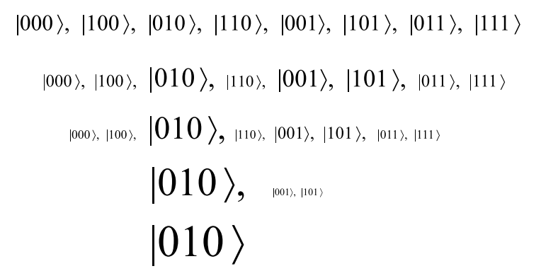
With the generative mechanism, the initial state \(S_{0}\) (the root of the tree) is where all the switches are in neutral, so all the eight potential outcomes are in a “superposition” (between left and right) state indicated by the plus signs in the following Figure 8.

The initial experience or first letter in the code sets the first switch to the \(0\) option which reduces the state to \(|000\rangle+|001\rangle +|010\rangle+|011\rangle\) (where the plus signs in the superposition of these options indicate that the second and third switches are still in neutral). Then subsequent experience sets the second switch to the \(1\) option and the third switch to the \(0\) option. Thus, we reach the same outcome \(|010\rangle\) as the final outcome in the two models but by quite different mechanisms. Note that the generative mechanism ‘selects’ or determines a specific outcome but that does not make it a ‘selectionist’ mechanism.
While our focus is on biological mechanisms, calling the root state a “superposition” is not an accident. In quantum mechanics, a (projective) measurement starts with a superposition pure state represented by the normalized incidence matrix for an equivalence relation, i.e., a density matrix. Then the observable being measured is represented by the vector space version of a partition, namely the direct-sum decomposition consisting of the eigenspaces of the observable. The measurement turns the pure state into the probabilistic mixed state density matrix representing the intersection of the two corresponding equivalence relations where that operation is called the “Lüders mixture operation.” Then the determination of a particular state like \(\left\vert 010\right\rangle\) is the probabilistic “ reduction of state” (or so-called “collapse of the wave packet”) ([19], [20]). In the example, the superposition of the eight states is turned by the measurement into a probabilistic mixture or ‘lottery’ of the states (e.g., probability \(\frac {1}{8}\) each) and then the ‘lottery’ yields one of the specific probabilistic outcomes such as \(\left\vert 010\right\rangle\).
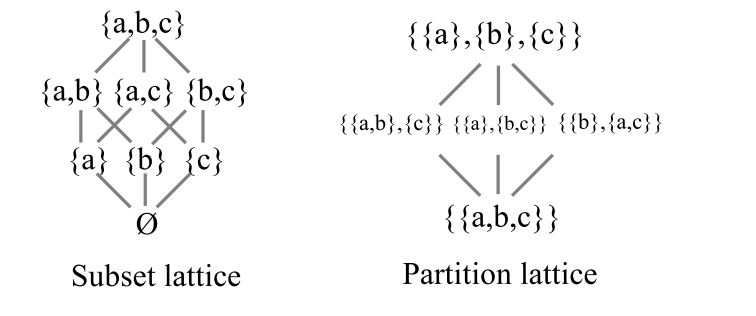
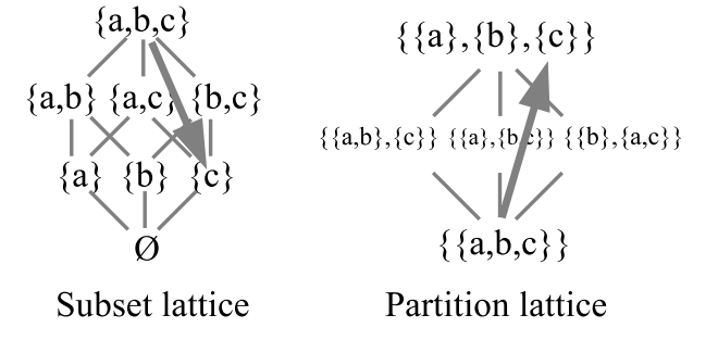
There is another way to contrast a selective and generative mechanism, namely duality [21]. In logic [22], there are two principal lattices, the lattice of subsets of a universe \(U\) and the lattice of partitions on \(U\). They are the two dual lattices because the category-theoretic dual of the notion of a subset (or more generally, a subobject or ‘part’) and the notion of a partition or equivalence relation (or quotient object). “The dual notion (obtained by reversing the arrows) of ‘part’ is the notion of partition” [23, p. 85].
For \(U=\{a,b,c\}\), the two lattices are pictured in Figure 9. The lines connecting the subsets in the subset lattice is just the set inclusion relation and the lines connecting the partitions in the partition lattices is the refinement relation (i.e., \(\pi\) is more refined that \(\sigma\) if the blocks of \(\pi\) can be obtained by chopping up the blocks of \(\sigma\)).
A selective mechanism to determine \(a\), \(b\), or \(c\) from \(U\) would start with all the actual elements (top of the subset lattice) since an alternative has to actualized before a fitness or evaluation criterion criteria can narrow the set of actualities down to the selected one.
A generative mechanism starts with the indiscrete partition \(\mathbf{0}% _{U}=\{\{a,b,c\}\}=\{U\}\) (at the bottom of the partition lattice) where all the elements are only potential outcomes not distinguished from each other. Then distinctions are made, as represented by consecutive partition joins, until an element is fully distinguished from the other elements (i.e., appears as a singleton) which completes the code word that will determine that element.
The dual mechanisms for determining \(c\) are given in Figure 10.
The selectionist and generative mechanism are, according to this analysis, the only two mechanisms to go in Nature from the “many” to the “one.”
In the generative case, a coding scheme to code each element by partition joins is given in Table 2.
| Partitions | Consecutive joins | Codes |
|---|---|---|
| \(\{\{a,b,c\}\}=\mathbf{0}_{U}\) | \(\{\{a,b,c\}\}=\mathbf{0}_{U}\) | |
| \(\{\{a\},\{b,c\}\}\) | \(\{\{a\},\{b,c\}\}\) | \(0=a\) |
| \(\{\{a,b\},\{c\}\}\) | \(\{a\},\{b\},\{c\}\}=\mathbf{1}_{U}\) | \(10=b,11=c\) |
The tree diagram for the Table 2 code implemented by the switches to give \(c\) is given in Figure 11.
Finally, it should be mentioned that there is an intimate connection between the tree diagrams representing generative mechanisms and information theory ([24]; [25]). One can imagine a marble rolling down from the root to one of the leaves where its path was probabilistically determined at each branching point by a set of probabilities. The simplest assumption on a binary tree is a half-half probability of the marble taking each branch. From each leaf, there is a unique path from the root to the leaf and the product of the probabilities along that path gives the probability of reaching that leaf. With those assumptions for the tree of Figure 1, each leaf has probability \(1/2^{3}=1/8\). Then the Shannon entropy of that probability distribution \(p=(p_{1}% ,\ldots,p_{m})\) is:
\[H(p)=\sum_{i}p_{i}\log_{2}(1/p_{i})=8\times1/8\times\log_{2}(1/(1/8))=\log _{2}(2^{3})=3,\] and the logical entropy is:
\[h(p)=1-\sum_{i}p_{i}^{2}=1-8\times(1/8)^{2}=1-1/8=7/8.\]
In this simple example, the Shannon entropy is the average number of binary partitions (bits) needed to distinguish all the leaves on the tree (“messages”). The logical entropy always has the interpretation that on two independent trials, there will be different outcomes. In this case, that is the probability that on two independent rolls of a marble, it will end up at different leaves. Since all the leaves are equiprobable, it is simply the probability that the second marble took a different path (than on the first trial), i.e., \(1-1/8=7/8\). Moreover, in this simple example of equiprobable leaves, the two entropies are related by \(H\left( p\right) =\log_{2}\left( \frac{1}{1-h\left( p\right) }\right)\).
With the same half-half branching probabilities for Figure 11, the leaf probabilities are \(\Pr(a)=1/2\) and \(\Pr(b)=\Pr(c)=1/2\times1/2=1/4\). Then the Shannon entropy is:
\[H(p)=1/2\times\log_{2}(1/(1/2)+2\times1/4\times\log_{2}% (1/(1/4))=1/2+(1/2)\times2=3/2,\] which is, in this simple case, the average length of the code words for the leaves. The logical entropy is:
\[h(p)=1-(1/2)^{2}-2\times(1/4)^{2}=1-1/4-1/8=5/8,\] which is always the probability that on two rolls, the marble will end up at different leaves.
Tracing down a code tree from the root to the desired message generates the code for that message on the sending side of a communications channel, and then implementing the received code on the receiving side of the channel will generate the received message. In the case of the biological examples (genetic code, generative grammar, and embryonic development), the creation of the codes is a matter of deep evolutionary history, so the focus of study is usually on how those generative mechanisms implement codes to give specific outcomes.