
Economic systems characterised by interactions among capital investment, productivity, wage shares, and employment rates, are complex and dynamic [1, 2]. It is therefore essential to comprehend these interactions to develop economic strategies and policies that work. Traditionally applied in ecology, predator-prey models are one type of mathematical modelling that can be used to explore these dynamic interactions [3, 4]. The predator-prey concept that underpins the Class Struggle Model offers an analogy for economic dynamics, particularly when it comes to linkages between wage share and employment. The Lotka-Volterra equations are modified in the Class Struggle Model to explain the cyclical relationships between capitalists (employers) and workers [5, 6]. In the Class Struggle Model, employment rate and wage share oscillate, mirroring the underlying conflicts and negotiation between capital and labour over economic output. This behaviour is comparable to the population dynamics of predators and their prey.
The purpose of this study is to model the employment and wage dynamics in Ghana’s economy from 1990 to 2008 using a predator-prey approach of Goodwin’s theoretical framework. Attempt is made to represent the interaction between wage share and employment rate by developing a system of first-order ordinary differential equations. The study also attempts to simulate the dynamic behaviour between employment rate and wage share, assess the Model’s robustness through analytical and sensitivity analyses, and carry out qualitative analysis using phase portraits and vector field plots. The application of this Theoretical Model to empirical data from Ghana provides insights into the specific economic context of the Ghana and contributes to the understanding of employment-wage dynamics. The period 1990 – 2008, according to [7] and [8], Ghana’s economy is significant because various economic reforms and policies, which have implications for labour market dynamics and income distribution were implemented in Ghana.
Generally, a model is a simplified representation of the real world. Subsequently, [9] describes mathematical models as the act and science of constructing equations or formulae based on quantitative description of real phenomena for gaining insight and making predictions into real phenomena. Similarly, economic models are simplified representations of economic processes [10]. Deducing from [10], mathematical equations, graphs, and diagrams are used to describe, explain, and predict economic phenomena relating to microeconomic, macroeconomic, econometric, and game theoretic models, which focus on consumers, firms, markets, and other economic matrices such as GDP, inflation, interest rates, and un/employment. Imperatively, the goal in modelling is not to produce a model that is correct but rather to elegantly describe and predict observations. Be it a simple or complex model, the process of economic modelling is systematic. Among several of such of such processes [11] enumerated six systematic steps as defining the variables, specifying functions (identities and equations which show how the variables are related), choosing a solution principle, solving the model, interpreting the solution, and analysing perturbations of the solution.
Predation models, traditionally used in ecology to describe interactions between predator and prey species, have found a valuable place in economic modelling, particularly in the study of dynamic and cyclical interactions in economies [3, 4]. Foundational predation models include Godwin’s Model and the Class Struggle Theory.
As explained [3, 4], Godwin’s model applied Lotka-Volterra predator-prey equations in two parts to describe the cyclical interaction between the prey and predator variables. The change in prey population through time \(\frac{\mathrm{dV}}{\mathrm{dt}}=\mathrm{rV\ -\ (aV)P\ }\), \(r>0\) and \(a>0\) and the change in predator population size through time \(\frac{\mathrm{dP}}{\mathrm{dt}}=(\mathrm{bV)P\ -\ dP\ }\), \(b>0\) and \(d>0\). The efficiency factor, b, measures how well the predator converts food into offspring. A less efficient predator will expend more of its energy on maintenance than on reproduction compared to an efficient predator. This model is simplistic because it assumes exponential growth of prey, and a predator can eat as many preys as it can catch – that is, it never gets full! The basic model gives several important results such as: that predator and prey populations will oscillate through time. If the predator and prey populations are roughly in balance (populations rise and fall in the short-term, but the long-term average size of the populations does not change) then several more results accrue. That the predator abundance depends more on the prey growth rate \((r)\) than on its own death rate \((d)\), whereas prey abundance is controlled more by predator death rate than by its own growth rate. That a lower feeding rate \((a)\) for each predator will result in a higher prey population but also more predators because more predators will be recruited to maintain the overall predation rate on the prey population. That if the predators increase their efficiency \((b)\), and produce more new predators from captured prey, prey abundance decreases, but predator abundance is unaffected.
A more realistic model of predation incorporates logistic growth for the prey populations, and rather than assume that predation rate simply related to prey density, it incorporates a predator satiation factor [12, 13]. When the preys are very abundant, a predator can no longer continue to increase its feeding rate because it becomes full. The model is composed of the simultaneous equations \(\frac{\mathrm{dV}}{\mathrm{dt\ }}=\mathrm{r}\left(\mathrm{1-}\frac{\mathrm{V}}{\mathrm{K}}\right)\mathrm{V-c}\left(\mathrm{1-}{\mathrm{e}}^{-\frac{av}{c}}\right)\mathrm{P}\) and \(\frac{\mathrm{dP}}{\mathrm{dt}}=bc\left(\mathrm{1-}{\mathrm{e}}^{-\frac{av}{c}}\right)P-dP\). With this model, both oscillations and stable coexistence are possible. Dawed (2014) extended the model by considering the predator’s population growth, showing that it could converge to a finite positive limit, 0, or diverge to infinity. Subsequently, the prey carrying capacity, K, is important in controlling the type and stability of the predator-prey interaction. At low prey carrying capacity, both predator and prey populations remain steady with only small fluctuations in each. Oscillations occur if K is large enough, and is partly due to the destabilising effects of satiation, which allow the prey to “get away” from the predators for a while until they approach their own carrying capacity. Predator numbers, on the other hand, still increase until they begin to regulate the prey again and prey abundance decreases. As a result, predator numbers fall, and the cycle begins again. At higher K, the oscillations can get so large that one or other population goes extinct. There is an optimum feeding rate that maximizes the predator population size. Too high a predation rate, and the prey are overexploited and the resource will become depleted. Predator population size maximised when the prey population equals half the carrying capacity level.
The Class Struggle Theory grounds Goodwin’s model in Marxian economic theory [14], where the capital-labour dynamic is akin to a predator-prey relationship, reflecting the struggle between capitalists (owners of production) and workers over the distribution of economic output. Capitalists possess profit maximising interest whereas workers who do not own the means of production, must trade-off their labour to secure wages to survive. The Class Struggle Theory as explored by [15], [16], and [17], provides a framework for exploring the dynamics of capitalism and the conflicts between different social classes, and a framework for analysing economic inequality and labour relations. The theory’s essential set-up begun with two classes of income recipients wage-earning workers, and profit-earning capitalists. For good a measure, exogenous growth components – namely, labour supply growth and productivity growth were introduced [18]. Two differential equations which reflect the growth in labour employment \((\mu )\) and wage share \((u)\) respectively based on the predator-prey equations are formed: \(d\mu \ /dt\ =\ [1/v\ -\ (\theta +\ n)\ -\ u/v]\mu\) and \(du/dt\ =\ [-\ (\propto +\theta )\ +\beta \mu ]u\).
Three methods for solving ordinary differential equations exist – The Analytical, Qualitative and Numerical approach [19]. The analytical approach includes separation of variables, method of undetermined coefficients, variation of parameters, exact differential equations, integrating factors and series solutions of differential equations. For nonlinear differential equations, common methods for quantitative analysis include the examination of any conserved quantities especially in Hamiltonian systems, examination of dissipative quantities, linearization, change of variables, bifurcation, and perturbation methods. The qualitative approach involves using geometry for example, direction/vector fields to give an overview of the behaviour of the model. As explained by [20], although qualitative methods do not give precise values of the solution, they aid in determining long-term behaviour of solutions. Numerical approach is the computer approximation to the solutions. Computer codes and programmes such as Runge-Kutta methods, MATLAB ODE solvers, and Euler methods are some examples. Nevertheless, literature [21, 22] show that the application of these methods on nonlinear differential equations may result in indeterminism, multi-stability, and periodic/chaotic oscillation situations.
The assumptions relate to the Goodwin’s class struggle model, which is akin to the predator prey model [19, 23].
A closed economy with government activity assumed. Only two factors of production- labour and capital exist for production. The owners of investment/capital are the capitalist and wage earners are workers. The idea is capitalist save all their income such that savings become the prerequisite for investment. However, workers consume all their incomes (there are no savings out of wage income).
Output levels determine employment \(\left(a=\frac{Q}{L}\ \Longrightarrow L=\frac{Q}{a}\right)\).
Employment levels determine the rate of change of wages. When real wages increase less than labour productivity, profit share increases, and investment levels rise. This leads to higher demand for labour and workers get more power to seek for high wages.
The differential equation of the rate of change of wages determines wages \(\left(\frac{dw}{dt}=w\right)\).
Output less the wage bill determines profit, and it is automatically saved \(\left(s=Q-Lw\ \Longrightarrow s=1-y\right)\).
Savings determines investment \(\left(I=s,\ \Longrightarrow I=k(s)\right)\).
Capital investment determines output as advocated by Harrod (1900-1978) that investment increases output, and output induces investment \(\left(Q=\frac{k}{v}\ \Longrightarrow v=\frac{k}{Q}\right)\).
An exponential/natural growth in the labour force and labour productivity is assumed \(\left(\frac{dN}{dt}=N\beta \ \Longrightarrow N\left(t\right)=N_0e^{\beta t}\mathrm{\ \ and\ }\frac{da}{dt}=a\propto \ \Longrightarrow a\left(t\right)=a_0e^{\propto t}\right)\)
\(L\equiv\) Labour (workers); \(Q\equiv \ \)Output (real GDP); \(k\equiv\) Capital; \(N\equiv\) Labour force
\(x={L}/{N}\equiv\) Labour employment rate; \(wL\equiv\)Wage bill; \(v={k}/{Q}\equiv\) Capital-output ratio
\(a={Q}/{L}\equiv\) Average labour productivity; \(y={wL}/{Q}={w}/{a}\equiv\) Wage share returns on capital investment.
From \(x=\frac{L}{N}\), the differential equation of the rate of employment is derived as: \[\begin{aligned} \label{eq1} \frac{dx}{dt}=&\frac{d}{dt}\left(\frac{L}{N}\right),\nonumber\\ \frac{dx}{dt}=&\frac{1}{N}\frac{d}{dt}L+L\frac{d}{dt}\left(\frac{1}{N}\right),\nonumber\\ \frac{dx}{dt}=&\frac{1}{N}\frac{d}{dt}\frac{Q}{a}+L\left(\frac{-1}{N^2}\right)\frac{d}{dt}N ,\nonumber\\ \frac{dx}{dt}=&\frac{1}{N}\left[\frac{1}{a}\frac{d}{dt}Q+Q\left(\frac{-1}{a^2}\right)\frac{d}{dt}a\right]-\frac{L}{N}\frac{1}{N}\frac{d}{dt}N ,\nonumber\\ \frac{dx}{dt}=&\frac{1}{N}\left[\frac{1}{a}\frac{d}{dt}\left(\frac{K}{v}\right)-\left(\frac{Q}{a}\right)\frac{1}{a}\frac{d}{dt}a\right]-x\beta , \nonumber\\ \frac{dx}{dt}=&\frac{1}{N}\left[\frac{1}{a}\frac{I}{v}-\left(\frac{La}{a}\right)\propto \right]-x\beta ,\nonumber\\ \frac{dx}{dt}=&\frac{1}{N}\left[\frac{1}{a}\frac{Q-Lw}{v}\right]-x\propto -x\beta ,\nonumber\\ \frac{dx}{dt}=&x\left[\frac{1-\frac{w}{a}}{v}\right]-x\propto -x\beta ,\nonumber\\ \frac{dx}{dt}=&x\left[\frac{1-y}{v}-\propto -\beta \right],\nonumber\\ \mathrm{\therefore }\frac{dx}{dt}=&\left[\frac{1}{v}-\left(\propto +\beta \right)-\frac{y}{v}\right]x, \end{aligned} \tag{1}\] where \(y\equiv worker's\ share,\ 1-y\equiv capitalist's\ share.\) Phillips curve [24] depicts a positive relation between employment rate and real wage. Assuming a linear Phillips’ curve representation of wage growth, then, \(\dot{w}=(-\gamma +\rho x)w\). For \(\gamma\), the intercept and \(\rho\), the slope of the Phillips curve.
Now from \(y=\frac{w}{a}\), the differential equation of the rate in wage share is obtained as: \[\begin{aligned} \label{eq2} \frac{dy}{dt}=&\frac{d}{dt}\left(\frac{w}{a}\right),\nonumber\\ \frac{dy}{dt}=&\frac{1}{a}\frac{d}{dt}w+w\frac{d}{dt}\left(\frac{1}{a}\right),\nonumber\\ \frac{dy}{dt}=&\frac{1}{a}\left(\left(-\gamma +\rho x\right)w\right)+w\left(\frac{-1}{a^2}\right)\frac{d}{dt}a, \nonumber\\ \frac{dy}{dt}=&\frac{w}{a}\left(-\gamma +\rho x\right)-\frac{w}{a}\left(\frac{1}{a}\right)a\propto , \nonumber\\ \frac{dy}{dt}=&y\left(-\gamma +\rho x\right)-y\propto, \nonumber\\ \frac{dy}{dt}=&\left[\rho x-\gamma -\propto \right]y, \nonumber\\ \therefore \frac{dy}{dt}=&\left[\rho x-\left(\gamma +\propto \right)\right]y. \end{aligned} \tag{2}\]
Eqs. (1) and (2) combined bring to fore the Goodwin’s class struggle (real employment-real wage cycle) model. The model for this project therefore is a system of first-order ordinary predator-prey nonlinear differential equations in employment rate represented by \(x\) and the wage share represented by \(y\).
\[\begin{aligned} \label{eq3} \frac{dx}{dt}=&\left[\frac{1}{v}-\left(\alpha +\beta \right)-\frac{y}{v}\right]x, \nonumber\\ \frac{dy}{dt}=&\left[\rho x-\left(\gamma +\alpha \right)\right]y. \end{aligned} \tag{3}\]
Model (3) is analogous to the Predator-prey model in various ways; \(y\) corresponds to workers share of the output [(\(1-y)\) is the capitalist share of the output] and \(x\) is the employment rate. In reference to Eqs. (1) and (2), workers are identified with the predators and the capitalist, the prey. From Eq. (1), the employment rate increases more quickly the larger the capitalist’s share and from Eq. (2), the smaller the employment rate, the more rapid increase in the capitalist share. This phenomenon is akin to the Predator-prey relation where the predator population grows faster the more the prey population and the prey population grows faster the smaller the predator population.
The data for this research were sourced from the websites of creditable national and international agencies. These agencies include the Finance and Economic Planning ministry, the Bank of Ghana, the Ghana Statistical Service, the Trading Economics and the Labour Statistics Database. A summary of the data is presented in the Appendix. Consequently, the study applies the Goodwin’s class struggle model, which is a variant of the predator prey model to test the theoretical hypothesis empirically using annual data from 1990 to 2008 of Ghana.
Figure 1 shows the average growth rates in real GDP, labour, and capital formation.

As depicted in Figure 1, the growth rate in real GDP was characterised by cyclical fluctuations comparable to economic studies [25, 26]. The average rate of growth in real GDP was 4.9% with an average GDP of \(GH\)/2733.8 million over the 19-year period under review. For the growth rate in the labour market (Figure 1), there was a steady growth over the period 1990 to 2008. The average employment rate of growth recorded was 3.4% higher than the population growth rate of 2.5% and labour force of 3.2% over the same period. The average labour employed was 7,477. The model which approximately described the labour force from 1990 to 2008 was \(N\left(t\right)=5715.363e^{0.03280318\boldsymbol{t}}\). An average \(GH\mathrm{\textrm{{C}}}\) 684.8 million capital investment showed an average growth rate of 12.3% in gross capital formation (Figure 1) although characterised with unpredictable fluctuations. Although the graph of labour productivity (Figure 1) compared well to the graph of a fourth-degree polynomial when plotted with MATLAB rather than the exponential growth model, the exponential growth model result \(a\left(t\right)=0.047304e^{0.08538687t}\) was used per the initial assumptions. Figure 1 further showed the share of labour and capital formation to the real GDP. Arguably, labour share (employee compensation-GDP ratio) was higher than capital share (capital-output ratio) an indication that the national economy was more of labour intensive than capital intensive.
Inferred from Model (3), which relates the employment rate (prey) to the wage share (predator) variables, \(v=\frac{k}{Q}=0.2\) is the average capital output ratio over the period, \(\alpha =0.08538687\) is exponential growth rate of labour productivity, \(\beta =0.03280318\) is also the exponential rate of labour force, which according to [18] could act as exogenous growth components to assure a good measure. Using TI 89 Titanium calculator to fit Phillips’ linear curve (Hardwick et al., 1994), \(\dot{w}=-\gamma +\rho x\), on the real wage \((w)\) – employment rate \((x)\) relationship produced \(\gamma =4.24153481\ \)and \(\ \rho =5.13796143\). Substituting the values of the constants in to the system 4.1 and simplifying produce
\[\begin{aligned} \label{eq4} \frac{dx}{dt}=&4.881880995x-5xy \nonumber\\ \frac{dy}{dt}=&5.12796143xy-4.32692168y. \end{aligned} \tag{4}\]
With employment level (Model 4), if wage share vanishes, then \({dx}/{dt}=4.881880995x\). Solving for \(x\) at time \(t=0\), gives \(x\left(t\right)=0.945e^{4.881880995t}\). Thus, as wage share goes to zero, employment rate increases infinitely at an exponential rate of \(4.881880995\). Similarly, if employment rate goes to zero as in wage share equation (Model 4), then solving for \(y\) at time \(t=0\), \(y\left(t\right)=0.0665462e^{-4.32692168t}\). Hence, as employment rate vanishes, the wage share equally goes to zero exponentially at the rate \(4.32692168\).
From Model (4), the right-hand side of the model vanish at \(x=0\ \)and\(\ y=0\). Thus, the constant function \(x\left(t\right)\equiv 0\ \)and \(y(t)\equiv 0\) is an equilibrium solution to Model (4). Also, by equating Model (4) to zero, another set of equilibrium point is derived. That is \(x=0.84214756\) and \(y=0.976376199\) is also an equilibrium solution when \(\dot{x}=0\) and \(\dot{y}=0\). Thus, the equilibrium points are \(\left(0,0\right)\) and\(\ (0.84214756\mathrm{\ },0.976376199)\). The point \((0,0)\), is an uninteresting situation where employment rate and labour wage share do not constitute the economic parameters determining the dynamics of economic growth and the initial assumption that only labour and capital exist for production is defeated [19]. The second nontrivial solution \((0.84214756\mathrm{\ },0.976376199)\) indicates that both employment rate and wage share maintain a unique value. The question of whether this solution is feasible or that it is a stable equilibrium is a concern for this study. Quantitative and qualitative approaches were used to examine the nature of the equilibrium points.
This section presents the analytic solution to Model (3). To do this involved determining the stability of the model by linearization.
By letting \(\dot{x}=F\left(x,y\right)\ \)and\(\ \dot{y}=G(x,y)\), we have \[\begin{aligned} F\left(x,y\right)=&4.881880995x-5xy,\\ G\left(x,y\right)=&5.13796143xy-4.32692168y. \end{aligned}\]
Finding the Jacobian \(J(x,y)\), and linearising the Model (3) near the equilibrium points, \[J\left(x,y\right)=\left[ \begin{array}{cc} 4.881880995-5y & -5x \\ 5.13796143y & 5.13796143x-4.32692168 \end{array} \right]\] \[\mathrm{\Longrightarrow } J\left(0,0\right)=\left[ \begin{array}{cc} 4.881880995 & 0 \\ 0 & -4.32692168 \end{array} \right]\]
The approximation of the system in the neighbourhood of \((0,0)\).
For \[A=\left[ \begin{array}{cc} 4.881880995 & 0 \\ 0 & -4.32692168 \end{array} \right],\] and using the relation \(\left|A-\leftthreetimes I\right|=0\), the eigenvalues in terms of \(\leftthreetimes\) based on the characteristic polynomial \({\leftthreetimes }^2-0.55488827\leftthreetimes -21.12320931=0\), are determined producing \({\leftthreetimes }_1=-4.32692168\ \mathrm{and}\ {\leftthreetimes }_2=4.88180995\). Since the eigenvalues exhibit the characteristics \({\leftthreetimes }_1<0<{\leftthreetimes }_2\), an unstable saddle around the trivial equilibrium \((0,0)\) conclusion can be made (Williamson, 1997). Deductively, as \(t\) increases, the solution paths will initially move in towards the equilibrium solution \((0,0)\) and then, move away eventually from the equilibrium point \((0,0)\) [19].
Determining the behaviour of Model (4) at the non-zero equilibrium \((0.84214756\mathrm{\ },0.976376199)\) involves \[J(0.84214756\mathrm{\ },0.976376199)=\left[ \begin{array}{cc} 0 & -4.21073780 \\ 5.01658325 & 0 \end{array} \right].\]
The approximation of the system in the neighbourhood of \((0.84214756\mathrm{\ },0.976376199)\).
For \[A=\left[ \begin{array}{cc} 0 & -4.21073780 \\ 5.01658325 & 0 \end{array} \right],\] and using the relation \({\leftthreetimes }^2+21.12351672=0\) to determine the eigenvalues, \({\leftthreetimes }_1={-4.59603272}_i\ and\ {\leftthreetimes }_2={4.59603272}_i\). Since both eigenvalues are purely imaginary (complex and conjugate, their real part equalling zero), the system linearised about the equilibrium \((0.84214756\mathrm{\ },0.976376199)\) is a centre. However, as purely eigenvalues on the borderline situation, the linearization stability test is inconclusive [19]. It turns out that the system is a conservative system.
Consequently, finding a corresponding first integral and solving the emerging auxiliary equation of Model (4) gives \(I\left(x,y\right)=4.881880995{\mathrm{ln} \left|y\right|-5y+4.32692168{\mathrm{ln} \left|x\right|\ }-\ }5.13796143x=C\) indicative that the solutions to Model (4) must stay on the level of \(I(x,y)\).
Also \[\mathrm{\nabla }I=\left( \begin{array}{c} \frac{4.32692168}{x}-5.13796143 \\ \frac{4.881880995}{y}-5 \end{array} \right).\]
Hence, \(\mathrm{\nabla }I\left(0.84214756\mathrm{\ },0.976376199\right)=0\), which is an indication that the second equilibrium is a critical point. Moreover, the Hessian matrix \(H\) of a real-valued function \[{\mathrm{H=}\mathrm{\nabla }}^2I=\left[ \begin{array}{cc} \frac{-4.32692168}{x^2} & 0 \\ 0 & \frac{-4.881880995}{y^2} \end{array} \right],\] is negative definite (H has both eigenvalues negative) and hence, \({(0.84214756\mathrm{\ },0.976376199)}^T\) is a strict local maximum of the first integral \(I(x,y)\) [19]. Thus, the equilibrium \((0.84214756\mathrm{\ },0.976376199)\) is a stable centre indeed.
More so, the non-zero eigenvectors \({\mu }^{\left(1\right)}=\left[ \begin{array}{c} 4.21073780 \\ {4.59603272}_i \end{array} \right]\) and \({\mu }^{\left(2\right)}=\left[ \begin{array}{c} 4.21073780 \\ {4.59603272}_i \end{array} \right]\) corresponding to the eigenvalues \({\leftthreetimes }_1={-4.59603272}_i\) and\(\ {\leftthreetimes }_2={4.59603272}_i\) reflecting the equilibrium point \((0.84214756\mathrm{\ },0.976376199)\) was found.
At this stage, emphasising \({\leftthreetimes }_2\) and \({\mu }^{\eqref{eq2}}\) simultaneously, the solution of Model (4) is obtained as \[\left( \begin{array}{c} x(t) \\ y(t) \end{array} \right)=e^{{4.59603272}_i\boldsymbol{t}}\left( \begin{array}{c} 4.21073780 \\ -{4.59603272}_i \end{array} \right).\]
Appling Euler’s formula \(e^{i\theta }=Cos\theta +iSin\theta\), \[\left[ \begin{array}{c} x\left(t\right) \\ y\left(t\right) \end{array} \right]=\left[Cos\left(4.59603272t\right)+iSin\left(4.59603272t\right)\right]\left[ \begin{array}{c} 4.21073780 \\ -{4.59603272}_i \end{array} \right].\]
The general solution yields \[\left[ \begin{array}{c} x\left(t\right) \\ y\left(t\right) \end{array} \right]=C_1\left[ \begin{array}{c} 4.21073780Cos\left(4.59603272t\right) \\ 4.59603272Sin\left(4.59603272t\right) \end{array} \right]+C_2\left[ \begin{array}{c} 4.21073780Sin\left(4.59603272t\right) \\ -4.59603272Cos\left(4.59603272t\right) \end{array} \right].\]
From the data (Appendix), 1990 was used as the initial year condition so that at \(t=0,\ x\left(0\right)=0.945\ \)and\(\ y\left(0\right)=0.0665462\) . This reduces the general solution to the particular solution as \[\left[ \begin{array}{c} x\left(t\right) \\ y\left(t\right) \end{array} \right]=\left[ \begin{array}{c} 0.94500001Cos\left(4.59603272t\right)-0.06096748Sin\left(4.59603272t\right) \\ 1.03147030Sin\left(4.59603272t\right)+0.06654619Cos\left(4.59603272t\right) \end{array} \right].\]
Consequently, projections against unforeseen contingencies by altering the capital-output ratio, labour productivity growth rate and labour force growth rate were conducted to test the stability of Model (4). Speculatively, if labour productivity rate increases as a result of improved working conditions from an initial \(0.08538687\) to \(0.5\), Model (4) produces the eigenvalues \(\pm {4.60232216}_i\)and as before, a stable centre on the phase portrait would be observed. Similarly, an increase in labour force growth rate per the growth pattern of the general population, when \(\beta\) moves from \(0.03280318\) to \(0.5\), the corresponding eigenvalues are \(\pm {4.47510334}_i\). Should capital-output ratio increase to \(0.5\) due to increases in capital investment, the resulted eigenvalues are \(\pm {2.85349685}_i\). Contrary, a dip in capital-output ratio to \(0.05\) due to a fall in capital investment, still results in a stable system with eigenvalues \(\pm {9.27507598}_i\).
The method of first integral adopted to establish that the equilibrium point \((0.84214756\mathrm{\ },0.976376199)\) is a stable centre has served to completely characterise the qualitative behaviour of the model. Figure 2 is the vector field display of the Model (4).
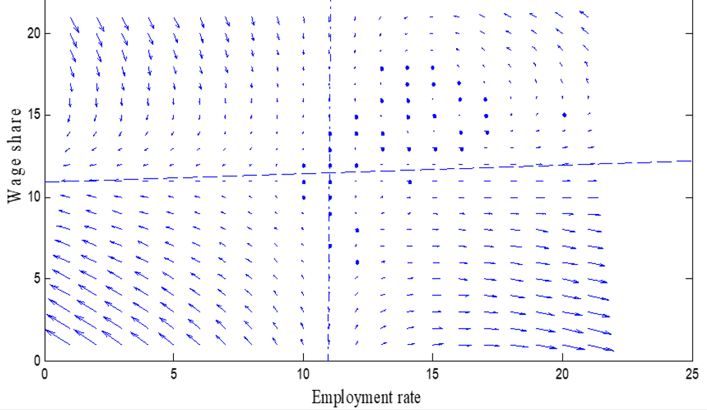
Juxtaposing this vector field (Figure 2) to the studies by [23, 27], and [19], around the origin \(\left(0,0\right)\) which happens to be the trivial solution to Model (4), the arrows are drifting away. It is most likely to be a saddle point. On the economic front, it is obvious that no economy will be willing to experience the situation where both employment rate and wage share go to zero simultaneously. Besides, a cursory look into the first quadrant of the vector field reveals that the arrows are circumnavigating around some given point. In the first quadrant, both employment rate and wage share take on positive values. Relating the field to the result in the quantitative analysis, it can suspected that the point around which the arrows are surrounding is the other equilibrium and desired solution, which might be a stable centre. This region becomes economically relevant, that is the first quadrant \(\left\{x>0,\ \ and\ y>0\right\}\) where both employment rate and wage share are positive.
Further qualitative analysis of Model (4) as indicated by [21] and [22] produced a periodic system typical of predator prey models. Figure 3 depicts the symbiotic relationship that exist between employment rate and wage share for the economy of Ghana between the period 1990 and 2008 inclusive.

From Figure 3, it is observed that both employment rate and wage share do not reach their maximum and minimum points at the same time whiles confirming Dawed’s [28] analogy that the carrying capacity of either variable sufficiently controls the type and stability of the predator-prey interaction. As corroborated in Becker and Leopold-Wildburger’s [4] study, for initial employment rate higher than initial wage share, this study show that employment rate reaches a maximum as wage share approximates zero. Successive periods in Figure 3 indicate that the maximum point achieved by wage share is higher than employment rate. More so, both employment rate and wage share are asymptotic to zero (as observed in the vector field analysis). Thus, no matter the rates of employment and wage share, neither variables will die out, nor will it grow infinitely. Figure 3 further show that employment rate drives wage share as employment rate move along its growth path. When initial employment rate is set lower than wage share, employment rate and wage share together begin by falling until a minimum is reached and then a growing trajectory. At peak levels, Figure 3 show that the maximum point reached by wage share is higher than employment rate. Again, where the initial value of wage share is set low, its trajectories in this case take a ‘U’ shape from the start.
Economically, at low remuneration, labour is reluctant to seek for employment so that capitalist desire to get high productivity from workers coupled with workers bargaining power, their remuneration increases. This increase in remuneration entices labour to seek for employment and the employment rate rises with the wage share since owners of capital now spend more on payment. As employment increases, workers voice weakens and capitalist are unwilling to increase the remuneration of workers because they must make profit, save to plough back into their business. Subsequently, retrenchment occurs, employment rate falls to a minimum till wages start to rise to entice some labour to join the working group. This interaction between employment rate and wage share in the economy according to literature [5, 16] would continue to exhibit such periodic state.
Liking to Becker and Leopold-Wildburger’s [4] illustrations, Figure 4 establishes the phase portrait of the solution and the stability of the Model (4), which represents the nonlinear interaction between employment rate and wage share returns on capital investment regime in Ghana for the period 1990 to 2008.

Changing initial values from (0.945, 0.0665462) to (0.97, 0.1417853) and to (0.953, 0.1370997), the result did not change. The phase portrait continued to exhibit stable and counter clockwise ellipses around the equilibrium solution \((0.84214756\mathrm{\ },0.976376199)\). This confirms that the equilibrium point\((0.84214756\mathrm{\ },0.976376199)\) is a stable centre. Therefore, for any given quantity \((x\left(0\right),y\left(0\right))\) with \(x(0)\neq 0\) and \(y(0)\neq 0\), other than the equilibrium \((0.84214756\mathrm{\ },0.976376199)\), the rates of employment and wage will oscillate cyclically.
As espoused by Becker and Leopold-Wildburger [4], for any initial conditions starting (other than (0, 0), the interdependence between employment rate and wage share will maintain a balance periodically with each varying between maximum and minimum values. Taking any of the solution curves, in the lower right quadrant, employment rate is increasing from a little below 0.1 to about 2.5 gently as wage share remains relatively constant a little above 0.0. However, between 2.5 and 3.9 where employment rate reaches its peak, employment rate increases precipitously as wage share also depicts a rise to a little below 1.0. In the upper right quadrant, after employment rate has achieved its peak of about 3.9, it starts to fall moderately until a little below 1.0. All things being equal, wage share now rises from a little below 1.0 to a maximum of about 4.0. In this climate, employment rate is reduced so that owners of capital can continue to increase the wage of the few in employment. As wage share increases however, capitalist are unable to save more of their profit to plough back in business suspending expansion. In the upper left corner of the phase portrait we observe that both employment rate and labour share are falling steadily. Whereas employment rate is falling from a about 1.0 to about 0.0, wage share is reducing from a little above 4.0 to a little below 1.0. Specifically, employment rate undergoes a sharp decline between 0.8 and 0.0 and maintains relatively a constant decline. Wage share also undergoes such a drastic reduction between the peak and 2.5 and then maintains a constant fall from 2.5 to about 0.9. For the lower left corner of Figure 4, both employment rate and wage share fall initially and then rise slowly. Both variables approach 0.0, but never get there.
Economically, in the lower left corner, both employment rate and wage share are so low that no economy would like to operate in this region. This is because once employment rate is low then only few people get employed leaving a huge unemployed labour. Again, because wage share is low, then this may reflect in low disposable income leading to low standard of living. In the upper left corner, since both employment rate and labour share are falling simultaneously to zero, it would not be a good region to operate. This analysis has confirmed the literature [4, 23] that the origin is an unwarranted point of operation in an economic discussion.
On the question of how long it takes for a cycle to traverse (go through a complete session), it was computed using the formula \(T=\frac{2\pi }{\sqrt{n_1n_2}}\), where \(n_1=\frac{1}{v}-\left(\propto +\beta \right)\) and \(n_2=\gamma +\propto\). By the values obtained under the simulation, \(n_1=4.88180995\), \(n_2=4.32692168\) and \(\pi ={22}/{7}\) thereby \(T=1.36764910\). This suggests that each cycle has a time length of about one year four months.
Data on the economic variables necessary for this project basically, labour force, unemployment rate, GDP, gross capital formation and the daily minimum wage figures were collected for this project. A predator-prey model was formulated and empirically tested using employment rate and the wage share returns on capital investment data. The model was robust for descriptive and predictive purposes. The model effectively captured the cyclical nature of the relationship between employment rates and wage shares, providing valuable insights into their mutual interactions. Mathematically, assumptions underpinning non-linear predator-prey models for example, population oscillation through time, and generating stable coexistence were met. Economically, wage share was driven by the employment rate further developing wave-like trajectories. More so, a basic principle in economics was established in that no matter the rates of employment and wage share, neither variables will die out, nor will it grow indefinitely. Arguably, there is an optimum achievable rate of stability.
This study modelled the interaction of only two production variables of wage share and employment rate in the broader real output economy. Given that the non-linear predation model was mathematically formulated and successively simulated, it is recommended in line with Grasselli and Maheshwari [23] that future studies should expand the number of economic variables to generate a more robust model comparable to exiting econometric models.
The model assumed a simplistic exponential growth rate of labour productivity although the graph of labour productivity compared well to a fourth-degree polynomial when plotted with MATLAB rather than the exponential growth model. Moreso, the data for the simulation is relatively old and spans on a short period, which may not represent current economic indicators.
Nevertheless, the use of exponential growth rates for predator and prey variables are widely used in literature hence, the results can be valid. Besides, it must be noted that the data is relevant not only for economic analysis, but for modelling differential equations. Despite the Model’s simplicity and limitations in this study, the results suggest that the simulated model can serve as a foundation for more complex models in studying endogenous growth cycles.
width=
| YearnGDP (GH m) | GDP Deflator | \(Q\) | K % GDP | K | \(v={K}/{Q}\) | w (GH ) | \(wL\) | P (`000) | N (`000) | L (`000) | \(a={Q}/{L}\) |
Modelled Labour
force |
Modelled Labour
productivity |
L% | Q% | K% | \(x={L}/{N}\) | \(y=wL/Q\) |
| 1990216 | 12.208 | 1769.33 | 14.44 | 255.49 | 0.1444 | 0.0218 | 117.742 | 14967.51 | 5715.363 | 5401.018 | 0.047304 | 5715.636 | 0.027197 | 0.945 | 0.0665462 | |||
| 1991270 | 14.527 | 1858.61 | 15.88 | 295.15 | 0.1588 | 0.046 | 263.524 | 15401.29 | 5905.954 | 5728.774 | 0.0515206 | 5905.954 | 0.041140305 | 6.1 | 5.0 | 15.5 | 0.97 | 0.1417853 |
| 1992295 | 15.102 | 1953.38 | 12.8 | 250.03 | 0.1280 | 0.046 | 267.803 | 15852.83 | 6108.915 | 5821.796 | 0.0429472 | 6102.901 | 0.05215544 | 1.6 | 5.1 | -15.3 | 0.953 | 0.137097 |
| 1993387 | 18.937 | 2043.62 | 22.21 | 453.89 | 0.2221 | 0.046 | 281.154 | 16316.16 | 6346.884 | 6112.049 | 0.0742615 | 6306.415 | 0.060619235 | 5.0 | 4.6 | 81.5 | 0.963 | 0.1375766 |
| 1994520 | 24.647 | 2109.79 | 23.96 | 505.51 | 0.2396 | 0.079 | 493.768 | 16782.49 | 6593.065 | 6250.226 | 0.0808787 | 6516.716 | 0.06690852 | 2.3 | 3.2 | 11.4 | 0.948 | 0.2340365 |
| 1995775 | 35.288 | 2196.21 | 20.02 | 439.89 | 0.2003 | 0.12 | 782.611 | 17245.46 | 6843.401 | 6521.761 | 0.0674496 | 6734.030 | 0.071400125 | 4.3 | 4.1 | -13.0 | 0.953 | 0.3563463 |
| 19961135 | 49.348 | 2299.99 | 21.2 | 487.6 | 0.2120 | 0.17 | 1140.92 | 17702.99 | 7079.421 | 6711.291 | 0.0726537 | 6958.590 | 0.07447088 | 2.9 | 4.7 | 10.8 | 0.948 | 0.4960541 |
| 19971411 | 58.949 | 2393.59 | 24.81 | 593.85 | 0.2481 | 0.2 | 1394.783 | 18154.03 | 7356.448 | 6973.913 | 0.0851531 | 7190.639 | 0.076497615 | 3.9 | 4.1 | 21.8 | 0.948 | 0.5827157 |
| 19981730 | 69.005 | 2507.06 | 23.11 | 579.38 | 0.2311 | 0.2 | 1467.666 | 18610.17 | 7620.280 | 7338.330 | 0.0789526 | 7430.426 | 0.07785716 | 5.2 | 4.7 | -2.4 | 0.963 | 0.5854132 |
| 19992058 | 78.625 | 2617.49 | 21 | 549.67 | 0.2100 | 0.29 | 2057.187 | 19066.60 | 7890.709 | 7093.747 | 0.0774865 | 7678.210 | 0.078926345 | -3.3 | 4.4 | -5.1 | 0.899 | 0.7859387 |
| 20002715 | 100 | 2715 | 24 | 651.6 | 0.24 | 0.42 | 3074.108 | 19529.31 | 8168.868 | 7319.306 | 0.0890248 | 7934.256 | 0.080082 | 3.2 | 3.7 | 18.5 | 0.896 | 1.1322683 |
| 20013807 | 134.580 | 2828.8 | 26.6 | 752.46 | 0.2660 | 0.55 | 4385.517 | 19999.19 | 8411.041 | 7973.667 | 0.0943681 | 8198.840 | 0.081700955 | 8.9 | 4.2 | 15.5 | 0.948 | 1.5503099 |
| 20024886 | 165.213 | 2957.39 | 19.7 | 582.61 | 0.1970 | 0.715 | 5898.411 | 20474.92 | 8656.376 | 8249.526 | 0.0706234 | 8472.249 | 0.08416004 | 3.5 | 4.5 | -22.6 | 0.953 | 1.9944652 |
| 20036616 | 212.542 | 3112.8 | 22.94 | 714.08 | 0.2294 | 0.92 | 7748.845 | 20954.56 | 8903.443 | 8422.657 | 0.0847808 | 8754.774 | 0.087836085 | 2.1 | 5.3 | 22.6 | 0.956 | 2.4893487 |
| 20047989 | 243.077 | 3286.61 | 28.38 | 932.74 | 0.2838 | 1.12 | 9717.186 | 21435.26 | 9151.961 | 8676.059 | 0.1075073 | 9046.721 | 0.09310592 | 3.0 | 5.6 | 30.6 | 0.948 | 2.9565985 |
| 20059726 | 279.540 | 3479.29 | 29 | 1008.99 | 0.2900 | 1.35 | 12400.071 | 21915.17 | 9401.472 | 9185.238 | 0.1098491 | 9348.403 | 0.100346375 | 5.9 | 5.9 | 8.2 | 0.977 | 3.56399661 |
| 200611672 | 315.209 | 3702.94 | 30.42 | 1126.43 | 0.3042 | 1.5 | 13636.963 | 22393.34 | 9651.071 | 9091.309 | 0.1239019 | 9660.145 | 0.10993428 | -1.0 | 6.4 | 11.6 | 0.942 | 3.6827395 |
| 200714046 | 358.953 | 3913.05 | 33.82 | 1323.39 | 0.3382 | 1.912 | 17950.912 | 22870.97 | 9903.536 | 9388.552 | 0.1409578 | 9982.284 | 0.122246465 | 3.3 | 5.7 | 17.5 | 0.948 | 4.5874476 |
| 200817618 | 419.770 | 4197.77 | 35.94 | 1508.68 | 0.3594 | 2.25 | 22033.498 | 23350.93 | 10158.367 | 9792.666 | 0.1540622 | 10315.164 | 0.13765976 | 4.3 | 7.3 | 14.0 | 0.964 | 5.2488579 |
| Av.4624.8 | 137.1 | 2733.8 | 23.7 | 684.8 | 0.2 | 0.6 | 5532.2 | 19106.5 | 7887.7 | 2733.8 | 0.1 | 3.4 | 4.9 | 12.3 | 0.9 | 1.6 | ||
|
Trading Economics (2010) http://www.tradingeconomics.com/ghana; Bank of Ghana http://www.bog.gov.gh; ILO Labour Statistics Database, (2010) http://www.laborsta.ilo.org/STP/guest; Ghana Statistical Service http://www.statsghana.gov.gh
Nominal GDP = nGDP; Real GDP = Q; Gross Capital Formation = K; Capital Output Ratio = v; Daily Minimum Wage = w; Wage Bill = wL; Total Population = P; Labour Force = N; Employed Labour = L; Labour Productivity = \(\alpha\)); Growth Rate of Employment = L%; Growth Rate of real GDP; Gross capital growth rate = K%; Employment level = x; Wage Share =y \(Employment=labour\ force\ -\ unemployment\ rate\times labour\ force\); \(Real\ GDP\ =\frac{nominal\ GDP\times GDP\ deflator}{100}\ at\ 2000\ base\ year\); \(Gross\ Capital\ Formation=gross\ capital\ formation\ rate\ per\ cent\times real\ GDP\); \(Wage\ bill=minimum\ wage\times number\ of\ employed\ labour\) The unemployment rate Ghana Living Standard Surveys (GLSS) of Ghana Statistical Service Nominal and Real GDP, and gross capital formation rates sourced from Trading Economics and the budget statements of various years. Daily minimum wage figures assessed from the Bank of Ghana website |
||||||||||||||||||