
In mathematics, the Riemann-Stieltjes integral (RS-integral) is a generalization of the Riemann integral. Following [1], the RS-integral is written in the form \(\int_{a}^{b}f\left( t\right) du(t)\), where the functions \(f\) and \(u\) are referred to as the integrand and the integrator, respectively. The RS-integral is used in several different areas of mathematics and its applications. These include reliability theory, statistics, the approximation of integral operators arising in electrical engineering, and the modelling of populations in mathematical biology, among other fields.
Numerical integration is one of the most well-studied areas in numerical analysis. The term quadrature is used to describe numerical integration in one dimension. Quadrature rules are widely used to approximate the RS-integral. Recent mathematical research has placed considerable emphasis on the problem of approximating the RS-integral, and several error bounds for the resulting approximations have been studied. Some of the most useful approximation formulas have been developed using Ostrowski-type and generalized trapezoid-type quadrature rules. Dragomir [2] considered the error associated with the following Ostrowski-type quadrature rule: \[\Theta \left( f,u;a,b,x\right) :=\int_{a}^{b}f\left( t\right) du\left( t\right) -f\left( x\right) \left[ u\left( b\right) -u\left( a\right) \right].\]
For various error bounds on the functional \(\Theta (f,u;a,b,x)\) under different assumptions on \(f\) and \(u\) for which the RS-integral exists, the reader may refer to [3–9] and the references therein.
From a different point of view, the authors of [10] considered the following generalized trapezoid rule: \[T\left( f,u;a,b,x\right) :=\int_{a}^{b}f\left( t\right) du\left( t\right) – \left[ u\left( b\right) -u\left( x\right) \right] f\left( b\right) -\left[ u\left( x\right) -u\left( a\right) \right] f\left( a\right) .\]
Several studies have investigated the problem of approximating the RS-integral using the generalized trapezoid rule under different assumptions on the functions \(f\) and \(u\) that ensure the existence of the RS-integral. For further results on these approximation formulas and their associated error bounds, the reader may refer to [5,8,10–14] and the references cited therein.
In [15], Alomari established the following companion of Ostrowski’s inequality for the RS-integral, where \(f\) is assumed to be of \(r\)–\(H\)–Hölder type and \(u\) is a monotonically nondecreasing function.
Theorem 1. Let \(f\) \(:\left[ a,b\right] \rightarrow \mathbb{R}\) be an \(r\)–\(H\)– Hölder type mapping, namely \[\left\vert f\left( t\right) -f\left( s\right) \right\vert \leq H\left\vert t-s\right\vert ^{r},\text{ for all }t,s\in \left[ a,b\right] ,\] where \(H>0\) and \(r\in \left( 0,1\right]\) are given and \(u\) \(:\left[ a,b\right] \rightarrow \mathbb{R}\) is a monotonically nondecreasing function on \(\left[ a,b\right]\). Then we have the inequality \[\begin{aligned} & \Big|\left[ u\left( \frac{a+b}{2}\right) -u\left( a\right) \right] f\left( x\right) +\left[ u(b)-u\left( \frac{a+b}{2}\right) \right] f\left( a+b-x\right) -\int_{a}^{b}f\left( t\right) du\left( t\right) \Big| \\ &\qquad \leq 2H\left[ \frac{b-a}{4}+\left\vert x-\frac{3a+b}{4}\right\vert \right] ^{r}\left[ u\left( \frac{a+b}{2}\right) -\frac{u(a)+u(b)}{2}\right], \end{aligned}\] for all \(x \in [a,\frac{a+b}{2}].\)
For other results concerning the companion of Ostrowski’s inequality, see [16–19]. In a recent contribution to the approximation of the RS-integral, the authors of [20] studied a three-point quadrature rule for integrands that are Lipschitzian or of bounded variation and for integrators that are of \(r\)–\(H\)-Hölder type. Motivated by the above results, in this paper we propose a new approach to approximate the RS-integral \(\int_{a}^{b}f\left( t\right) du(t)\) by the use of a four-point rule. More precisely, we establish bounds for the associated error functional \[\begin{aligned} G\left( f,u;a,b,x,\lambda \right):=&\left[ u\left( \frac{a+b}{2}\right) -\left( \left( 1-\lambda \right) u(x)+\lambda u(a\right) )\right] f\left( x\right) +\left( 1-\lambda \right) \left[ u(x)-u\left( a\right) \right] f\left( a\right) \\ & +\left[ \left( 1-\lambda \right) u(a+b-x)+\lambda u(b)-u\left( \frac{a+b}{2} \right) \right] f\left( a+b-x\right) \\ & +\left( 1-\lambda \right) \left[ u\left( b\right) -u\left( a+b-x\right) \right] f\left( b\right) -\int_{a}^{b}f\left( t\right) du\left( t\right), \end{aligned}\tag{1}\] where \(\lambda \in \left[ 0,1\right]\), \(x\in \left[ a,\frac{a+b}{2} \right]\) and we assume that the function \(f\) is Lipschitzian on \(\left[ a,b\right]\) and \(u\) is of \(r\)–\( H\)-Hölder type or bounded variation on \(\left[ a,b\right]\). The important case of weighted integrals is considered, composite quadrature rules are provided and applications to the approximation of Fourier transforms on finite intervals are also given.
Assume that \(u,\) \(f:\left[ a,b\right] \rightarrow \mathbb{C}\). If the RS-integral \(\int_{a}^{b}f\left( t\right) du\left( t\right)\) exists, we write for simplicity, following the notation in [1, p. 142], \(f\in \mathcal{R}_{\mathbb{C} }\left( u,\left[ a,b\right] \right) ,\) or \(\mathcal{R}_{_{\mathbb{C}}}\left( u\right)\) when the interval is implicitly known. If the functions \(u\) and \(f\) are real-valued, then we write \(f\in \mathcal{R}\left( u,\left[ a,b\right] \right) ,\) or \(\mathcal{R}\left( u\right) .\)
We start with the following identity of interest:
Lemma 1. Let \(f,\) \(u:\left[ a,b\right] \rightarrow \mathbb{C}\) be such that \(f\in \mathcal{R}_{\mathbb{C}}\left( u,\left[ a,b\right] \right)\). Then for any \(x\in \left[ a,\frac{a+b}{2}\right]\) and \(\gamma ,\) \(\mu \in \mathbb{C}\), \[\begin{aligned} & \left[ u\left( \frac{a+b}{2}\right) -\gamma \right] f\left( x\right) + \left[ \gamma -u\left( a\right) \right] f\left( a\right) +\left[ \mu -u\left( \frac{a+b}{2}\right) \right] f\left( a+b-x\right) + \left[ u\left( b\right) -\mu \right] f\left( b\right) -\int_{a}^{b}f\left( t\right) du\left( t\right) \\ &\qquad =\int_{a}^{x}\left[ u\left( t\right) -\gamma \right] df\left( t\right) +\int_{x}^{a+b-x}\left[ u\left( t\right) -u\left( \frac{a+b}{2}\right) \right] df\left( t\right) +\int_{a+b-x}^{b}\left[ u\left( t\right) -\mu \right] df\left( t\right) . \end{aligned}\tag{2}\]
Proof. Using the integration-by-parts rule for the RS-integral, we have \[\begin{aligned} \int_{a}^{x}\left[ u\left( t\right) -\gamma \right] df\left( t\right) =\left[ u\left( x\right) -\gamma \right] f\left( x\right) -\left[ u\left( a\right) -\gamma \right] f\left( a\right) -\int_{a}^{x}f\left( t\right) du\left( t\right), \end{aligned}\] and \[\begin{aligned} \int_{x}^{a+b-x}\left[ u\left( t\right) -u\left( \frac{a+b}{2}\right) \right] df\left( t\right) =&\left[ u\left( a+b-x\right) -u\left( \frac{a+b}{2}\right) \right] f\left( a+b-x\right) -\left[ u\left( x\right) -u\left( \frac{a+b}{2}\right) \right] f\left( x\right) \\ & -\int_{x}^{a+b-x}f\left( t\right) du\left( t\right), \end{aligned}\] and \[\begin{aligned} &\int_{a+b-x}^{b}\left[ u\left( t\right) -\mu \right] df\left( t\right) = \left[ u\left( b\right) -\mu \right] f\left( b\right) -\left[ u\left( a+b-x\right) -\mu \right] f\left( a+b-x\right)-\int_{a+b-x}^{b}f\left( t\right) du\left( t\right). \end{aligned}\]
If we add these three equalities, we get \[\begin{aligned} \int_{a}^{x}&\left[ u\left( t\right) -\gamma \right] df\left( t\right) +\int_{x}^{a+b-x}\left[ u\left( t\right) -u\left( \frac{a+b}{2}\right) \right] df\left( t\right) +\int_{a+b-x}^{b}\left[ u\left( t\right) -\mu \right] df\left( t\right) \\ =&\left[ u\left( x\right) -\gamma \right] f\left( x\right) -\left[ u\left( a\right) -\gamma \right] f\left( a\right) +\left[ u\left( a+b-x\right) -u\left( \frac{a+b}{2}\right) \right] f\left( a+b-x\right) \\ & -\left[ u\left( x\right) -u\left( \frac{a+b}{2}\right) \right] f\left( x\right) +\left[ u\left( b\right) -\mu \right] f\left( b\right) -\left[ u\left( a+b-x\right) -\mu \right] f\left( a+b-x\right) \\ & -\int_{a}^{x}f\left( t\right) du\left( t\right) -\int_{x}^{a+b-x}f\left( t\right) du\left( t\right) -\int_{a+b-x}^{b}f\left( t\right) du\left( t\right) \\ =&\left[ u\left( \frac{a+b}{2}\right) -\gamma \right] f\left( x\right) + \left[ \gamma -u\left( a\right) \right] f\left( a\right) +\left[ \mu -u\left( \frac{a+b}{2}\right) \right] f\left( a+b-x\right) \\ & +\left[ u\left( b\right) -\mu \right] f\left( b\right) -\int_{a}^{b}f\left( t\right) du\left( t\right), \end{aligned}\] for any \(x\in \left[ a,\frac{a+b}{2}\right]\), which proves the desired equality (2). \(\square\)
The following corollaries are of interest and will be used in the sequel.
Corollary 1. Let \(f,\) \(u:\left[ a,b\right] \rightarrow \mathbb{C}\) be such that \(f\in \mathcal{R}_{\mathbb{C}}\left( u,\left[ a,b\right] \right)\). Then for any \(\lambda \in \left[ 0,1\right]\) and \(x\in \left[ a,\frac{a+b}{2} \right]\) we have the representation \[\begin{aligned} G\left( f,u;a,b,x,\lambda \right) =&\int_{a}^{x}\left[ u\left( t\right) -\left( \left( 1-\lambda \right) u(x)\right) +\lambda u(a))\right] df\left( t\right) +\int_{x}^{a+b-x}\left[ u\left( t\right) -u\left( \frac{a+b}{2}\right) \right] df\left( t\right) \\ & +\int_{a+b-x}^{b}\left[ u\left( t\right) -\left( \left( 1-\lambda \right) u(a+b-x)+\lambda u(b)\right) \right] df\left( t\right), \end{aligned}\tag{3}\] where \(G\left( f,u;a,b,x,\lambda \right)\) is defined in (1).
The proof follows from (2) for \(\gamma =\left( 1-\lambda \right) u(x)+\lambda u(a),\) and \(\mu =\left( 1-\lambda \right) u(a+b-x)+\lambda u(b)\) and for any \(\lambda \in \left[ 0,1\right]\).
For \(\lambda =0\), we have \[\begin{aligned} G\left( f,u;a,b,x,0\right) :=&\left[ u\left( \frac{a+b}{2}\right) -u\left( x\right) \right] f\left( x\right) +\left[ u(x)-u\left( a\right) \right] f\left( a\right) \\ & +\left[ u(a+b-x)-u\left( \frac{a+b}{2}\right) \right] f\left( a+b-x\right)\\& + \left[ u\left( b\right) -u\left( a+b-x\right) \right] f\left( b\right) -\int_{a}^{b}f\left( t\right) du\left( t\right) \\ =&\int_{a}^{x}\left[ u\left( t\right) -u(x)\right] df\left( t\right) +\int_{x}^{a+b-x}\left[ u\left( t\right) -u\left( \frac{a+b}{2}\right) \right] df\left( t\right) \\ & +\int_{a+b-x}^{b}\left[ u\left( t\right) -u\left( a+b-x\right) \right] df\left( t\right) . \end{aligned}\]
For \(\lambda =1\), we have \[\begin{aligned} G\left( f,u;a,b,x,1\right) :=&\left[ u\left( \frac{a+b}{2}\right) -u\left( a\right) \right] f\left( x\right) +\left[ u(b) -u\left( \frac{a+b}{2}\right) \right] f\left( a+b-x\right) -\int_{a}^{b}f\left( t\right) du\left( t\right) \\ =&\int_{a}^{x}\left[ u\left( t\right) -u(a)\right] df\left( t\right) +\int_{x}^{a+b-x}\left[ u\left( t\right) -u\left( \frac{a+b}{2}\right) \right] df\left( t\right) \\ & +\int_{a+b-x}^{b}\left[ u\left( t\right) -u\left( b\right) \right] df\left( t\right) . \end{aligned}\]
For \(x=a\), we obtain \[\begin{aligned} G\left( f,u;a,b,a,\lambda \right) :=& \left[ u\left( \frac{a+b}{2}\right) -u\left( a\right) \right] f\left( a\right) +\left[ u(b)-u\left( \frac{a+b}{2}\right) \right] f\left( b\right) -\int_{a}^{b}f\left( t\right) du\left( t\right) \\ =& \int_{a}^{b}\left[ u\left( t\right) -u\left( \frac{a+b}{2}\right) \right] df\left( t\right). \end{aligned}\]
Corollary 2. Let \(f,\) \(u:\left[ a,b\right] \rightarrow \mathbb{C}\) be such that \(f\in \mathcal{R}_{\mathbb{C}}\left( u,\left[ a,b\right] \right)\). Then for any \(\lambda \in \left[ 0,1\right]\) \[\begin{aligned} G\left( f,u;a,b,\frac{3a+b}{4},\lambda \right) :=& \left[ u\left( \frac{a+b}{2}\right) -\left( (1-\lambda )u\left( \frac{3a+b}{4}\right) +\lambda u\left( a\right) \right)\right] f\left( \frac{3a+b}{4}\right) \\ &+ (1-\lambda )\left[ u\left( \frac{3a+b}{4}\right) -u\left( a\right) \right] f\left( a\right)\\ &+\left[ (1-\lambda )u\left( \frac{a+3b}{4}\right) +\lambda u\left( b\right) -u\left( \frac{a+b}{2}\right) \right] f\left( \frac{a+3b}{4}\right) \\ & +(1-\lambda )\left[ u(b)-u\left( \frac{a+3b}{4}\right) \right] f\left( b\right) -\int_{a}^{b}f\left( t\right) du\left( t\right) \\ =&\int_{a}^{\frac{3a+b}{4}}\left[ u\left( t\right) -\left((1-\lambda )u\left( \frac{3a+b}{4}\right) +\lambda u(a)\right)\right] df\left( t\right) \\ &+ \int_{\frac{3a+b}{4}}^{\frac{a+3b}{4}}\left[ u\left( t\right) -u\left(\frac{a+b}{2}\right)\right] df\left( t\right) \\ & +\int_{\frac{a+3b}{4}}^{b}\left[ u\left( t\right) -\left((1-\lambda )u\left( \frac{a+3b}{4}\right) +\lambda u\left( b\right) \right)\right] df\left( t\right) . \end{aligned}\tag{4}\]
The proof follows from Corollary 1 for \(x=\frac{3a+b}{4}.\)
For \(\lambda =1/2,\) we obtain \[\begin{aligned} G\left( f,u;a,b,\frac{3a+b}{4},1/2\right) :=&\left[ u\left( \frac{a+b}{2}\right) -\frac{1}{2}\left( u\left( \frac{3a+b}{4}\right) + u\left( a\right)\right )\right] f\left( \frac{3a+b}{4}\right) \\ &+ \frac{1}{2}\left[ u\left( \frac{3a+b}{4}\right) -u\left( a\right) \right] f\left( a\right)\\ &+\left[ \frac{1}{2}\left(u\left( \frac{a+3b}{4}\right) + u\left( b\right)\right) -u\left( \frac{a+b}{2}\right) \right] f\left( \frac{a+3b}{4}\right) \\ & +\frac{1}{2}\left[ u(b)-u\left( \frac{a+3b}{4}\right) \right] f\left( b\right) -\int_{a}^{b}f\left( t\right) du\left( t\right) \\ =&\int_{a}^{\frac{3a+b}{4}}\left[ u\left( t\right) -\frac{1}{2}\left( u\left( \frac{3a+b}{4}\right) + u\left( a\right)\right )\right] df\left( t\right) \\ &+ \int_{\frac{3a+b}{4}}^{\frac{a+3b}{4}}\left[ u\left( t\right) -u\left(\frac{a+b}{2}\right)\right] df\left( t\right) \\ & +\int_{\frac{a+3b}{4}}^{b}\left[ u\left( t\right)-\frac{1}{2}\left( u\left( \frac{a+3b}{4}\right) + u\left( b\right)\right )\right] df\left( t\right) . \end{aligned}\tag{5}\]
If \(u\) is an integral, namely \(u (t) := \int _a^ t w (s) ds\), where \(w\) is integrable on \(\left[ a,b\right]\), then we can state the following identity as well:
Corollary 3. Assume that \(w\) is integrable on \(\left[ a,b\right]\) and let \(f\) be a function of bounded variation on \(\left[ a,b\right]\) such that \(wf\) is also integrable on \( \left[ a,b\right]\). Then we have the equality \[\begin{aligned} G \left( f,\int_{a}^{\cdot }w\left( s\right) ds;a,b,x,\lambda \right) :=&f\left( x\right)\left[\lambda\int_{a}^{x}w\left( s\right) ds+\int_{x}^{\frac{a+b}{2}}w\left( s\right) ds\right]+f\left( a\right)\left[ (1-\lambda)\int_{a}^{ x}w\left( s\right) ds \right] \\ & +f\left( a+b-x\right) \left[\int_{\frac{a+b}{2}}^{a+b-x}w\left( s\right) ds +\lambda \int_{a+b-x}^{b} w\left( s\right) ds\right] \\ &+ f\left( b\right) \left[ (1-\lambda)\int_{a+b- x}^{b}w\left( s\right) ds\right]-\int_{a}^{b}f\left( s\right) w\left( s\right) ds \\ =&\int_{a}^{x}\left[\lambda \int_{a}^{t}w\left(s\right) ds -( 1-\lambda)\int_{t}^{x}w\left(s\right) ds \right] df\left( t\right) \\ &+\int_{x}^{a+b-x}\left[ \int_{\frac{a+b}{2}}^{t}w\left(s\right) ds \right] df\left( t\right) \\ &+ \int_{a+b-x}^{b} \bigg[(1-\lambda)\int_{a+b-x}^{t}w\left(s\right) ds-\lambda \int_{t}^{b}w\left(s\right) ds\bigg] df\left( t\right) , \end{aligned}\tag{6}\] where \(\lambda \in \left[ 0,1\right]\) and \(x \in (a,\frac{a+b}{2}).\)
If we take \(\lambda =1/2 , x= \frac{3a+b}{4}\), then we obtain \[\begin{aligned} G \left( f,\int_{a}^{\cdot }w\left( s\right) ds;a,b,\frac{3a+b}{4},1/2 \right) :=&f\left( \frac{3a+b}{4}\right)\left[\frac{1}{2}\int_{a}^{\frac{3a+b}{4}}w\left( s\right) ds+\int_{\frac{3a+b}{4}}^{\frac{a+b}{2}}w\left( s\right) ds\right]+f\left( a\right)\left[ \frac{1}{2}\int_{a}^{ \frac{3a+b}{4}}w\left( s\right) ds \right] \\ & +f\left( \frac{a+3b}{4}\right) \left[\int_{\frac{a+b}{2}}^{\frac{a+3b}{4}}w\left( s\right) ds +\frac{1}{2} \int_{\frac{a+3b}{4}}^{b} w\left( s\right) ds\right] \\ &+ f\left( b\right) \left[ \frac{1}{2}\int_{\frac{a+3b}{4}}^{b}w\left( s\right) ds\right]-\int_{a}^{b}f\left( s\right) w\left( s\right) ds \\ =&\frac{1}{2}\int_{a}^{\frac{3a+b}{4}}\left[\int_{a}^{t}w\left(s\right) ds- \int_{t}^{\frac{3a+b}{4}}w\left(s\right) ds \right] df\left( t\right)+\int_{\frac{3a+b}{4}}^{\frac{a+3b}{4}}\left[ \int_{\frac{a+b}{2}}^{t}w\left(s\right) ds \right] df\left( t\right) \\ &+\frac{1}{2} \int_{\frac{a+3b}{4}}^{b} \bigg[\int_{\frac{a+3b}{4}}^{t}w\left(s\right) ds-\int_{t}^{b}w\left(s\right) ds\bigg] df\left( t\right) . \end{aligned}\]
The following theorem provides upper error bounds for the functional \(G\left( f,u;a,b,x,\lambda \right)\) in the case when \(f\) is Lipschitzian with the constant \(L>0,\) and \(u\) is an \(r\)–\(H\)-Hölder-type mapping with the constant \(H\) and exponent \(r\in \left( 0,1\right]\).
Theorem 2. Let \(f,\) \(u:\left[ a,b\right] \rightarrow \mathbb{C}\) and \( x\in \left[ a,\frac{a+b}{2}\right]\). If \(f\) is Lipschitzian with the constant \(L>0,\) namely \[\left\vert f\left( t\right) -f\left( s\right) \right\vert \leq L\left\vert t-s\right\vert, \text{ for all }t,\text{ }s\in \left[ a,b\right],\] and \(u\) is of \(r\)–\(H\)-Hölder type with the constant \(H\) and \(r\in \left( 0,1\right] ,\) namely \[\left\vert u\left( t\right) -u\left( s\right) \right\vert \leq H\left\vert t-s\right\vert ^{r},\text{ for all }t,\text{ }s\in \left[ a,b\right] ,\] then \(f\in \mathcal{R}_{\mathbb{C}}\left( u,\left[ a,b\right] \right)\) and we have the inequality:
\[\begin{aligned} \left\vert G(f,u;a,b,x,\lambda )\right\vert \leq & \frac{2LH}{r+1} \times \Bigg[(x-a)^{r+1}+\left( \frac{a+b}{2} -x\right) ^{r+1} \Bigg], \end{aligned}\tag{7}\] for \(\lambda \in \left[ 0,1\right]\).
Proof. It is well known that, if \(p:\left[ a,b\right] \rightarrow \mathbb{C}\) is Riemann integrable and \(v:\left[ a,b\right] \rightarrow \mathbb{C}\) is Lipschitzian with the constant \(L>0\), then the RS-integral \( \int_{a}^{b}p\left( t\right) dv\left( t\right)\) exists and the following inequality holds: \[\left\vert \int_{a}^{b}p\left( t\right) dv\left( t\right) \right\vert \leq L\int_{a}^{b}\left\vert p\left( t\right) \right\vert dt.\]
From the identity (3) and the properties of the integral, we then have \[\begin{aligned} \left\vert G(f,u;a,b,x,\lambda )\right\vert =&\left\vert \int_{a}^{x}\Big[u(t)-\big((1-\lambda )u(x)+\lambda u(a)\big) \Big]\,df(t)\right. +\int_{x}^{a+b-x}\Big[u(t)-u\!\left( \tfrac{a+b}{2}\right) \Big]\,df(t) \\ & \left. +\int_{a+b-x}^{b}\Big[u(t)-\big((1-\lambda )u(a+b-x)+\lambda u(b)\big) \Big]\,df(t)\right\vert \\ \leq& \left\vert \int_{a}^{x}\Big[u(t)-\big((1-\lambda )u(x)+\lambda u(a) \big)\Big]\,df(t)\right\vert +\left\vert \int_{x}^{a+b-x}\Big[u(t)-u\!\left( \tfrac{a+b}{2}\right) \Big] \,df(t)\right\vert \\ & +\left\vert \int_{a+b-x}^{b}\Big[u(t)-\big((1-\lambda )u(a+b-x)+\lambda u(b) \big)\Big]\,df(t)\right\vert \\ \leq& L\int_{a}^{x}\left\vert u(t)-((1-\lambda )u(x)+\lambda u(a))\right\vert dt +L\int_{x}^{a+b-x}\left\vert u(t)-u\!\left( \tfrac{a+b}{2}\right) \right\vert dt \\ & +L\int_{a+b-x}^{b}\left\vert u(t)-((1-\lambda )u(a+b-x)+\lambda u(b))\right\vert dt, \end{aligned}\tag{8}\] for \(\lambda \in \left[ 0,1\right]\) and \(x \in \left[ a,\frac{a+b}{2} \right]\).
Since \(u\) is of \(r\)–\(H\)-Hölder type with the constant \(H\), we have \[\begin{aligned} \int_{a}^{x}\Big|u(t)-\big((1-\lambda )u(x)+\lambda u(a)\big)\Big|\,dt \leq& (1-\lambda )\int_{a}^{x}|u(t)-u(x)|\,dt+\lambda \int_{a}^{x}|u(t)-u(a)|\,dt \\ \leq& H\left[ (1-\lambda )\int_{a}^{x}|t-x|^{r}\,dt+\lambda \int_{a}^{x}|t-a|^{r}\,dt\right] \\ =&\frac{H}{r+1}\left[ (1-\lambda )(x-a)^{r+1}+\lambda (x-a)^{r+1}\right] \\ =&\frac{H}{r+1}(x-a)^{r+1}. \end{aligned}\]
Observe that \[\begin{aligned} \int_{x}^{a+b-x}\left\vert u(t)-u\!\left( \tfrac{a+b}{2}\right) \right\vert dt \leq & H\int_{x}^{a+b-x}\left\vert t-\frac{a+b}{2}\right\vert ^{r}dt \\= & \frac{2H}{r+1}\left( \frac{a+b}{2}-x\right) ^{r+1}. \end{aligned}\] and \[\begin{aligned} & \int_{a+b-x}^{b}\left\vert u(t)-((1-\lambda )u(a+b-x)+\lambda u(b))\right\vert dt \\ \leq & (1-\lambda )\int_{a+b-x}^{b}\left\vert u(t)-u(a+b-x)\right\vert dt+\lambda \int_{a+b-x}^{b}\left\vert u(t)-u(b)\right\vert dt \\ \leq & H\left[ (1-\lambda )\int_{a+b-x}^{b}\left\vert t-(a+b-x)\right\vert ^{r}dt+\lambda \int_{a+b-x}^{b}\left\vert t-b\right\vert ^{r}dt\right] \\ = & \frac{H}{r+1}\left[ (1-\lambda ) (x-a)^{r+1} +\lambda (x-a)^{r+1}\right]\\ = & \frac{H}{r+1}(x-a)^{r+1}. \end{aligned}\]
By making use of (8) we obtain the error bound from (7). \(\square\)
Corollary 4. Assume that \(f\) and \(u\) satisfy the hypotheses of Theorem 2. We consider the following two choices:
1) For \(x=a\), we obtain \[|G\left( f,u;a,b,a,\lambda \right) |\leq \frac{2LH}{r+1}\left( \frac{b-a}{2} \right) ^{r+1}.\]
2) For \(x=\frac{3a+b}{4}\), we obtain \[\left\vert G(f,u;a,b,\frac{3a+b}{4},\lambda )\right\vert \leq \frac{4LH}{r+1} \left( \frac{b-a}{4}\right) ^{r+1}.\]
The case when \(u\) is the integral of another function is important for applications since it provides weighted integral rules in which the weight function can serve as the kernel of an integral transform, such as the Laplace, Fourier, or Mellin transform.
We recall Hölder’s integral inequality \[\left\vert \int_{c}^{d}h\left( t\right) g\left( t\right) dt\right\vert \leq \left( \int_{c}^{d}\left\vert h\left( t\right) \right\vert ^{\alpha }dt\right) ^{1/\alpha }\left( \int_{c}^{d}\left\vert g\left( t\right) \right\vert ^{\beta }dt\right) ^{1/\beta }, \tag{9}\] where \(\alpha ,\beta >1\) with \(\frac{1}{\alpha }+\frac{1}{\beta }=1\) and the integrals on the right side are finite.
If we take \(u\left( t\right) =\int_{a}^{t}w\left( \tau \right) d\tau\) and use (9), then we get \[\begin{aligned} \left\vert u\left( t\right) -u\left( s\right) \right\vert = & \left\vert \int_{a}^{t}w\left( \tau \right) d\tau -\int_{a}^{s}w\left( \tau \right) d\tau \right\vert =\left\vert \int_{s}^{t}w\left( \tau \right) d\tau \right\vert \\ \leq & \left\vert \int_{s}^{t}1d\tau \right\vert ^{^{1/\alpha }}\left\vert \int_{s}^{t}\left\vert w\left( \tau \right) \right\vert ^{\beta }d\tau \right\vert ^{1/\beta }=\left\vert t-s\right\vert ^{^{1/\alpha }}\left\vert \int_{s}^{t}\left\vert w\left( \tau \right) \right\vert ^{\beta }d\tau \right\vert ^{1/\beta } \\ \leq & \left\vert t-s\right\vert ^{^{1/\alpha }}\left( \int_{a}^{b}\left\vert w\left( \tau \right) \right\vert ^{\beta }d\tau \right) ^{1/\beta }, \end{aligned}\] for all \(t,s\in \left[ a,b\right] .\)
This shows that the function \(u\left( t\right) =\int_{a}^{t}w\left( \tau \right) d\tau\) is of \(r\)–\(H\)-Hölder type with the exponent \(r=\frac{1 }{\alpha }<1\) and the positive constant \(H=\left( \int_{a}^{b}\left\vert w\left( \tau \right) \right\vert ^{\beta }d\tau \right) ^{1/\beta },\) provided that this integral is finite.
Corollary 5. By making use of the inequality (7) for \( u\left( t\right) =\int_{a}^{t}w\left( \tau \right) d\tau ,\) \(r=\frac{1}{ \alpha }<1\) and \(H=\left( \int_{a}^{b}\left\vert w\left( \tau \right) \right\vert ^{\beta }d\tau \right) ^{1/\beta },\) where \(\alpha ,\beta >1\) with \(\frac{1}{\alpha }+\frac{1}{\beta }=1\), \[\begin{aligned} \left\vert G(f,\int_{a}^{\cdot }w\left( s\right) ds;a,b,x,\lambda )\right\vert \leq \frac{2L\alpha}{\alpha+1} \left( \int_{a}^{b}\left\vert w\left( \tau \right) \right\vert ^{\beta }d\tau \right) ^{1/\beta } \times \Bigg[ (x-a)^{\frac{\alpha+1}{\alpha}}+\left( \frac{a+b}{2} -x\right) ^{\frac{\alpha+1}{\alpha}} \Bigg], \end{aligned}\tag{10}\] for \(x \in [a,\frac{a+b}{2}].\)
If \(x=\frac{3a+b}{4}\) we obtain the following weighted inequalities \[\begin{aligned} \left\vert G \left( f,\int_{a}^{\cdot }w\left( s\right) ds;a,b,\frac{3a+b}{4},\lambda \right) \right\vert \leq \frac{4L\alpha }{\alpha +1}\left( \int_{a}^{b}\left\vert w\left( \tau \right) \right\vert ^{\beta }d\tau \right) ^{1/\beta } \left( \frac{b-a}{4}\right) ^{\frac{\alpha+1}{\alpha}}. \end{aligned}\]
The following theorem provides upper error bounds in the case when \(f\) is Lipschitzian with the constant \( L>0,\) and \(u\) is of bounded variation.
Theorem 3. Let \(f,u\) \(:\left[ a,b\right] \rightarrow \mathbb{C}\) and \(x\in \left[ a,\frac{a+b}{2}\right]\). If \(f\) is Lipschitzian with the constant \( L>0,\) namely \[\left\vert f\left( t\right) -f\left( s\right) \right\vert \leq L\left\vert t-s\right\vert, \text{ for all }t,\text{ }s\in \left[ a,b\right],\] and \(u\) is of bounded variation, then we have the inequality \[\begin{aligned} |G\left( f,u;a,b,x,\lambda \right) | \leq L\max \bigg\{ \max \{\lambda ,1-\lambda \}(x-a),(a+b-2x)\bigg\} \bigvee\limits_{a}^{b}\left( u\right) . \end{aligned}\tag{11}\]
Proof. It is well known that, if \(p:\left[ a,b\right] \rightarrow \mathbb{C}\) is Riemann integrable and \(v:\left[ a,b\right] \rightarrow \mathbb{C}\) is Lipschitzian with the constant \(L>0\), then the RS-integral \( \int_{a}^{b}p\left( t\right) dv\left( t\right)\) exists and the following inequality holds: \[\left\vert \int_{a}^{b}p\left( t\right) dv\left( t\right) \right\vert \leq L\int_{a}^{b}\left\vert p\left( t\right) \right\vert dt.\] From the identity (3) and the properties of the integral, we then have \[\begin{aligned} \left\vert G(f,u;a,b,x,\lambda )\right\vert = & \left\vert \int_{a}^{x}\Big[u(t)-\big((1-\lambda )u(x)+\lambda u(a)\big) \Big]\,df(t)\right. +\int_{x}^{a+b-x}\Big[u(t)-u\!\left( \tfrac{a+b}{2}\right) \Big]\,df(t) \\ & \left. +\int_{a+b-x}^{b}\Big[u(t)-\big((1-\lambda )u(a+b-x)+\lambda u(b)\big) \Big]\,df(t)\right\vert \\ \leq & \left\vert \int_{a}^{x}\Big[u(t)-\big((1-\lambda )u(x)+\lambda u(a) \big)\Big]\,df(t)\right\vert +\left\vert \int_{x}^{a+b-x}\Big[u(t)-u\!\left( \tfrac{a+b}{2}\right) \Big] \,df(t)\right\vert \\ & +\left\vert \int_{a+b-x}^{b}\Big[u(t)-\big((1-\lambda )u(a+b-x)+\lambda u(b) \big)\Big]\,df(t)\right\vert \\ \leq & L\int_{a}^{x}\left\vert u(t)-((1-\lambda )u(x)+\lambda u(a))\right\vert dt +L\int_{x}^{a+b-x}\big\vert u(t)-u\!\left( \tfrac{a+b}{2}\right) \big\vert dt \\ & +L\int_{a+b-x}^{b}\left\vert u(t)-((1-\lambda )u(a+b-x)+\lambda u(b))\right\vert dt \\ = & :A(f,u;a,b,x,\lambda ), \end{aligned}\tag{12}\] for \(\lambda \in \left[ 0,1\right]\) and \(x\in \left[ a,\frac{a+b}{2} \right]\).
Since \(u\) is of bounded variation, we can state that \[\begin{aligned} \Big\vert (u(t)-(1-\lambda )u(x)-\lambda u(a)\Big\vert = & \Big\vert [\lambda (u(t)-u(a))+(1-\lambda )(u(t)-u(x))]\Big\vert \ \\ \leq & \lambda \Big\vert u(t)-u(a)\Big\vert +(1-\lambda )\Big\vert u(x)-u(t)\Big\vert \ \\ \leq & \lambda \bigvee\limits_{a}^{t}\left( u\right) +(1-\lambda )\bigvee\limits_{t}^{x}\left( u\right) \leq \max \left\{ \lambda ,1-\lambda \right\} \bigvee\limits_{a}^{x}\left( u\right) . \end{aligned}\]
Observe that \[\begin{aligned} &\left\vert u(t)-u\left( \frac{a+b}{2}\right) \right\vert \leq \bigvee\limits_{x}^{a+b-x}\left( u\right), \end{aligned}\] and \[\begin{aligned} \Big\vert (u(t)-(1-\lambda )u(a+b-x)-\lambda u(b)\Big\vert = & \Big\vert [(1-\lambda )(u(t)-u(a+b-x))+\lambda (u(t)-u(b))]\Big\vert \\ \leq & (1-\lambda )\Big\vert u(t)-u(a+b-x)\Big\vert +\lambda \Big\vert u(b)-u(t)\Big\vert \ \\ \leq & (1-\lambda )\bigvee\limits_{a+b-x}^{t}\left( u\right) +\lambda \bigvee\limits_{t}^{b}\left( u\right) \leq \max \left\{ \lambda ,1-\lambda \right\} \bigvee\limits_{a+b-x}^{b}\left( u\right), \end{aligned}\] for \(\lambda \in \left[ 0,1\right]\) and \(x\in \left[ a,\frac{a+b}{2}\right]\).
If we add these three inequalities, we derive
\[\begin{aligned}
A(f,u;a,b,x,\lambda )\leq& L\max \left\{ \lambda ,1-\lambda \right\}
\bigvee\limits_{a}^{x}\left( u\right)
\int_{a}^{x}dt +L\bigvee\limits_{x}^{a+b-x}\left( u\right) \int_{x}^{a+b-x}dt
+L\max \left\{ \lambda ,1-\lambda \right\} \bigvee\limits_{a+b-x}^{b}\left(
u\right) \int_{a+b-x}^{b}dt \\
= & L\max \left\{ \lambda ,1-\lambda \right\} \left( x-a\right)
\bigvee\limits_{a}^{x}\left( u\right) +L\left( a+b-2x\right)
\bigvee\limits_{x}^{a+b-x}\left( u\right) \\
& +L \max \left\{ \lambda ,1-\lambda \right\} \bigvee\limits_{a+b-x}^{b}\left(
u\right) \left( x-a\right) \\
\leq & L\max \bigg\{ \max \{\lambda ,1-\lambda \}(x-a),(a+b-2x)\bigg\}
\bigvee\limits_{a}^{b}\left( u\right),
\end{aligned}\] for \(\lambda \in \left[ 0,1\right]\) and \(x\in \left[ a,\frac{a+b}{2}\right]\).
The theorem is thus proved. \(\square\)
Corollary 6. Let \(f,\) \(u:\left[ a,b\right] \rightarrow \mathbb{C}\) be as in Theorem 3. Assume that \(\lambda \in \left[ 0,1\right]\). In (11), consider the following two choices:
1) For \(x=a\), we obtain \[|G\left( f,u;a,b,a,\lambda \right) |\leq L (b-a)\bigvee\limits_{a}^{b}\left( u\right) . \]
2) For \(x=\frac{3a+b}{4}\), we obtain \[\begin{aligned} |G\left( f,u;a,b,\frac{3a+b}{4},\lambda \right) | \leq & L\max \bigg\{ \max \{\lambda ,1-\lambda \}\left(\frac{b-a}{4}\right),\left(\frac{b-a}{2}\right)\bigg\} \bigvee\limits_{a}^{b}\left( u\right) . \end{aligned}\]
Corollary 7. By making use of the inequality (11) for \( u\left( t\right) =\int_{a}^{t}w\left( \tau \right) d\tau\) we obtain \[\begin{aligned} \left\vert G \left( f,\int_{a}^{\cdot }w\left( s\right) ds;a,b,x,\lambda \right)\right\vert \leq & L \max\Big\{ \max \{\lambda ,1-\lambda \}(x-a),(a+b-2x)\Big\} \int_a^b |w(s)| ds, \end{aligned}\tag{13}\] for \(x \in [a,\frac{a+b}{2}].\)
If \(\lambda=1/2\) and \(x=\frac{3a+b}{4}\) we obtain the following weighted inequalities \[\begin{aligned} \left\vert G \left( f,\int_{a}^{\cdot }w\left( s\right) ds;a,b,\frac{3a+b}{4},1/2 \right) \right\vert \leq L\max \bigg\{ \frac{1}{2}\left(\frac{b-a}{4}\right),\left(\frac{b-a}{2}\right)\bigg\} \int_a^b |w(s)| ds . \end{aligned}\]
Let \(I_{n}:a=x_{0}<x_{1}<…<x_{n-1}<x_{n}=b\) be a partition of the interval \( \left[ a,b\right]\). Set \(h_{k}:=x_{k+1}-x_{k}\quad (k=0,\dots ,n-1)\) and \( \nu (h):=\max \{h_{k}|k=0,…,n-1\}\) and choose an intermediate point vector \( \mathcal{\xi }=(\xi _{0},\xi _{1},\dots ,\xi _{n-1})\) such that \(\xi _{k}\in \left[ x_{k},\frac{{x_k}+x_{k+1}}{2}\right]\) for \(k=0,1,\dots ,n-1\), where \(\lambda \in \left[ 0,1\right]\). Define the sum associated with the partition \( I_{n}\) and the intermediate points \(\mathcal{\xi }\) by \[\begin{aligned} \Psi \left( f,I_{n},\mathcal{\xi },\lambda \right) :=&\sum_{k=0}^{n-1}f\left( \xi_{k}\right) \left[\lambda\int_{x_{k}}^{\xi_{k}}w\left( s\right) ds+\int_{\xi_{k}}^{\frac{x_{k}+x_{k+1}}{2}}w\left( s\right) ds\right]+\sum_{k=0}^{n-1}f\left( x_{k}\right)\left[ (1-\lambda)\int_{x_{k}}^{ \xi_{k}}w\left( s\right) ds \right] \\ & +\sum_{k=0}^{n-1}f\left( x_{k}+x_{k+1}-\xi_{k}\right) \left[ \int_{\frac{x_k+x_{k+1}}{2}}^{x_k+x_{k+1}-\xi_k}w\left( s\right) ds +\lambda \int_{x_k+x_{k+1}-\xi_{k}}^{x_{k+1}} w\left( s\right) ds\right] \\ &+ \sum_{k=0}^{n-1}f\left( x_{k+1}\right) \left[ (1-\lambda)\int_{ x_x+x_{k+1}-\xi_{k}}^{x_{k+1}}w\left( s\right) ds\right], \end{aligned}\tag{14}\] and the error of approximation for the weighted integral \( \int_{a}^{b}f\left( s\right) w\left( s\right) ds\) by \(\Psi \left( f,I_{n}, \mathcal{\xi },\lambda \right) ,\) namely \[\mathcal{R}\left( f,I_{n},\mathcal{\xi },\lambda \right) :=\Psi \left( f,I_{n},\mathcal{\xi },\lambda \right) -\int_{a}^{b}f\left( s\right) w\left( s\right) ds. \tag{15}\]
The following result provides an error bound in the case when \(f\) is Lipschitzian with the constant \(L>0\) and the weight \(w\) satisfies the condition that the integral \(\int_{a}^{b}\left\vert w\left( \tau \right) \right\vert ^{\beta }d\tau\) is finite.
Theorem 4. Assume that \(f\) is Lipschitzian with the constant \(L>0\) and the weight \(w\) is such that the integral \(\int_{a}^{b}\left\vert w\left( \tau \right) \right\vert ^{\beta }d\tau\) is finite, where \(\alpha ,\beta >1\) with \(\frac{1}{ \alpha }+\frac{1}{\beta }=1\). Let \(I_{n}\) be a partition of \(\left[ a,b\right]\) and let the intermediate point vector be \(\mathcal{\xi }=(\xi _{0},\xi _{1},\dots ,\xi _{n-1}).\) Then for \(\lambda \in \left[ 0,1\right]\) we have the error bounds \[\begin{aligned} \left\vert \mathcal{R}\left( f,I_{n},\mathcal{\xi },\lambda \right) \right\vert \leq & \frac{2L\alpha}{\alpha+1} \left( \int_{a}^{b}\left\vert w\left( \tau \right) \right\vert ^{\beta }d\tau \right) ^{1/\beta } \frac{\nu(h)}{2}\times \bigg[\left( \sum_{k=0}^{n-1}\left( \xi _{k}-x_{k}\right) \right) ^{1/\alpha }+\left( \sum_{k=0}^{n-1}\left( \frac{x_{k}+x_{k+1}}{2}-\xi_k\right) \right) ^{1/\alpha }\bigg]\\ \leq & \frac{2L\alpha}{\alpha+1} \left( \int_{a}^{b}\left\vert w\left( \tau \right) \right\vert ^{\beta }d\tau \right) ^{1/\beta } \left( \frac{b-a}{2}\right) ^{1/\alpha }{\nu(h)}. \end{aligned}\tag{16}\]
Proof. By making use of the inequality (10) written for the interval \(
\left[ x_{k},x_{k+1}\right]\) and the intermediate point \(\xi _{k}\in
\left[ x_{k},\frac{{x_k}+x_{k+1}}{2}\right]\) for \(k=0,1,\dots ,n-1\) we have
\[\begin{aligned}
& \Bigg\vert f\left( \xi_k\right)\left[\lambda\int_{x_k}^{\xi_k}w\left(
s\right) ds+\int_{\xi_k}^{\frac{x_k+x_{k+1}}{2}}w\left(
s\right) ds\right]+f\left( x_k\right) (1-\lambda)\int_{x_k}^{
\xi_k}w\left( s\right) ds \\
& +f\left( x_k+x_{k+1}-\xi_k\right) \left[ \int_{\frac{x_k+x_{k+1}}{2}}^{x_k+x_{k+1}-\xi_k}w\left( s\right) ds +\lambda \int_{x_k+x_{k+1}-\xi_k}^{x_{k+1}}w\left( s\right) ds\right] \\
&+ f\left( x_{k+1}\right) (1-\lambda)\int_{ x_k+x_{k+1}-\xi_k}^{x_{k+1}}w\left(
s\right) ds-\int_{x_k}^{x_{k+1}}f\left( s\right) w\left(
s\right) ds \Bigg \vert \\
&\qquad \leq \frac{2L\alpha}{\alpha+1} \left( \int_{x_k}^{x_{k+1}}\left\vert w\left( \tau
\right) \right\vert ^{\beta }d\tau \right) ^{1/\beta } \times \Bigg[(\xi_{k}-x_k)^{\frac{\alpha+1}{\alpha}}+\left( \frac{x_k+x_{k+1}}{2}
-\xi_{k}\right) ^{\frac{\alpha+1}{\alpha}} \Bigg],
\end{aligned}\] for \(k=0,1,\dots ,n-1\), which by summation gives \[\begin{aligned}
& \sum_{k=0}^{n-1} \Bigg\vert f\left( \xi_k\right)\left[\lambda\int_{x_k}^{\xi_k}w\left(
s\right) ds+\int_{\xi_k}^{\frac{x_k+x_{k+1}}{2}}w\left(
s\right) ds\right]+f\left( x_k\right) (1-\lambda)\int_{x_k}^{
\xi_k}w\left( s\right) ds \\
& +f\left( x_k+x_{k+1}-\xi_k\right) \left[ \int_{\frac{x_k+x_{k+1}}{2}}^{x_k+x_{k+1}-\xi_k}w\left( s\right) ds +\lambda \int_{x_k+x_{k+1}-\xi_k}^{x_{k+1}} w\left( s\right) ds\right] \\
&+ f\left( x_{k+1}\right) (1-\lambda)\int_{ x_k+x_{k+1}-\xi_k}^{x_{k+1}}w\left(
s\right) ds-\int_{x_k}^{x_{k+1}}f\left( s\right) w\left(
s\right) ds \Bigg \vert \\
&\qquad \leq \frac{2L\alpha}{\alpha+1} \sum_{k=0}^{n-1}\left( \int_{x_k}^{x_{k+1}}\left\vert w\left( \tau
\right) \right\vert ^{\beta }d\tau \right) ^{1/\beta } \times \Bigg[(\xi_{k}-x_k)^{\frac{\alpha+1}{\alpha}}+\left( \frac{x_k+x_{k+1}}{2}
-\xi_{k}\right) ^{\frac{\alpha+1}{\alpha}} \Bigg].
\end{aligned}\]
By the generalized triangle inequality for the modulus, we have \[\begin{aligned} & \sum_{k=0}^{n-1} \left\vert f\left( \xi_k\right)\Bigg[\lambda\int_{x_k}^{\xi_k}w\left( s\right) ds+\int_{\xi_k}^{\frac{x_k+x_{k+1}}{2}}w\left( s\right) ds\right]+f\left( x_k\right)(1-\lambda)\int_{x_k}^{ \xi_k}w\left( s\right) ds \\ & +f\left( x_k+x_{k+1}-\xi_k\right) \left[ \int_{\frac{x_k+x_{k+1}}{2}}^{x_k+x_{k+1}-\xi_k}w\left( s\right) ds +\lambda \int_{x_k+x_{k+1}-\xi_k}^{x_{k+1}} w\left( s\right) ds\right] \\ &+ f\left( x_{k+1}\right) (1-\lambda)\int_{ x_k+x_{k+1}-\xi_k}^{x_{k+1}}w\left( s\right) ds-\int_{x_k}^{x_{k+1}}f\left( s\right) w\left( s\right) ds \Bigg\vert \\ &\quad \geq \left\vert \sum_{k=0}^{n-1}f\left( \xi_k\right)\Bigg[\lambda\int_{x_k}^{\xi_k}w\left( s\right) ds +\int_{\xi_k}^{\frac{x_k+x_{k+1}}{2}}w\left( s\right) ds\right]+ \sum_{k=0}^{n-1}f\left( x_k\right)\left[ (1-\lambda)\int_{x_k}^{ \xi_k}w\left( s\right) ds \right] \\ & \qquad+ \sum_{k=0}^{n-1} f\left( x_k+x_{k+1}-\xi_k\right) \left[\int_{\frac{x_k+x_{k+1}}{2}}^{x_k+x_{k+1}-\xi_k}w\left( s\right) ds +\lambda \int_{x_k+x_{k+1}-\xi_k}^{x_{k+1}} w\left( s\right) ds\right] \\ &\qquad+ \sum_{k=0}^{n-1}f\left( x_{k+1}\right) \left[ (1-\lambda)\int_{ x_k+x_{k+1}-\xi_k}^{x_{k+1}}w\left( s\right) ds\Bigg] -\sum_{k=0}^{n-1}\int_{x_{k}}^{x_{k+1}}f\left( s\right) w\left( s\right) ds\right\vert \\ &\quad= \left\vert \Psi \left( f,I_{n},t,\lambda \right) -\int_{a}^{b}f\left( s\right) w\left( s\right) ds\right\vert , \end{aligned}\tag{17}\] and \[\begin{aligned} &\sum_{k=0}^{n-1}\left( \int_{x_k}^{x_{k+1}}\left\vert w\left( \tau \right) \right\vert ^{\beta }d\tau \right) ^{1/\beta } \times \Bigg[(\xi_{k}-x_k)^{\frac{\alpha+1}{\alpha}}+\left( \frac{x_k+x_{k+1}}{2} -\xi_{k}\right) ^{\frac{\alpha+1}{\alpha}} \Bigg] \\ & =\sum_{k=0}^{n-1}\left( \int_{x_k}^{x_{k+1}}\left\vert w\left( \tau \right) \right\vert ^{\beta }d\tau \right) ^{1/\beta } (\xi_{k}-x_k)^{\frac{\alpha+1}{\alpha}} +\sum_{k=0}^{n-1}\left( \int_{x_k}^{x_{k+1}}\left\vert w\left( \tau \right) \right\vert ^{\beta }d\tau \right) ^{1/\beta } \left( \frac{x_k+x_{k+1}}{2} -\xi_{k}\right) ^{\frac{\alpha+1}{\alpha}} . \end{aligned}\]
By the discrete form of Hölder’s inequality for \(\alpha ,\beta >1\) with \(\frac{1}{\alpha }+\frac{1}{\beta }=1,\) namely \[\sum_{k=0}^{n-1}a_{i}b_{i}\leq \left( \sum_{k=0}^{n-1}a_{i}^{\beta }\right) ^{1/\beta }\left( \sum_{k=0}^{n-1}b_{i}^{\alpha }\right) ^{1/\alpha },\] we deduce that \[\begin{aligned} \sum_{k=0}^{n-1}\left( \int_{x_{k}}^{x_{k+1}}\left\vert w\left( \tau \right) \right\vert ^{\beta }d\tau \right) ^{1/\beta }\left( \xi _{k}-x_{k}\right) ^{\frac{\alpha +1}{\alpha }} \leq & \left( \sum_{k=0}^{n-1}\left[ \left( \int_{x_{k}}^{x_{k+1}}\left\vert w\left( \tau \right) \right\vert ^{\beta }d\tau \right) ^{1/\beta }\right] ^{\beta }\right) ^{1/\beta }\left( \sum_{k=0}^{n-1}\left[ \left( \xi _{k}-x_{k}\right) ^{\frac{\alpha +1}{\alpha }}\right] ^{\alpha }\right) ^{1/\alpha } \\ \leq & \left( \sum_{k=0}^{n-1}\int_{x_{k}}^{x_{k+1}}\left\vert w\left( \tau \right) \right\vert ^{\beta }d\tau \right) ^{1/\beta }\left( \sum_{k=0}^{n-1}\left( \xi _{k}-x_{k}\right) ^{\alpha +1}\right) ^{1/\alpha } \\ \leq & \left( \int_{a}^{b}\left\vert w\left( \tau \right) \right\vert ^{\beta }d\tau \right) ^{1/\beta }\left( \sum_{k=0}^{n-1}\left( \xi _{k}-x_{k}\right) ^{\alpha +1}\right) ^{1/\alpha }. \end{aligned}\]
We observe that \[\begin{aligned} \sum_{k=0}^{n-1}&\left( \int_{x_k}^{x_{k+1}}\left\vert w\left( \tau \right) \right\vert ^{\beta }d\tau \right) ^{1/\beta } \left( \frac{x_k+x_{k+1}}{2} -\xi_{k}\right) ^{\frac{\alpha+1}{\alpha}} \\ \leq & \left( \sum_{k=0}^{n-1}\left[ \left( \int_{x_{k}}^{x_{k+1}}\left\vert w\left( \tau \right) \right\vert ^{\beta }d\tau \right) ^{1/\beta }\right] ^{\beta }\right) ^{1/\beta }\left( \sum_{k=0}^{n-1}\left[ \left( \frac{x_k+x_{k+1}}{2} -\xi_{k}\right) ^{\frac{\alpha +1}{\alpha }}\right] ^{\alpha }\right) ^{1/\alpha } \\ \leq & \left( \sum_{k=0}^{n-1}\int_{x_{k}}^{x_{k+1}}\left\vert w\left( \tau \right) \right\vert ^{\beta }d\tau \right) ^{1/\beta }\left( \sum_{k=0}^{n-1}\left( \frac{x_k+x_{k+1}}{2} -\xi_{k}\right) ^{\alpha +1}\right) ^{1/\alpha }\\ \leq & \left( \int_{a}^{b}\left\vert w\left( \tau \right) \right\vert ^{\beta }d\tau \right) ^{1/\beta }\left( \sum_{k=0}^{n-1} \left( \frac{x_k+x_{k+1}}{2} -\xi_{k}\right) ^{\alpha +1}\right) ^{1/\alpha }.\\ \end{aligned}\] Also, observe that \[\begin{aligned} \left( \sum_{k=0}^{n-1}\left( \xi _{k}-x_{k}\right) ^{\alpha +1}\right) ^{1/\alpha }=& \left( \sum_{k=0}^{n-1}\left( \xi _{k}-x_{k}\right) ^{\alpha } \left( \xi _{k}-x_{k}\right)\right) ^{1/\alpha }\\ \leq & \frac{\nu(h)}{2} \left( \sum_{k=0}^{n-1}\left( \xi _{k}-x_{k}\right) \right) ^{1/\alpha } \\ \leq & \frac{\nu(h)}{2} \left( \sum_{k=0}^{n-1}\left( \frac{x_{k+1}-x_{k}}{2}\right) \right) ^{1/\alpha }=\frac{\nu(h)}{2} \left( \frac{b-a}{2}\right) ^{1/\alpha } \end{aligned}\] and \[\begin{aligned} \left( \sum_{k=0}^{n-1}\left( \frac{x_{k}+x_{k+1}}{2}-\xi _{k}\right) ^{\alpha +1}\right) ^{1/\alpha }=& \left( \sum_{k=0}^{n-1}\left( \frac{x_{k}+x_{k+1}}{2}-\xi _{k}\right) ^{\alpha }\left(\frac{x_{k}+x_{k+1}}{2}-\xi _{k}\right)\right) ^{1/\alpha }\\ \leq & \frac{\nu(h)}{2} \left( \sum_{k=0}^{n-1}\left( \frac{x_{k}+x_{k+1}}{2}-\xi_k\right) \right) ^{1/\alpha }\\ \leq & \frac{\nu(h)}{2} \left( \sum_{k=0}^{n-1}\left( \frac{x_{k+1}-x_{k}}{2}\right) \right) ^{1/\alpha } =\frac{\nu(h)}{2} \left( \frac{b-a}{2}\right) ^{1/\alpha }. \end{aligned}\]
Therefore \[\begin{aligned} \sum_{k=0}^{n-1}&\left( \int_{x_k}^{x_{k+1}}\left\vert w\left( \tau \right) \right\vert ^{\beta }d\tau \right) ^{1/\beta } (\xi_{k}-x_k)^{\frac{\alpha+1}{\alpha}}+\sum_{k=0}^{n-1}\left( \int_{x_k}^{x_{k+1}}\left\vert w\left( \tau \right) \right\vert ^{\beta }d\tau \right) ^{1/\beta } \left( \frac{x_k+x_{k+1}}{2} -\xi_{k}\right) ^{\frac{\alpha+1}{\alpha}} \\ \leq & \left( \int_{a}^{b}\left\vert w\left( \tau \right) \right\vert ^{\beta }d\tau \right) ^{1/\beta } \sum_{k=0}^{n-1} (\xi_{k}-x_k)^{\frac{\alpha+1}{\alpha}} +\left( \int_{a}^{b}\left\vert w\left( \tau \right) \right\vert ^{\beta }d\tau \right) ^{1/\beta } \sum_{k=0}^{n-1}\left( \frac{x_k+x_{k+1}}{2} -\xi_{k}\right) ^{\frac{\alpha+1}{\alpha}} \\ \leq & \left( \int_{a}^{b}\left\vert w\left( \tau \right) \right\vert ^{\beta }d\tau \right) ^{1/\beta } \frac{\nu(h)}{2} \left( \sum_{k=0}^{n-1}\left( \xi_{k}-x_{k}\right) \right) ^{1/\alpha } + \left( \int_{a}^{b}\left\vert w\left( \tau \right) \right\vert ^{\beta }d\tau \right) ^{1/\beta } \frac{\nu(h)}{2} \left( \sum_{k=0}^{n-1}\left( \frac{x_{k}+x_{k+1}}{2}-\xi_k\right) \right) ^{1/\alpha }\\ =& \left( \int_{a}^{b}\left\vert w\left( \tau \right) \right\vert ^{\beta }d\tau \right) ^{1/\beta } \frac{\nu(h)}{2} \times \bigg[\left( \sum_{k=0}^{n-1}\left( \xi_{k}-x_{k}\right) \right) ^{1/\alpha }+\left( \sum_{k=0}^{n-1}\left( \frac{x_{k}+x_{k+1}}{2}-\xi_k\right) \right) ^{1/\alpha }\bigg]\\ \leq & \left( \int_{a}^{b}\left\vert w\left( \tau \right) \right\vert ^{\beta }d\tau \right) ^{1/\beta } 2 \left( \frac{b-a}{2}\right) ^{1/\alpha }\frac{\nu(h)}{2} \\=& \left( \int_{a}^{b}\left\vert w\left( \tau \right) \right\vert ^{\beta }d\tau \right) ^{1/\beta } \left( \frac{b-a}{2}\right)^{1/\alpha } {\nu(h)}, \end{aligned}\] which completes the proof. \(\square\)
Remark 1. Assume that \(f\) is Lipschitzian with the constant \(L>0\) and the weight \(w\) is such that the integral \(\int_{a}^{b}\left\vert w\left( \tau \right) \right\vert ^{\beta }d\tau\) is finite, where \(\alpha ,\beta >1\) with \(\frac{1}{ \alpha }+\frac{1}{\beta }=1\). By taking the intermediate point vector \(\xi _{m}:=\left( \xi _{0},…,\xi _{n-1}\right) ,\) where \(\xi _{k}=\frac{ 3x_{k}+x_{k+1}}{4}\) for all \(k=0,1,\dots ,n-1\), we obtain the following identity for \(\lambda \in \left[ 0,1\right]\): \[\mathcal{R}_{1}\left( f,I_{n},\xi _{m},\lambda \right) :=\Psi _{1}\left( f,I_{n},\xi _{m},,\lambda \right) -\int_{a}^{b}f\left( s\right) w\left( s\right) ds,\] where \[\begin{aligned} \Psi _{1}\left( f,I_{n},\xi _{m},\lambda \right) :=&\sum_{k=0}^{n-1}f\left( \frac{3x_{k}+x_{k+1}}{4}\right) \left[ \lambda \int_{x_{k}}^{\frac{3x_{k}+x_{k+1}}{4}}w\left( s\right) ds+\int_{\frac{3x_{k}+x_{k+1}}{4}}^{ \frac{x_{k}+x_{k+1}}{2}}w\left( s\right) ds\right] \\ & +\sum_{k=0}^{n-1}f\left( x_{k}\right) \left[ (1-\lambda )\int_{x_{k}}^{ \frac{3x_{k}+x_{k+1}}{4}}w\left( s\right) ds\right] \\ & +\sum_{k=0}^{n-1}f\left( \frac{x_{k}+3x_{k+1}}{4}\right) \left[ \int_{ \frac{x_{k}+x_{k+1}}{2}}^{\frac{x_{k}+3x_{k+1}}{4}}w\left( s\right) ds+\lambda \int_{\frac{x_{k}+3x_{k+1}}{4}}^{x_{k+1}}w\left( s\right) ds \right] \\ & +\sum_{k=0}^{n-1}f\left( x_{k+1}\right) \left[ (1-\lambda )\int_{\frac{ x_{k}+3x_{k+1}}{4}}^{x_{k+1}}w\left( s\right) ds\right] , \end{aligned}\tag{18}\] and the remainder \(\left\vert \mathcal{R}_{1}\left( f,I_{n},\xi _{m},\lambda \right) \right\vert\) satisfies the bound \[\begin{aligned} \left\vert \mathcal{R}_{1}\left( f,I_{n},\xi _{m},\lambda \right) \right\vert \leq & \frac{2L\alpha }{(\alpha +1)}\left( \int_{a}^{b}\left\vert w\left( \tau \right) \right\vert ^{\beta }d\tau \right) ^{1/\beta }\frac{\nu (h)}{4} \times \left[\left( \sum_{k=0}^{n-1}\left( \xi _{k}-x_{k}\right) \right) ^{1/\alpha }+\left( \sum_{k=0}^{n-1}\left( \frac{x_{k}+x_{k+1}}{2}-\xi _{k}\right) \right) ^{1/\alpha }\right] \\ \leq & \frac{L\alpha }{(\alpha +1)}\left( \int_{a}^{b}\left\vert w\left( \tau \right) \right\vert ^{\beta }d\tau \right) ^{1/\beta }\left( \frac{b-a}{4}\right) ^{1/\alpha }{\nu (h)}. \end{aligned}\tag{19}\]
The case in which \(f\) is Lipschitzian and the weight is integrable is covered by the following result.
Theorem 5. Assume that \(f\) is Lipschitzian with the constant \(L>0\) and the weight \(w\) is such that the integral \(\int_{a}^{b}\left\vert w\left( \tau \right) \right\vert d\tau\) is finite. Let \(I_{n}\) be a partition of \(\left[ a,b\right]\) and let the intermediate point vector be \(\mathcal{\xi }=(\xi _{0},\xi _{1},\dots ,\xi _{n-1}).\) Then for \(\lambda \in \left[ 0,1\right]\) we have the error bound \[\begin{aligned} \left\vert \mathcal{R}\left( f,I_{n},\mathcal{\xi },\lambda \right) \right\vert \leq& L \max_{k=0,\dots,n-1} \bigg[ \max \left\{ \lambda ,1-\lambda \right\} \left( \xi_k-x_k\right) ,\left( x_k+x_{k+1}-2\xi_k\right)\bigg]\int_{a}^{b} |w(s) |ds\\ \leq & L \max_{k=0,\dots,n-1} \bigg[ \max \left\{ \lambda ,1-\lambda \right\} \frac{\nu(h)}{2},\nu(h)\bigg]\int_{a}^{b} |w(s)| ds. \end{aligned}\tag{20}\]
Proof. By making use of the inequality (13) written for the interval \( \left[ x_{k},x_{k+1}\right]\) and the intermediate points \(\xi _{k}\in \left[ x_{k},\frac{{x_k}+x_{k+1}}{2}\right]\) for \(k=0,1,\dots ,n-1\) we have \[\begin{aligned} & \Bigg\vert f\left( \xi_k\right)\left[\lambda\int_{x_k}^{\xi_k}w\left( s\right) ds+\int_{\xi_k}^{\frac{x_k+x_{k+1}}{2}}w\left( s\right) ds\right]+f\left( x_k\right) (1-\lambda)\int_{x_k}^{ \xi_k}w\left( s\right) ds \\ & +f\left( x_k+x_{k+1}-\xi_k\right) \left[ \int_{\frac{x_k+x_{k+1}}{2}}^{x_k+x_{k+1}-\xi_k}w\left( s\right) ds +\lambda \int_{x_k+x_{k+1}-\xi_k}^{x_{k+1}} w\left( s\right) ds\right] \\ &+ f\left( x_{k+1}\right) (1-\lambda)\int_{x_k+x_{k+1}- \xi_k}^{x_{k+1}}w\left( s\right) ds-\int_{x_k}^{x_{k+1}}f\left( s\right) w\left( s\right) ds \Bigg \vert \\ &\qquad\leq L \max \bigg[\max \left\{ \lambda ,1-\lambda \right\} \left( \xi_k-x_k\right) ,\left( x_k+x_{k+1}-2\xi_k\right) \bigg]\int_{x_k}^{x_{k+1}} |w(s)| ds, \end{aligned}\] for \(k=0,1,\dots ,n-1\), which by summation gives \[\begin{aligned} & \sum_{k=0}^{n-1} \Bigg\vert f\left( \xi_k\right)\left[\lambda\int_{x_k}^{\xi_k}w\left( s\right) ds+\int_{\xi_k}^{\frac{x_k+x_{k+1}}{2}}w\left( s\right) ds\right]+f\left( x_k\right) (1-\lambda)\int_{x_k}^{ \xi_k}w\left( s\right) ds \\ & +f\left( x_k+x_{k+1}-\xi_k\right) \left[\int_{\frac{x_k+x_{k+1}}{2}}^{x_k+x_{k+1}-\xi_k}w\left( s\right) ds +\lambda \int_{x_k+x_{k+1}-\xi_k}^{x_{k+1}} w\left( s\right) ds\right] \\ &+ f\left( x_{k+1}\right) (1-\lambda)\int_{ x_k+x_{k+1}-\xi_k}^{x_{k+1}}w\left( s\right) ds-\int_{x_k}^{x_{k+1}}f\left( s\right) w\left( s\right) ds \Bigg \vert \\ &\qquad\leq L \sum_{k=0}^{n-1} \max \bigg[ \max \left\{ \lambda ,1-\lambda \right\} \left( \xi_k-x_k\right) ,\left( x_k+x_{k+1}-2\xi_k\right)\bigg] \int_{x_k}^{x_{k+1}}| w(s) |ds\\ &\qquad\leq L \max_{k=0,\dots,n-1} \bigg[ \max \left\{ \lambda ,1-\lambda \right\} \left( \xi_k-x_k\right) ,\left( x_k+x_{k+1}-2\xi_k\right)\bigg]\sum_{k=0}^{n-1} \int_{x_k}^{x_{k+1}}| w(s)| ds \\ &\qquad\leq L \max_{k=0,\dots,n-1} \bigg[ \max \left\{ \lambda ,1-\lambda \right\} \left( \xi_k-x_k\right) ,\left( x_k+x_{k+1}-2\xi_k\right)\bigg]\int_{a}^{b} |w(s)| ds\\ &\qquad\leq L \max_{k=0,\dots,n-1} \bigg[ \max \left\{ \lambda ,1-\lambda \right\} \frac{\nu(h)}{2} ,\nu(h)\bigg]\int_{a}^{b} |w(s)| ds, \end{aligned}\] which completes the proof. \(\square\)
Remark 2. Assume that \(f\) is Lipschitzian with the constant \(L>0\) and the weight \(w\) is such that the integral \(\int_{a}^{b}\left\vert w\left( \tau \right) \right\vert d\tau\) is finite. For any value of the parameter \(\lambda \in \left[ 0,1\right]\), choose \(\xi _{k}=\frac{ 3x _{k}+x _{k+1}}{4}\) for all \(k=0,1,\dots ,n-1\). Then we have \[\mathcal{R}_2\left( f,I_{n},\lambda \right) :=\Psi_1 \left( f,I_{n},\lambda \right) -\int_{a}^{b}f\left( s\right) w\left( s\right) ds,\] where \(\Psi_1 \left( f,I_{n},\lambda \right)\) is given in (18) and the remainder \(\left\vert \mathcal{R}_2\left( f,I_{n},\lambda \right) \right\vert\) satisfies the bound \[\begin{aligned} \left\vert \mathcal{R}_2\left( f,I_{n},\lambda \right) \right\vert \leq & L \max_{k=0,\dots,n-1} \bigg[ \max \left\{ \lambda ,1-\lambda \right\} \frac{\nu(h)}{4} ,\frac{\nu(h)}{2}\bigg]\int_{a}^{b} |w(s)| ds\\=& L \frac{\nu(h)}{2}\int_{a}^{b}| w(s)| ds. \end{aligned}\]
The Fourier transform is one of the most essential tools of the mathematical sciences. It appears in unexpected applications in fields as diverse as differential equations, numerical analysis, probability theory, number theory, quantum mechanics, optics, medical imaging, and signal processing [21].
Let \(g:\left[ a,b\right] \rightarrow \mathbb{R}\) be a Lebesgue integrable mapping defined on the finite interval \(\left[ a,b\right]\) and let \(\mathcal{F} (g)\) denote its finite Fourier transform on the interval \(\left[ a,b\right]\), i.e. \[\mathcal{F}(g)(w):=\int_{a}^{b}g(s)e^{-2\pi iws}ds,\text{ }w\in \mathbb{R}.\]
The following inequality for the Fourier transform of functions of bounded variation was obtained in [22]:
Theorem 6. Let \(g:\left[ a,b\right] \rightarrow \mathbb{R}\) be a mapping of bounded variation on \(\left[ a,b\right]\). Then we have the inequality \[\left\vert \mathcal{F}(g)(w)-E(-2\pi iwa,-2\pi iwb)\int_{a}^{b}g(t)dt\right\vert \leq \frac{3}{4}\left( b-a\right) \bigvee_{a}^{b}\left( g\right),\] for all \(w\in \mathbb{R},\,w\neq 0\), where \(\bigvee\limits_{a}^{b} \left( g\right)\) is the total variation of \(g\) on \([a,b]\), and \(E\) denotes the exponential mean of two complex numbers, that is, \[E(z,w):= \begin{cases} \frac{e^{z}-e^{w}}{z-w} & \text{if }z\neq w, \\ & \\ exp(w) & \text{if }z=w, \end{cases} \quad ,z,\omega \in \mathbb{C}\text{.}\]
Now, for \(w(s)=e^{-2\pi its},\) \(t,s\in \mathbb{R}\) we have that \[\int_{c}^{d}e^{-2\pi its}ds=\left( d-c\right) E(-2\pi itc,-2\pi itd),\] for any real numbers \(c\), \(d\), and \(t\). Using this formula, we then have by (6) that \[\begin{aligned} G \left( f,\int_{a}^{\cdot }e^{-2\pi its}ds;a,b,x,\lambda \right) =& f\left( x\right)\left[\lambda\int_{a}^{x} e^{-2\pi its} ds+\int_{x}^{\frac{a+b}{2}}e^{-2\pi its} ds\right] +f\left( a\right) (1-\lambda)\int_{a}^{ x}e^{-2\pi its} ds \\ & +f\left( a+b-x\right) \left[ \int_{\frac{a+b}{2}}^{a+b-x}e^{-2\pi its} ds +\lambda\int_{a+b-x}^{b}e^{-2\pi its}ds\right] \\ &+ f\left( b\right) (1-\lambda)\int_{ a+b-x}^{b}e^{-2\pi its} ds -\int_{a}^{b}f\left( s\right)e^{-2\pi its}ds \qquad\qquad \mbox{which becomes}\\ = & f\left( x\right) \Bigg[\lambda\left(x-a\right)E(-2\pi itx,-2\pi ita)+ \left(\frac{a+b}{2}-x\right) \\ & \times E\left(-2\pi it\left(\frac{a+b}{2}\right) ,-2\pi itx\right)\Bigg] + f\left( a\right) (1-\lambda)\left(x-a\right) \\ & \times E(-2\pi itx,-2\pi ita) + f\left( a+b-x\right) \Bigg[\left((a+b-x)-\frac{a+b}{2}\right)\\ & \times E\left(-2\pi it(a+b-x),-2\pi it\left(\frac{a+b}{2}\right)\right)+\lambda \left(b-(a+b-x)\right) \\ & \times E\left(-2\pi itb ,-2\pi it\left(a+b-x\right)\right)\Bigg] + f\left( b\right) (1-\lambda)\left(b-(a+b-x)\right)\\ & \times E(-2\pi itb,-2\pi it(a+b-x))- \mathcal{F}(f)(t)\qquad\qquad\qquad\qquad \mbox{and}\\ =& f\left( x\right) \Bigg[\lambda\left(x-a\right)E(-2\pi itx,-2\pi ita)+ \left(\frac{a+b}{2}-x\right) \\& \times E\left(-2\pi it\left(\frac{a+b}{2}\right) ,-2\pi itx\right)\Bigg] + f\left( a\right) (1-\lambda)\left(x-a\right) \\ & \times E(-2\pi itx,-2\pi ita) + f\left( a+b-x\right) \Big[\left(\frac{a+b}{2}-x\right) \\ & \times E\left(-2\pi it(a+b-x),-2\pi it\left(\frac{a+b}{2}\right)\right)+\lambda \left(x-a\right) \\& \times E(-2\pi itb,-2\pi it\left(a+b-x\right) )\Big]+ f\left( b\right) (1-\lambda)\left(x-a\right) \\& \times E(-2\pi itb,-2\pi it(a+b-x))- \mathcal{F}(f)(t), \end{aligned}\] where \(\lambda \in \left[ 0,1\right],\ t \in \mathbb{R}, \,\ t\neq 0,\) and \(x\in [a,\frac{a+b}{2}].\)
Now, by making use of the inequality (10) for \(w(s)=e^{-2\pi
its},\) which gives \(\left( \int_{a}^{b}\left\vert w\left( \tau \right)
\right\vert ^{\beta}d\tau \right) ^{1/\beta}\\=\left( b-a\right) ^{1/\beta
},\) where \(\alpha,\beta>1\) with \(\frac{1}{\alpha }+\frac{1}{\beta}=1,\) we get the following error bound in approximating the Fourier transform in the case when \(f\) is a Lipschitzian function: \[\begin{aligned}
&\Bigg |f\left( x\right) \bigg[\lambda\left(x-a\right)E(-2\pi itx,-2\pi ita) + \left(\frac{a+b}{2}-x\right)\times E(-2\pi it\left(\frac{a+b}{2}\right) ,-2\pi itx)\bigg]+ f\left( a\right) (1-\lambda)\left(x-a\right)\\
& \times E(-2\pi itx,-2\pi ita) + f\left( a+b-x\right) \bigg[\left(\frac{a+b}{2}-x\right) \times E(-2\pi it(a+b-x),-2\pi it\left(\frac{a+b}{2}\right))+\lambda \left(x-a\right) \\ &\times E(-2\pi itb,-2\pi it\left(a+b-x\right) )\bigg]+ f\left( b\right) (1-\lambda)\left(x-a\right)\times E(-2\pi itb,-2\pi it(a+b-x))- \mathcal{F}(f)(t) \bigg|\\
&\qquad\leq \frac{2L\alpha }{\alpha +1}\left(b-a \right) ^{1/\beta } \left[\left(x-a\right)^{\frac{\alpha+1}{\alpha}} +\left(\frac{a+b}{2}-x\right)^{\frac{\alpha+1}{\alpha}} \right],
\end{aligned}\] for \(x\in [a,\frac{a+b}{2}],\) \(t \in \mathbb{R}, \, t\neq 0,\) and \(\lambda \in \left[ 0,1\right]\).
For \(\lambda=1/2\) we get \[\begin{aligned}
&\Bigg |f\left( x\right) \bigg[\frac{1}{2}\left(x-a\right)E(-2\pi itx,-2\pi ita)+ \left(\frac{a+b}{2}-x\right) \times E\left(-2\pi it\left(\frac{a+b}{2}\right) ,-2\pi itx\right)\bigg] + \frac{1}{2}f\left( a\right) \left(x-a\right) \\
& \times E(-2\pi itx,-2\pi ita) + f\left( a+b-x\right) \bigg[\left(\frac{a+b}{2}-x\right) \times E\left(-2\pi it(a+b-x),-2\pi it\left(\frac{a+b}{2}\right)\right)+\frac{1}{2}\left(x-a\right) \\
& \times E\left(-2\pi itb,-2\pi it\left(a+b-x\right) \right)\bigg] + \frac{1}{2}f\left( b\right) \left(x-a\right) \times E(-2\pi itb,-2\pi it(a+b-x))- \mathcal{F}(f)(t) \bigg|\\
&\qquad\leq \frac{2L\alpha }{(\alpha +1)}\left(b-a\right) ^{1/\beta } \left[\left(x-a\right)^{\frac{\alpha+1}{\alpha}} +\left(\frac{a+b}{2}-x\right)^{\frac{\alpha+1}{\alpha}} \right],
\end{aligned}\] for \(x\in [a,\frac{a+b}{2}],\,\ t \in \mathbb{R}, \,\ t\neq 0 .\)
If we take \(x=\frac{3a+b}{4}\) , then we obtain \[\begin{aligned} &\Bigg |f\left( \frac{3a+b}{4}\right) \bigg[\left( \frac{b-a}{8}\right) E(-2\pi it\left( \frac{3a+b}{4}\right) ,-2\pi ita) + \left(\frac{b-a}{4}\right) E\left(-2\pi it\left(\frac{a+b}{2}\right) ,-2\pi it\left( \frac{3a+b}{4}\right) \right)\bigg]\\ & + f\left( a\right) \left(\frac{b-a}{8}\right)E\left(-2\pi it\left( \frac{3a+b}{4}\right) ,-2\pi ita\right) + f\left( \frac{a+3b}{4}\right) \bigg[\left(\frac{b-a}{4}\right)E\left(-2\pi it\left( \frac{a+3b}{4}\right),-2\pi it\left(\frac{a+b}{2}\right)\right) \\ &+\left(\frac{b-a}{8}\right) E\left(-2\pi itb,-2\pi it\left(\frac{a+3b}{4}\right) \right)\bigg] +f\left( b\right) \left(\frac{b-a}{8}\right)E\left(-2\pi itb,-2\pi it\left(\frac{a+3b}{4}\right)\right)- \mathcal{F}(f)(t) \bigg|\\ &\qquad \leq \frac{L\alpha }{2^{\frac{2}{\alpha}}(\alpha +1)}\left(b-a\right) ^{1/\beta } \left( {b-a}\right) ^{\frac{\alpha+1}{\alpha}}, \end{aligned}\] for \(t \in \mathbb{R}, \,\ t\neq 0.\)
Additionally, by making use of the inequality (13) for \(w(s)=e^{-2\pi its},\) which gives \(\left( \int_{a}^{b}\left\vert w\left( s \right) \right\vert ds \right) =\left( b-a\right) ,\) we get the following error bound in approximating the Fourier transform \[\begin{aligned} &\Bigg |f\left( x\right) \bigg[\lambda\left(x-a\right)E(-2\pi itx,-2\pi ita)+ \left(\frac{a+b}{2}-x\right) E\left(-2\pi it\left(\frac{a+b}{2}\right) ,-2\pi itx\right)\bigg]\\ & + f\left( a\right) (1-\lambda)\left(x-a\right)E(-2\pi itx,-2\pi ita) + f\left( a+b-x\right) \bigg[\left(\frac{a+b}{2}-x\right)E\left(-2\pi it(a+b-x),-2\pi it\left(\frac{a+b}{2}\right)\right) \\ &+\lambda \left(x-a\right) E(-2\pi itb ,-2\pi it\left(a+b-x\right))\bigg] + f\left( b\right) (1-\lambda)\left(x-a\right)E(-2\pi itb,-2\pi it(a+b-x))- \mathcal{F}(f)(t) \bigg|\\ &\qquad \leq L\max \Big\{ \max \{\lambda ,1-\lambda \}(x-a),(a+b-2x)\Big\} \left(b-a\right) , \end{aligned}\tag{21}\] for \(x\in [a,\frac{a+b}{2}],\) \(\, t \in \mathbb{R}, \,\ t\neq 0,\) and \(\lambda \in \left[ 0,1\right]\).
For \(\lambda=1/2\) we get \[\begin{aligned} &\Bigg |f\left( x\right) \bigg[\frac{1}{2}\left(x-a\right)E(-2\pi itx,-2\pi ita)+ \left(\frac{a+b}{2}-x\right) E(-2\pi it\left(\frac{a+b}{2}\right) ,-2\pi itx)\bigg]\\ & + \frac{1}{2}f\left( a\right) \left(x-a\right)E(-2\pi itx,-2\pi ita) + f\left( a+b-x\right) \bigg[\left(\frac{a+b}{2}-x\right)E\left(-2\pi it(a+b-x),-2\pi it\left(\frac{a+b}{2}\right)\right) \\ &+\frac{1}{2}\left(x-a\right) E(-2\pi itb,-2\pi it\left(a+b-x\right) )\bigg] + \frac{1}{2}f\left( b\right) \left(x-a\right)E(-2\pi itb,-2\pi it(a+b-x))- \mathcal{F}(f)(t) \bigg|\\ &\qquad \leq L \max \Big\{\frac{1}{2}(x-a) ,(a+b-2x)\Big\} \left(b-a\right) , \end{aligned}\] for \(x\in [a,\frac{a+b}{2}], \,t \in \mathbb{R}, \,\ t\neq 0.\)
If we take \(x=\frac{3a+b}{4}\) , then we obtain \[\begin{aligned} &\Bigg |f\left( \frac{3a+b}{4}\right) \bigg[\left( \frac{b-a}{8}\right) E\left(-2\pi it\left( \frac{3a+b}{4}\right) ,-2\pi ita\right) + \left(\frac{b-a}{4}\right) E\left(-2\pi it\left(\frac{a+b}{2}\right) ,-2\pi it\left( \frac{3a+b}{4}\right) \right)\bigg]\\ & + f\left( a\right) \left(\frac{b-a}{8}\right)E\left(-2\pi it\left( \frac{3a+b}{4}\right) ,-2\pi ita\right) + f\left( \frac{a+3b}{4}\right) \bigg[\left(\frac{b-a}{4}\right)E\left(-2\pi it\left( \frac{a+3b}{4}\right),-2\pi it\left(\frac{a+b}{2}\right)\right) \\ &+\left(\frac{b-a}{8}\right) E\left(-2\pi itb ,-2\pi it\left(\frac{a+3b}{4}\right)\right)\bigg] +f\left( b\right) \left(\frac{b-a}{8}\right)E\left(-2\pi itb,-2\pi it\frac{a+3b}{4}\right)- \mathcal{F}(f)(t) \bigg|\\ &\qquad \leq L \max \Big\{\frac{1}{2}\left(\frac{b-a}{4}\right) ,\left(\frac{b-a}{2}\right)\Big\} \left(b-a\right) \\ &\qquad = L \frac{\left (b-a\right)^2}{2}, \end{aligned}\] for \(t \in \mathbb{R},\ t\neq 0.\)
Let \(I_{n}:a=x_{0}<x_{1}<…<x_{n-1}<x_{n}=b\) be a partition of the interval \( \left[ a,b\right]\). Set \(h_{k}:=x_{k+1}-x_{k}\quad (k=0,\dots ,n-1)\) and \( \nu (h):=\max \{h_{k}|k=0,…,n-1\}\) and choose an intermediate point vector \( \mathcal{\xi }=(\xi _{0},\xi _{1},\dots ,\xi _{n-1})\) such that \(\xi _{k}\in \left[ x_{k},\frac{x_k+x_{k+1}}{2}\right]\) for \(k=0,1,\dots ,n-1\), where \(\lambda \in \left[ 0,1\right]\). Define the sum \[\begin{aligned} \mathcal{M}\left( f,I_{n},\mathcal{\xi }\text{,}t,\lambda \right) :=& \sum_{k=0}^{n-1}\Bigg[f\left( \xi_k\right) \bigg[\lambda\left(\xi_k-x_k\right)E(-2\pi it\xi_k,-2\pi itx_k) + \left(\frac{x_k+x_{k+1}}{2}-\xi_k\right) \\ &\times E\left(-2\pi it\left(\frac{x_k+x_{k+1}}{2}\right) ,-2\pi it\xi_k\right)\bigg]+ f\left( x_k\right) (1-\lambda)\left(\xi_k-x_k\right)E(-2\pi it\xi_k,-2\pi itx_k)\\ & + f\left( x_k+x_{k+1}-\xi_k\right) \bigg[\left(\frac{x_k+x_{k+1}}{2}-\xi_k\right)\times E\left(-2\pi it(x_k+x_{k+1}-\xi_k),-2\pi it\left(\frac{x_k+x_{k+1}}{2}\right)\right) \\ &+\lambda \left(\xi_k-x_k\right) E(-2\pi itx_{k+1},-2\pi it\left(x_k+x_{k+1}-\xi_k\right) )\bigg]\\ & + f\left( x_{k+1}\right) (1-\lambda)\left(\xi_k-x_k\right)E(-2\pi itx_{k+1},-2\pi it(x_k+x_{k+1}-\xi_k)) \Bigg], \end{aligned}\tag{22}\] for \(\xi_k\in \lbrack x_k,\frac{x_k+x_{k+1}}{2}],\, t \in \mathbb{R}, \,\ t\neq 0,\) and \(\lambda\in \left[ 0,1 \right] .\)
For \(\lambda=1/2\) we get \[\begin{aligned} \mathcal{M}\left( f,I_{n},\mathcal{\xi }\text{,}t,1/2 \right) :=& \sum_{k=0}^{n-1}\Bigg[f\left( \xi_k\right) \bigg[\frac{1}{2}\left(\xi_k-x_k\right)E(-2\pi it\xi_k,-2\pi itx_k) \\ &+ \left(\frac{x_k+x_{k+1}}{2}-\xi_k\right) E\left(-2\pi it\left(\frac{x_k+x_{k+1}}{2}\right) ,-2\pi it\xi_k\right)\bigg]\\ & + f\left( x_k\right) \frac{1}{2}\left(\xi_k-x_k\right)E(-2\pi it\xi_k,-2\pi itx_k)+ f\left( x_k+x_{k+1}-\xi_k\right) \bigg[\left(\frac{x_k+x_{k+1}}{2}-\xi_k\right) \\ &\times E\left(-2\pi it(x_k+x_{k+1}-\xi_k),-2\pi it\left(\frac{x_k+x_{k+1}}{2}\right)\right) \\ &+\frac{1}{2} \left(\xi_k-x_k\right) E(-2\pi itx_{k+1} ,-2\pi it\left(x_k+x_{k+1}-\xi_k\right))\bigg]\\ & + f\left( x_{k+1}\right) \frac{1}{2}\left(\xi_k-x_k\right)E(-2\pi itx_{k+1},-2\pi it(x_k+x_{k+1}-\xi_k)) \Bigg], \end{aligned}\tag{23}\]
for \(\xi_k\in \lbrack x_k,\frac{x_k+x_{k+1}}{2}],\ t \in \mathbb{R}, \,\ t\neq 0\).
If we take \(\xi_k=\frac{3x_k+x_{k+1}}{4}, k=0,1,\dots,n-1\) , then we obtain \[\begin{aligned} \mathcal{O}\left( f,I_{n}\text{,}t\right) :=& \sum_{k=0}^{n-1}\Bigg[f\left( \frac{3x_k+x_{k+1}}{4}\right) \bigg[\left( \frac{x_{k+1}-x_k}{8}\right)E(-2\pi it\left( \frac{3x_k+x_{k+1}}{4}\right),-2\pi itx_k) \\ &+ \left(\frac{x_{k+1}-x_k}{4}\right) E\left(-2\pi it\left(\frac{x_k+x_{k+1}}{2}\right) ,-2\pi it\left( \frac{3x_k+x_{k+1}}{4}\right)\right)\bigg]\\ & + f\left( x_k\right) \left( \frac{x_{k+1}-x_k}{8}\right)E(-2\pi it\left( \frac{3x_k+x_{k+1}}{4}\right),-2\pi itx_k)+ f\left( \frac{x_k+3x_{k+1}}{4}\right) \\ & \times \bigg[\left(\frac{x_{k+1}-x_k}{4}\right) E\left(-2\pi it\left(\frac{x_{k}+3x_{k+1}}{4}\right),-2\pi it\left(\frac{x_k+x_{k+1}}{2}\right)\right) \\ &+\left(\frac{x_{k+1}-x_k}{8}\right) E\left(-2\pi itx_{k+1} ,-2\pi it\left(\frac{x_k+3x_{k+1}}{4}\right)\right)\bigg]\\ & + f\left( x_{k+1}\right) \left(\frac{x_{k+1}-x_k}{8}\right)E\left(-2\pi itx_{k+1},-2\pi it\left(\frac{x_{k}+3x_{k+1}}{4}\right) \right)\Bigg], \end{aligned}\tag{24}\] where \(t \in \mathbb{R}, \,\ t\neq 0.\)
The following approximation theorem holds.
Theorem 7. Let \(f:\left[ a,b\right] \rightarrow \mathbb{C}\) be a Lipschitzian function with the constant \(L>0\) on \(\left[ a,b\right]\). Then we have the representation \[\mathcal{F}(f)(t)=\mathcal{M}\left( f,I_{n},\mathcal{\xi }\text{,}t,\lambda \right) +R\left( f,I_{n},\mathcal{\xi }\text{,}t,\lambda \right) ; \tag{25}\] where \(\lambda \in \left[ 0,1\right]\) and \(\mathcal{M}\left( f,I_{n},\mathcal{\xi }\text{,}t,\lambda \right)\), as defined in ( 22), approximates the Fourier transform \(\mathcal{F}(f)(t)\) at every point \(t\in\mathbb{R}\), \(t \neq 0\). The error of approximation \(R\left( f,I_{n},\mathcal{\xi }\text{,}t,\lambda \right)\) satisfies the bound \[\begin{aligned} |R\left( f,I_{n},\mathcal{\xi }\text{,}t,\lambda \right) | \leq & \frac{2L\alpha}{2^{\frac{1}{\alpha}}(\alpha+1)} \left( b-a \right) {\nu(h)}, \end{aligned}\tag{26}\] for \(\alpha > 1\).
Proof. The proof follows from Theorem 4 upon observing that the bound \[\begin{aligned} \left\vert \mathcal{R}\left( f,I_{n},\mathcal{\xi },t, \lambda \right) \right\vert\leq \frac{2L\alpha}{\alpha+1} \ \left( \int_{a}^{b}\left\vert w\left( \tau \right) \right\vert ^{\beta }d\tau \right) ^{1/\beta } \left( \frac{b-a}{2}\right) ^{1/\alpha }{\nu(h)}, \end{aligned}\] takes the following form for \(w(s)=e^{-2\pi i t s}\): \[\begin{aligned} \frac{2L\alpha}{\alpha+1} \left( b-a \right) ^{1/\beta } \left( \frac{b-a}{2}\right) ^{1/\alpha }{\nu(h)} =& \frac{2L\alpha}{2^{\frac{1}{\alpha}}(\alpha+1)} \left( b-a \right) ^{1/\beta } \left( {b-a}\right) ^{1/\alpha }{\nu(h)} \\=& \frac{2L\alpha}{2^{\frac{1}{\alpha}}(\alpha+1)} \left( b-a \right) {\nu(h)}, \end{aligned}\] namely the right-hand side of (26). \(\square\)
In the case when \(\xi_k=\frac{3x_k+x_{k+1}}{4}\), we obtain the following identity in a similar way: \[\mathcal{F}(f)(t)=\mathcal{O}\left( f,I_{n},t \right) +\widetilde {R}_1\left( f,I_{n},t \right) ;\] and the remainder \(\widetilde{R}_1\left( f,I_{n},t\right)\) satisfies the bound \[|\widetilde R_1\left( f,I_{n}\text{,}t \right) |\leq \frac{L\alpha}{2^{\frac{2}{\alpha}}(\alpha+1)} \left( b-a \right) {\nu(h)}.\]
Theorem 8. Let \(f:\left[ a,b\right] \rightarrow \mathbb{C}\) be a Lipschitzian function with the constant \(L>0\) on \(\left[ a,b\right]\). Then we have the representation \[\mathcal{F}(f)(t)=\mathcal{M}\left( f,I_{n},\mathcal{\xi }\text{,}t,\lambda \right) +R\left( f,I_{n},\mathcal{\xi }\text{,}t,\lambda \right) ; \tag{27}\] where \(\lambda \in \left[ 0,1\right]\) and \(\mathcal{M}\left( f,I_{n},\mathcal{\xi }\text{,}t,\lambda \right)\), as defined in ( 22), approximates the Fourier transform \(\mathcal{F}(f)(t)\) at every point \(t\in\mathbb{R}\), \(t \neq 0\). The error of approximation \(R\left( f,I_{n},\mathcal{\xi }\text{,}t,\lambda \right)\) satisfies the bound \[\begin{aligned} |R\left( f,I_{n},\mathcal{\xi }\text{,}t,\lambda \right) | \leq & L \max_{k=0,\dots,n-1} \bigg[ \max \left\{ \lambda ,1-\lambda \right\} \left( \xi_k-x_k\right) ,\left( x_k+x_{k+1}-2\xi_k\right)\bigg](b-a)\\ \leq & L\max_{k=0,\dots,n-1} \left[ \max \left\{ \lambda ,1-\lambda \right\} \frac{\nu(h)}{2} , \nu(h) \right]\left(b-a\right). \end{aligned}\tag{28}\]
Proof. The proof follows from Theorem 5 upon observing that the bound \[\begin{aligned}
\left\vert \mathcal{R}\left( f,I_{n},\mathcal{\xi },\lambda
\right) \right\vert
\leq & L \max_{k=0,\dots,n-1} \bigg[
\max \left\{ \lambda ,1-\lambda \right\} \left( \xi_k-x_k\right) ,\left( x_k+x_{k+1}-2\xi_k\right)\bigg]\int_{a}^{b} |w(s)| ds\\
\leq & L\max_{k=0,\dots,n-1} \left[ \max \left\{ \lambda ,1-\lambda \right\} \frac{\nu(h)}{2} , \nu(h) \right]\int_{a}^{b}| w(s)| ds,
\end{aligned}\] takes the following form for \(w(s)=e^{-2\pi i t s}\): \[\begin{aligned}
\leq & L \max_{k=0,\dots,n-1} \bigg[
\max \left\{ \lambda ,1-\lambda \right\} \left( \xi_k-x_k\right) ,\left( x_k+x_{k+1}-2\xi_k\right)\bigg]\left(b-a\right) \\
\leq & L\max_{k=0,\dots,n-1} \left[ \max \left\{ \lambda ,1-\lambda \right\} \frac{\nu(h)}{2} , \nu(h) \right]\left(b-a\right),
\end{aligned}\] namely the right-hand side of (28).
For \(\lambda=1/2\), we get \[\begin{aligned}
\leq & L \max_{k=0,…n-1} \left[ \frac{1}{2} \left( \xi_k-x_k\right) , \left( x_k+x_{k+1}-2\xi_k\right) \right]\left(b-a\right)\\
\leq & L \max_{k=0,…n-1}\ \left[ \frac{1}{2} \frac{\nu(h)}{2} , \nu(h) \right]\left(b-a\right)\\=& L \left(b-a\right) \nu(h).
\end{aligned}\]
In the case when \(\xi_k=\frac{3x_k+x_{k+1}}{4}\), we obtain the following identity in a similar way: \[\mathcal{F}(f)(t)=\mathcal{O}\left( f,I_{n}\text{,}t \right) +\tilde R_2\left( f,I_{n}\text{,}t \right)\] and the remainder \(\tilde R_2\left( f,I_{n}\text{,}t \right)\) satisfies the bound \[\begin{aligned} |\tilde R_2\left( f,I_{n}\text{,}t \right) |\leq & L \max_{k=0,\dots,n-1} \left[ \frac{1}{2} \frac{\nu(h)}{4} , \frac{\nu(h)}{2} \right]\left(b-a\right)\\ = & L \left(b-a\right)\frac{\nu(h)}{2}. \end{aligned}\] \(\square\)
In practical applications, it is more convenient to consider the equidistant partitioning of the interval \([a,b]\). Thus, let \[I_{n}:x_{k}=a+k\cdot \frac{b-a}{n},\text{ }k=0,1,\dots ,n;\] with \(h_{k}=\frac{b-a}{n}\) be an equidistant partition of \([a,b]\).
Observe that \[\begin{aligned}
x_{k+1}-x_{k}=&\frac{b-a}{n},\\
\frac{x_{k+1}+x_{k}}{2}=&a+\frac{2k+1}{2}\cdot \frac{b-a}{n},\\
\frac{3x_{k}+x_{k+1}}{4}=&\frac{3\left( a+k\cdot \frac{b-a}{n}\right) +a+\left( k+1\right) \cdot \frac{b-a}{n}}{4}=a+\frac{4k+1}{4}\cdot \frac{b-a}{n},\\
\frac{x_{k}+3x_{k+1}}{4}=&\frac{a+k\cdot \frac{b-a}{n}+3\left( a+\left(k+1\right) \cdot \frac{b-a}{n}\right) }{4}=a+\frac{4k+3}{4}\cdot \frac{b-a}{n},
\end{aligned}\] and by employing (24) we can consider the quadrature rule \[\begin{aligned}
\mathcal{O}_n\left( f, t\right):=& \left( \frac{b-a}{8n}\right)\sum_{k=0}^{n-1}\Bigg[f\left( a+\frac{4k+1}{4}\cdot \frac{b-a}{n}\right)\\
&\times \bigg[E\left(-2\pi it\left( a+\frac{4k+1}{4}\cdot \frac{b-a}{n}\right),-2\pi it\left(a+k\cdot \frac{b-a}{n}\right)\right) \\
&+ 2 \times E\left(-2\pi it\left(a+\frac{2k+1}{2}\cdot \frac{b-a}{n}\right) ,-2\pi it\left( a+\frac{4k+1}{4}\cdot \frac{b-a}{n}\right)\right)\bigg] + f\left( a+k\cdot \frac{b-a}{n}\right) \\
&\times E\left(-2\pi it\left( a+\frac{4k+1}{4}\cdot \frac{b-a}{n}\right),-2\pi it\left(a+k\cdot \frac{b-a}{n}\right)\right) + f\left(a+\frac{4k+3}{4}\cdot \frac{b-a}{n}\right)\\
&\times
\bigg[2 \times E\left(-2\pi it\left(a+\frac{4k+3}{4}\cdot \frac{b-a}{n}\right),-2\pi it\left(a+\frac{2k+1}{2}\cdot \frac{b-a}{n}\right) \right) \\
&+ E\left(-2\pi it\left( a+(k+1)\cdot \frac{b-a}{n}\right),-2\pi it\left(a+\frac{4k+3}{4}\cdot \frac{b-a}{n}\right) \right)\bigg]+ f\left( a+(k+1)\cdot \frac{b-a}{n}\right)\\
&\times E\left(-2\pi it\left( a+(k+1)\cdot \frac{b-a}{n}\right) ,-2\pi it\left(a+\frac{4k+3}{4}\cdot \frac{b-a}{n}\right)\right) \Bigg],
\end{aligned}\tag{29}\] where \(t \in \mathbb{R}, \,\ t\neq 0\).
The following corollary of Theorem 7 holds:
Corollary 8. Let \(f\) be as defined in Theorem 7. Then we have the quadrature rule \[\mathcal{F}(f)(t)=\mathcal{O}_{n}\left( f, t\right) +\mathcal{R}_{n}\left( f, t\right) ; \tag{30}\] where \(\mathcal{O}_{n}\left( f,t\right)\) approximates the Fourier transform at every point \(t\in\mathbb{R}\), \(t \neq 0\) while the error of approximation \( \mathcal{R}_{n}\left( f,t\right)\) satisfies the bound \[|\mathcal{R}_{n}\left( f,t\right) |\leq \frac{L\alpha}{2^{\frac{2}{\alpha}}(\alpha+1)} \frac{(b-a)^2}{n}.\]
The floor function (\(\lfloor x \rfloor\)) rounds a real number \(x\) down to the greatest integer less than or equal to \(x\), while the ceiling function (\(\lceil x \rceil\)) rounds \(x\) up to the least integer greater than or equal to \(x\).
Remark 3. If we wish to approximate the Fourier transform \(\mathcal{F} (f)(t)\) using the quadrature formula \(\mathcal{O}_{n}\left( f,t\right)\) and (30) with an error less than a given \(\epsilon >0\), we have to divide the interval \([a,b]\) into at least \(n_{\epsilon }\in N\) subintervals, with \[n_{\epsilon }\ge \left\lfloor \frac{L\alpha }{2^{\frac{2}{\alpha }}\left( \alpha +1\right) }\frac{(b-a)^{2}}{\epsilon }\right\rfloor +1,\] where the floor function (\(\lfloor x \rfloor\)) rounds a real number \(x\) down to the greatest integer less than or equal to \(x\).
The following corollary of Theorem 8 holds:
Corollary 9. Let \(f\) be as defined in Theorem 8. Then we have the quadrature rule \[\mathcal{F}(f)(t)=\mathcal{O}_{n}\left( f,t\right) +\mathcal{R}_{n}\left( f,t\right) ; \tag{31}\] where \(\mathcal{O}_{n}\left( f,t\right)\) approximates the Fourier transform at every point \(t\in\mathbb{R}\), \(t \neq 0\) while the error of approximation \( \mathcal{R}_{n}\left( f,t\right)\) satisfies the bound \[|\mathcal{R}_{n}\left( f,t\right) |\leq L \frac{(b-a)^2}{2n}.\]
Remark 4. If we wish to approximate the Fourier transform \(\mathcal{F} (f)(t)\) using the quadrature formula \(\mathcal{O}_{n}\left( f,t\right)\) and (31) with an error less than a given \(\epsilon >0\), we have to divide the interval \([a,b]\) into at least \(n_{\epsilon }\in N\) subintervals, with \[n_{\epsilon }\geq\left\lfloor L\frac{(b-a)^{2}}{2\epsilon }\right\rfloor +1,\] where the floor function (\(\lfloor x \rfloor\)) rounds a real number \(x\) down to the greatest integer less than or equal to \(x\).
In this section, we investigate two numerical examples that illustrate how to approximate the finite Fourier transform for \(f(s)=2e^s\) and \(f(s)=s+\cos (\pi s)\).
The approximation formula is given below. \[\begin{aligned} \mathcal{O}_n\left( f, t\right):=& \left( \frac{b-a}{8n}\right)\sum_{k=0}^{n-1}\Bigg[f\left( a+\frac{4k+1}{4}\cdot \frac{b-a}{n}\right)\times \bigg[E\left(-2\pi it\left( a+\frac{4k+1}{4}\cdot \frac{b-a}{n}\right),-2\pi it\left(a+k\cdot \frac{b-a}{n}\right)\right) \\ &+ 2 \times E\left(-2\pi it\left(a+\frac{2k+1}{2}\cdot \frac{b-a}{n}\right) ,-2\pi it\left( a+\frac{4k+1}{4}\cdot \frac{b-a}{n}\right)\right)\bigg] + f\left( a+k\cdot \frac{b-a}{n}\right) \\&\times E\left(-2\pi it\left( a+\frac{4k+1}{4}\cdot \frac{b-a}{n}\right),-2\pi it\left(a+k\cdot \frac{b-a}{n}\right)\right) + f\left(a+\frac{4k+3}{4}\cdot \frac{b-a}{n }\right)\\ &\times \bigg[2 \times E\left(-2\pi it\left(a+\frac{4k+3}{4}\cdot \frac{b-a}{n}\right),-2\pi it\left(a+\frac{2k+1}{2}\cdot \frac{b-a}{n}\right) \right) \\ &+ E\left(-2\pi it\left( a+(k+1)\cdot \frac{b-a}{n}\right),-2\pi it\left(a+\frac{4k+3}{4}\cdot \frac{b-a}{n}\right) \right)\bigg] + f\left( a+(k+1)\cdot \frac{b-a}{n}\right)\\ &\times E\left(-2\pi it\left( a+(k+1)\cdot \frac{b-a}{n}\right) ,-2\pi it\left(a+\frac{4k+3}{4}\cdot \frac{b-a}{n}\right)\right) \Bigg]. \end{aligned}\tag{32}\]
The corresponding error bound is defined by the following formula. \[\begin{aligned} &B(\alpha,n)= \frac{L\alpha}{2^{\frac{2}{\alpha}}(\alpha+1)} \frac{(b-a)^2}{n}. \end{aligned}\tag{33}\]
The analytic form of the Fourier transform for \(f(s)=2e^s\) is given by \[-\frac{2\,\left({\mathrm{e}}^{1-\pi \,t\,2{}\mathrm{i}}-1\right)}{(-1+\pi \,t\,2{}\mathrm{i})}.\]
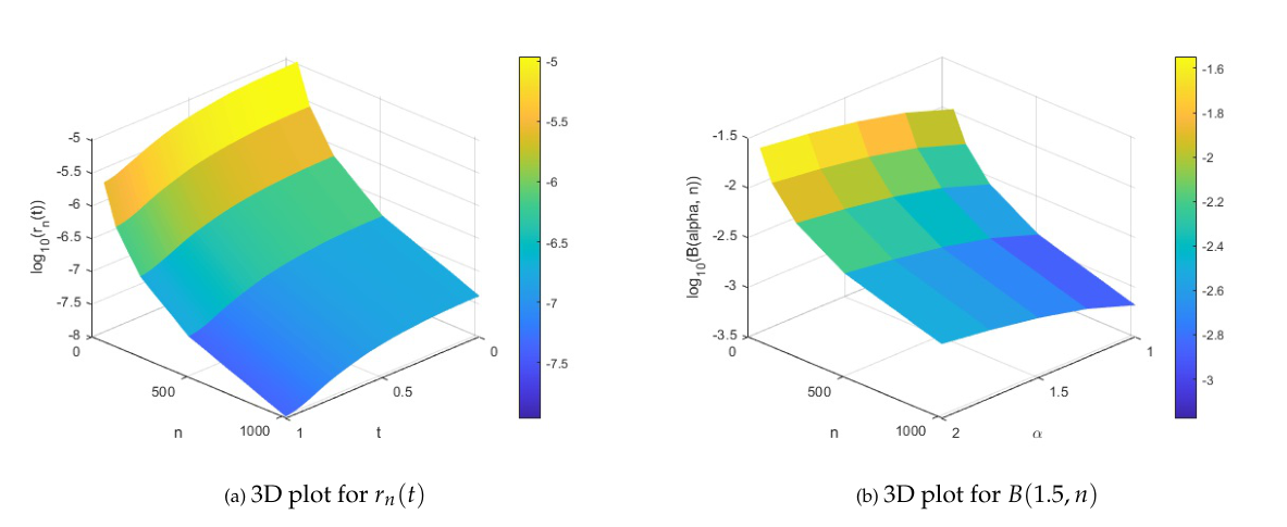
The following is a graphical representation of the accuracy of the approximation for the Fourier transform for various values of \(n\) and \(t \in (0,1]\). Also presented is the bound (33) for the same values of \(n\) and \( \alpha \in (1,2]\).
We can see in Figure 1 that the approximation improves as \(n\) increases. Also, we note that \(B(\alpha ,n)\geq |R_{n}(f,t)|\) as predicted by the theoretical approach. The numerical approximation errors and their corresponding upper bounds are reported in Table 1.
(a) 3D plot for \(r_n(t)\); (b) 3D plot for \(B(1.5,n)\)
| \(\mathbf{t=0.2}\) | \(\mathbf{t=0.4}\) | \(\mathbf{t=0.6}\) | \(\mathbf{t=0.8}\) | \(\mathbf{t=1}\) | \(\mathbf{B(\alpha=1.5,n)}\) | |
|---|---|---|---|---|---|---|
| \(\mathbf{r_{64}}\) | 1.0573e-05 | 9.4081e-06 | 7.3022e-06 | 4.5585e-06 | 2.7599e-06 | 0.020227 |
| \(\mathbf{r_{128}}\) | 2.6433e-06 | 2.3519e-06 | 1.8252e-06 | 1.1392e-06 | 6.8954e-07 | 0.010113 |
| \(\mathbf{r_{256}}\) | 6.6082e-07 | 5.8796e-07 | 4.5628e-07 | 2.8478e-07 | 1.7236e-07 | 0.0050566 |
| \(\mathbf{r_{512}}\) | 1.6521e-07 | 1.4699e-07 | 1.1407e-07 | 7.1192e-08 | 4.3088e-08 | 0.0025283 |
| \(\mathbf{r_{1024}}\) | 4.1301e-08 | 3.6747e-08 | 2.8517e-08 | 1.7798e-08 | 1.0772e-08 | 0.0012642 |
The analytic expression of the Fourier transform for \(f(s)= s+ \cos (\pi s)\) is \[\begin{cases} -\frac{1}{4\,t^2\,\pi ^2}+\frac{{\mathrm{e}}^{-\pi \,t\,2{}\mathrm{i}}\,\left(1+\pi \,t\,2{}\mathrm{i}\right)}{4\,t^2\,\pi ^2}-\frac{t\,\left({\mathrm{e}}^{-\pi \,t\,2{}\mathrm{i}}+1\right)\,2{}\mathrm{i}}{\pi \,\left(2\,t-1\right)\,\left(2\,t+1\right)}, & 0<t\leq1,t\neq\frac{1}{2} \\ & \\ \frac{1}{2} -\frac{2}{\pi ^2}-\frac{i}{\pi },& t=\frac{1}{2}, \end{cases}\]
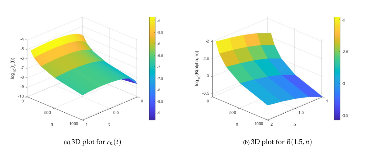
The following provides a graphical representation of the accuracy of the approximation for the Fourier transform for various values of \(n\) and \(t\in (0,1]\). In addition, the corresponding error bound (33) is presented for the same values of \(n\) and \(\alpha \in (1,2]\).
(a) 3D plot for \(r_n(t)\); (b) 3D plot for \(B(1.5,n)\)
As shown in Figure 2, the approximation improves with increasing values of \(n\) . Also, we observe that \(B(\alpha ,n)\geq |R_{n}(f,t)|\). The corresponding numerical approximation errors and upper bounds are reported in Table 2.
| \(\mathbf{t=0.2}\) | \(\mathbf{t=0.4}\) | \(\mathbf{t=0.6}\) | \(\mathbf{t=0.8}\) | \(\mathbf{t=1}\) | \(\mathbf{B(\alpha=1.5,n)}\) | |
|---|---|---|---|---|---|---|
| \(\mathbf{r_{64}}\) | 6.9025e-06 | 1.2182e-05 | 1.4677e-05 | 1.4009e-05 | 1.0657e-05 | 0.0079677 |
| \(\mathbf{r_{128}}\) | 1.7258e-06 | 3.0455e-06 | 3.6691e-06 | 3.5017e-06 | 2.6634e-06 | 0.0039839 |
| \(\mathbf{r_{256}}\) | 4.3145e-07 | 7.6138e-07 | 9.1725e-07 | 8.754e-07 | 6.6581e-07 | 0.0019919 |
| \(\mathbf{r_{512}}\) | 1.0786e-07 | 1.9035e-07 | 2.2931e-07 | 2.1885e-07 | 1.6645e-07 | 0.00099597 |
| \(\mathbf{r_{1024}}\) | 2.6966e-08 | 4.7587e-08 | 5.7328e-08 | 5.4711e-08 | 4.1612e-08 | 0.00049798 |
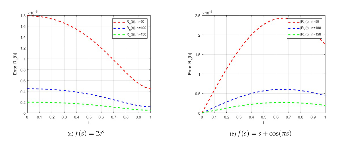
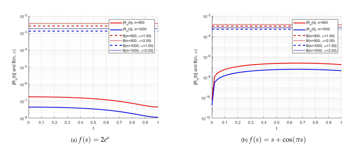
The error curves for both test functions are compared in Figure 3. The corresponding comparisons between the absolute errors and their upper bounds are presented in Figure 4.
(a) \(f(s)=2e^s\); (b) \(f(s)=s+\cos(\pi s)\)
(a) \(f(s)=2e^s\); (b) \(f(s)=s+\cos(\pi s)\)
Remark 5. The plots and tables presented in this section demonstrate that the absolute error \(|R_{n}(f,t)|\) decreases with increasing \(n\). Additionally, we observe that the bound decreases as \(n\) increases. For all the reported numerical results, the absolute error is smaller than the upper bound \(B(\alpha,n)\) when applying equation (32) to approximate the Fourier transform for different functions.