On model for analysis of skeletal muscle contraction

1. Introduction

The prediction and analysis of muscle contraction play a crucial role in understanding the physiological foundations of human movement. Skeletal muscles are central to almost every form of locomotion, and their mechanical behavior significantly impacts clinical assessments, rehabilitation, and athletic performance. In medical contexts, identifying informative parameters of muscle mechanics aids in diagnosing neuromuscular disorders and tailoring treatment regimens for patients undergoing physical therapy or recovery from injury [1– 5].

In sports science, the ability to predict and model muscle behavior enables coaches and trainers to optimize training regimens, enhance athlete performance, and reduce injury risks. The development of accurate biomechanical models helps bridge the gap between theoretical physiology and practical application. With the advancement of real-time data acquisition technologies and simulation tools, modern modeling approaches now allow continuous refinement of treatment and training protocols, even during their active execution. This dynamic adaptability underscores the importance of integrated muscle modeling in both medical and athletic fields.

This paper introduces a mathematical model specifically designed to analyze skeletal muscle contraction while accounting for its deformation properties. Unlike simplified or purely empirical approaches, our model incorporates structural and mechanical aspects of muscle tissue. Furthermore, we present an analytical framework to explore the dynamic behavior of muscle contraction under varying physiological conditions. The proposed approach aims to provide a more realistic representation of muscle function, which can be utilized for both diagnostic and predictive applications in biomedical engineering and sports biomechanics.

2. Method of solution

In this section, we consider the model of skeletal muscle contraction and analyze it. In the framework of the model under consideration, we will assume that the muscle is a locally flat object and has the structure “elastic thread–elastic-viscous substrate”: it is a set of parallel threads connected to an elastic-viscous substrate. We will assume that the effective layer of tissue with depth \(H\) is reduced. A linear law of distribution along the coordinate \(q\) of the component of the displacement field normal to the muscle surface is adopted \[\label{eq:1} U(y,z,t)=V(z,t)\!\left[1+\alpha(y,z,t)\,\frac{y}{z}\right], \tag{1}\] where \(U(y,z,t)\) is the normal-to-surface component of the displacement vector field; \(V(z,t)\) is the movement of a fiber point along the \(O_y\) axis, spaced from the edge at a distance \(z\); \(H\) is the depth of the effective layer of the substrate; \(y\) is the coordinate directed from the free surface of the muscle; \(z\) is the fiber axis coordinate; and \(\alpha\) is the empirical parameter that takes into account possible deviations of the system under consideration from ideality.

The equation of transverse oscillations of a thread on an elastic-viscous substrate has the form [6] \[\label{eq:2} m\,\frac{\partial^2 V(z,t)}{\partial t^2} =\frac{\partial}{\partial z}\!\left(T(y,z,t)\,\frac{\partial V(z,t)}{\partial z}\right)-q(y,z,t), \tag{2}\] where \(m\) is the mass per unit length of the thread; \(T(y,z,t)\) is the thread tension force; and \(q(y,z,t)\) is the distributed shear force from the side of the substrate, directed against the axis \(y\). Force \(q(y,z,t)\) is determined through the tension in the muscle–substrate \(\sigma\), multiplied by the effective width \(b\): \(q=\sigma\,b\).

As boundary conditions, Eq. (2) is supplemented by the conditions for fastening the thread \[ V(0,t) =0,\qquad V(L,t)=0, \label{eq:3a}\ \tag{3a}\] \[V(z,0) =V_0,\qquad \frac{\partial V}{\partial t}(z,0)=0. \label{eq:3b} \tag{3b}\] Here \(L\) is the effective thread length and \(V_0\) is the initial displacement.

We solve (2)–(3) by the method of functional corrections [7, 8]. Within this approach, we represent the thread tension as \[\label{eq:4} T(y,z,t)=T_0\!\left[1+\varepsilon\,g(y,z,t)\right], \qquad 0\le\varepsilon<1,\ \ |g(y,z,t)|\le 1, \tag{4}\] where \(T_0\) is the average value of the tension. We seek the solution in the form of a power series \[\label{eq:5} V(z,t)=\sum_{i=0}^{\infty}\varepsilon^{\,i}\,V_i(z,t). \tag{5}\]

Substituting (4) and (5) into (2)–(3) and grouping terms by powers of \(\varepsilon\) yields problems for \(V_i\): \[ m\,\frac{\partial^2 V_0}{\partial t^2}-T_0\,\frac{\partial^2 V_0}{\partial z^2} =-\,q(y,z,t), \label{eq:6a}\ \tag{6a}\] \[m\,\frac{\partial^2 V_i}{\partial t^2}-T_0\,\frac{\partial^2 V_i}{\partial z^2} = \frac{\partial}{\partial z}\!\left(T_0\,g(y,z,t)\,\frac{\partial V_{i-1}}{\partial z}\right), \qquad i\ge 1, \label{eq:6b} \tag{6b}\] with boundary and initial conditions \[\label{eq:7} V_i(0,t)=0,\ \ V_i(L,t)=0,\ \ \frac{\partial V_i}{\partial t}(z,0)=0\ (i\ge 0);\qquad V_0(z,0)=V_0,\ \ V_i(z,0)=0\ (i\ge 1). \tag{7}\]

Eqs. (6)–(7) are solved by Fourier separation of variables [9]. The solutions can be written as sine-series over the eigenfunctions \(\sin\!\big(\tfrac{n\pi z}{L}\big)\): \[ V_0(z,t) =\sum_{n=1}^{\infty}\sin\!\Big(\frac{n\pi z}{L}\Big)\! \left[ A_n\cos(\omega_n t)+B_n\sin(\omega_n t) +\frac{1}{m}\int_0^t \hat q_n(\tau)\,\frac{\sin\!\big(\omega_n(t-\tau)\big)}{\omega_n}\,d\tau \right], \label{eq:8}\ \tag{8a}\][4pt] \[V_i(z,t) =\frac{T_0}{m}\sum_{n=1}^{\infty}\sin\!\Big(\frac{n\pi z}{L}\Big)\! \int_0^t \widehat{\mathcal{G}}_{n,i}(\tau)\,\frac{\sin\!\big(\omega_n(t-\tau)\big)}{\omega_n}\,d\tau,\qquad i\ge 1, \ \tag{8b}\] where \(\omega_n=\sqrt{\tfrac{T_0}{m}}\,\tfrac{n\pi}{L}\), \(\hat q_n(t)=\tfrac{2}{L}\int_0^L q(y,\zeta,t)\sin\!\big(\tfrac{n\pi\zeta}{L}\big)\,d\zeta\), and \[\widehat{\mathcal{G}}_{n,i}(t)=\frac{2}{L}\int_0^L \frac{\partial}{\partial \zeta}\!\left[g(y,\zeta,t)\,\frac{\partial V_{i-1}}{\partial \zeta}(\zeta,t)\right]\sin\!\Big(\frac{n\pi\zeta}{L}\Big)\,d\zeta.\]

Constants \(A_n\) and \(B_n\) are fixed by the initial data (7). The spatio-temporal distributions \(V(z,t)\) were analyzed analytically by using the second-order (\(i=0,1,2\)) approximation in the framework of the method of functional corrections. This approximation is usually sufficiently accurate for qualitative analysis and to obtain some quantitative results. All obtained results have been checked by comparison with results of numerical simulations.

3. Discussion

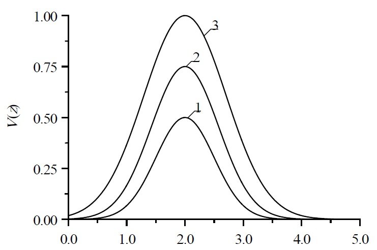
In this section, we analyze the spatio-temporal distribution of the fiber-point displacement along the \(O_y\) axis. Figure 1 shows typical dependences of the considered distribution on the coordinate during fiber compression for various values of the external force \(q\). An increase in the curve number corresponds to an increase in the considered force. Stretching the fiber leads to the opposite result. A similar result was obtained when analyzing the change in fiber over time.

4. Conclusion

In this paper, we propose a model for the analysis of skeletal muscle contraction, which takes into account its deformation properties. We analyzed the considered model. We introduce an analytical approach for analysis of the considered muscle contraction.