
1. Introduction
Viral conjunctivitis is a common cause of infectious red eye and encompasses clinically and epidemiologically distinct conditions. Adenoviruses account for a large share of viral conjunctivitis, while acute haemorrhagic conjunctivitis (AHC) is commonly associated with enterovirus 70 and coxsackievirus A24 variant [1,2]. AHC is especially relevant to outbreak modeling because it has a short incubation period, high transmissibility, and the capacity to spread rapidly in schools and other settings with frequent close contact [3–5]. These features make early contact reduction, hygiene, surveillance, diagnosis, and removal from infectious contact plausible components of outbreak control.
Previous mathematical studies have examined conjunctivitis transmission using compartmental models, quarantine, isolation, treatment, education, and optimal-control formulations [4,6–9]. This literature demonstrates the value of mathematical thresholds, but it also shows why intervention parameters must be clearly defined. A dimensionless reduction in contact cannot be compared directly with a removal rate unless their mechanisms, units, and admissible ranges are specified. Likewise, a controlled reproduction number evaluated at a disease-free state is not identical to a time-dependent effective reproduction number, which also depends on the susceptible fraction.
The present study addresses these issues with four contributions. First, it uses a closed-population SEIR outbreak model whose incidence and transition terms are dimensionally consistent and whose feasible region is positively invariant. Second, it derives the basic, controlled, and state-dependent effective reproduction numbers from the infected subsystem using the next-generation-matrix method [10,11]. Third, it identifies the complete threshold curve separating invasion from decline under contact reduction and treatment-supported case management. Fourth, it evaluates representative intervention scenarios with reproducible ordinary differential equation simulations, a 10,000-draw parameter uncertainty analysis, mass-balance tests, and cross-solver numerical verification.
The analysis is deliberately framed as an outbreak scenario rather than an empirical forecast for a particular country. The baseline transmissibility and natural-history values are anchored to published AHC estimates [3], whereas the maximum additional removal rate attributable to case management is treated as an explicit scenario parameter and varied over a broad range. This separation prevents an assumed operational parameter from being presented as a measured clinical effect.
2. Materials and methods
2.1. Conjunctivitis model without control measures
Let \(S(t)\), \(E(t)\), \(I(t)\), and \(R(t)\) denote the numbers of susceptible, exposed but not yet infectious, infectious, and removed individuals at time \(t\), respectively. The total population is
Because acute conjunctivitis outbreaks typically unfold over weeks rather than decades, births, natural deaths, and waning immunity are omitted. This short-horizon assumption avoids introducing demographic rates that are neither identifiable nor influential on the outbreak time scale. Homogeneous mixing is assumed, and all exposed individuals eventually become infectious. Figure 1 summarizes the transitions.

The corresponding equations are
Here \(\beta\) is the effective transmission coefficient, \(\sigma^{-1}\) is the mean latent period, and \(\gamma^{-1}\) is the mean duration of infectious contact. Every term in Eq. (1) has units of persons per day.
Adding the equations gives
so \(N(t)=N(0)=N\). On any coordinate boundary, the derivative of the corresponding compartment is nonnegative: for example, \(dE/dt=\beta SI/N\geq0\) when \(E=0\), and \(dI/dt=\sigma E\geq0\) when \(I=0\). Therefore the biologically feasible region
is positively invariant, and all solutions beginning in \(\Omega\) remain nonnegative and bounded. The infection-free state used for invasion analysis is
In a closed outbreak model there is no demographic endemic equilibrium with a constant positive infectious population; instead, the epidemic terminates on the infection-free set \(E=I=0\) after susceptible depletion and removal.
Table 1 lists the baseline values. Chowell et al. estimated that a primary infectious AHC case generated approximately \(2.64\) secondary cases, with standard deviation \(0.65\), in the 2003 Mexico outbreak [3]. The same outbreak literature reports an incubation period of approximately 1–2 days and an infectious period of approximately 3–7 days; their midpoints give \(\sigma=1/1.5=0.6667\) day\(^{-1}\) and \(\gamma=1/5=0.2000\) day\(^{-1}\). We set \(\beta=R_0\gamma=0.5280\) day\(^{-1}\). The value \(\tau=0.25\) day\(^{-1}\) is an operational scenario assumption, not a drug-efficacy estimate, and is varied from \(0.15\) to \(0.35\) day\(^{-1}\) in uncertainty analysis.
| Symbol | Interpretation | Baseline value | Units or source |
|---|---|---|---|
| \(N\) | Size of the illustrative closed cohort | \(10{,}000\) | persons; scenario |
| \(\beta\) | Effective transmission coefficient | \(0.5280\) | day\(^{-1}\); calibrated from [3] |
| \(\sigma\) | Progression rate from exposed to infectious | \(0.6667\) | day\(^{-1}\); 1.5-day mean [3] |
| \(\gamma\) | Baseline removal rate from infectious contact | \(0.2000\) | day\(^{-1}\); 5-day mean [3] |
| \(\tau\) | Maximum additional removal rate under case management | \(0.2500\) | day\(^{-1}\); scenario range \(0.15\)–\(0.35\) |
| \(u_1\) | Proportional reduction in effective contact | \([0,1]\) | dimensionless control |
| \(u_2\) | Intensity of treatment-supported case management | \([0,1]\) | dimensionless control |
2.2. Basic reproduction number
The infected-state vector is \(x=(E,I)^{\mathsf T}\). At \(\mathcal{E}_0\), the new-infection and transition matrices are
Thus
The latent rate \(\sigma\) does not appear in \(R_0\) because, under the stated assumptions, every exposed individual survives the latent stage and enters the infectious class. Substituting the baseline values gives \(R_0=0.5280/0.2000=2.64\), consistent by construction with the published AHC estimate.
2.3. Conjunctivitis model with control measures
Two controls are distinguished mechanistically. The contact-reduction control \(u_1\in[0,1]\) is the proportional decrease in effective infectious contacts associated with measures such as hand hygiene, environmental disinfection, reduced close contact, and adherence to separation guidance. The case-management control \(u_2\in[0,1]\) represents prompt identification and treatment-supported removal from infectious contact. It is not interpreted as a direct antiviral cure. Its maximum additional removal rate is \(\tau\), so its dimensional contribution is \(\tau u_2\) day\(^{-1}\). Figure 2 shows the controlled flows.

The controlled system is
The conservation and positivity arguments used for the uncontrolled system remain valid for every admissible pair \((u_1,u_2)\in[0,1]^2\).
2.4. Controlled and effective reproduction numbers
For constant control levels, the next-generation construction applied to Eq. (7) gives
and hence
The required consistency identity follows immediately:
The state-dependent effective reproduction number is
Unlike \(R_c\), which is an invasion threshold at the fully susceptible state, \(R_e(t)\) decreases as susceptible individuals are removed.
The Jacobian of the infected subsystem \((E,I)\) at \(\mathcal{E}_0\) has characteristic polynomial
Both Routh–Hurwitz coefficients are positive when \(R_c<1\), so the infection-free state is locally asymptotically stable in the infected directions. When \(R_c>1\), the constant term is negative and one eigenvalue is positive; invasion is then possible.
Solving \(R_c=1\) gives the threshold curve
Equivalently, for a fixed \(u_1\), case management must satisfy
whenever the right-hand side is positive.
3. Results and discussion
3.1. Numerical simulations
The controlled system was solved over 120 days for an illustrative cohort of \(N=10{,}000\) with
The primary calculations used the DOP853 method with relative tolerance \(10^{-10}\), absolute tolerance \(10^{-12}\), and maximum internal step \(0.05\) day. Recalculation with RK45, tighter reference tolerances, and a \(0.025\)-day maximum step was used for numerical verification. The complete Python script, random seed, PNG files, and numerical summaries accompany the manuscript.
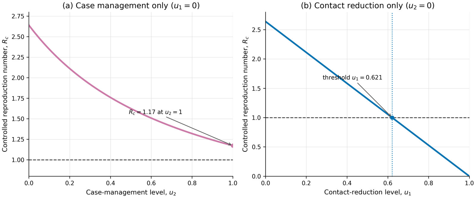
Figure 3(a) shows that case management alone decreases \(R_c\) monotonically from \(2.64\) at \(u_2=0\) to \(1.173\) at \(u_2=1\). Under the assumed maximum additional removal rate, it cannot reduce the invasion number below one by itself. This does not mean that case management is ineffective: it reduces the simulated peak and attack rate substantially, but its baseline parameterization is insufficient for prevention of invasion when used alone. Figure 3(b) shows the linear effect of contact reduction. The exact contact-only threshold is
Therefore \(u_1>0.6212\) gives \(R_c<1\) at the baseline parameter values.
Four dynamic scenarios were examined: no control \((0,0)\); contact reduction only \((0.65,0)\); case management only \((0,0.80)\); and combined controls \((0.50,0.80)\). Their controlled reproduction numbers are \(2.640\), \(0.924\), \(1.320\), and \(0.660\), respectively. As shown in Figure 4(a), the uncontrolled scenario peaks at \(1934.952\) infectious individuals on day \(34.45\) and generates new infections in \(90.938\%\) of initially susceptible individuals by day 120. Contact reduction alone produces a much smaller transient peak of \(11.028\) infectious individuals on day \(4.40\) and a \(1.312\%\) attack rate. Case management alone delays and reduces the epidemic, but because \(R_c=1.320>1\), it still produces a peak of \(207.467\) infectious individuals on day \(60.45\) and a \(43.988\%\) attack rate. The combined scenario gives a peak of \(8.156\) infectious individuals on day \(1.95\) and a \(0.289\%\) attack rate.
Figure 4(b) distinguishes the time-dependent \(R_e(t)\) from the constant invasion value \(R_c\). For the contact-only and combined scenarios, \(R_e(t)<1\) from the start. For the uncontrolled and case-management-only scenarios, susceptible depletion eventually pushes \(R_e(t)\) below one, but only after substantial transmission. This timing explains why crossing below one late in an outbreak cannot be interpreted as successful early prevention.
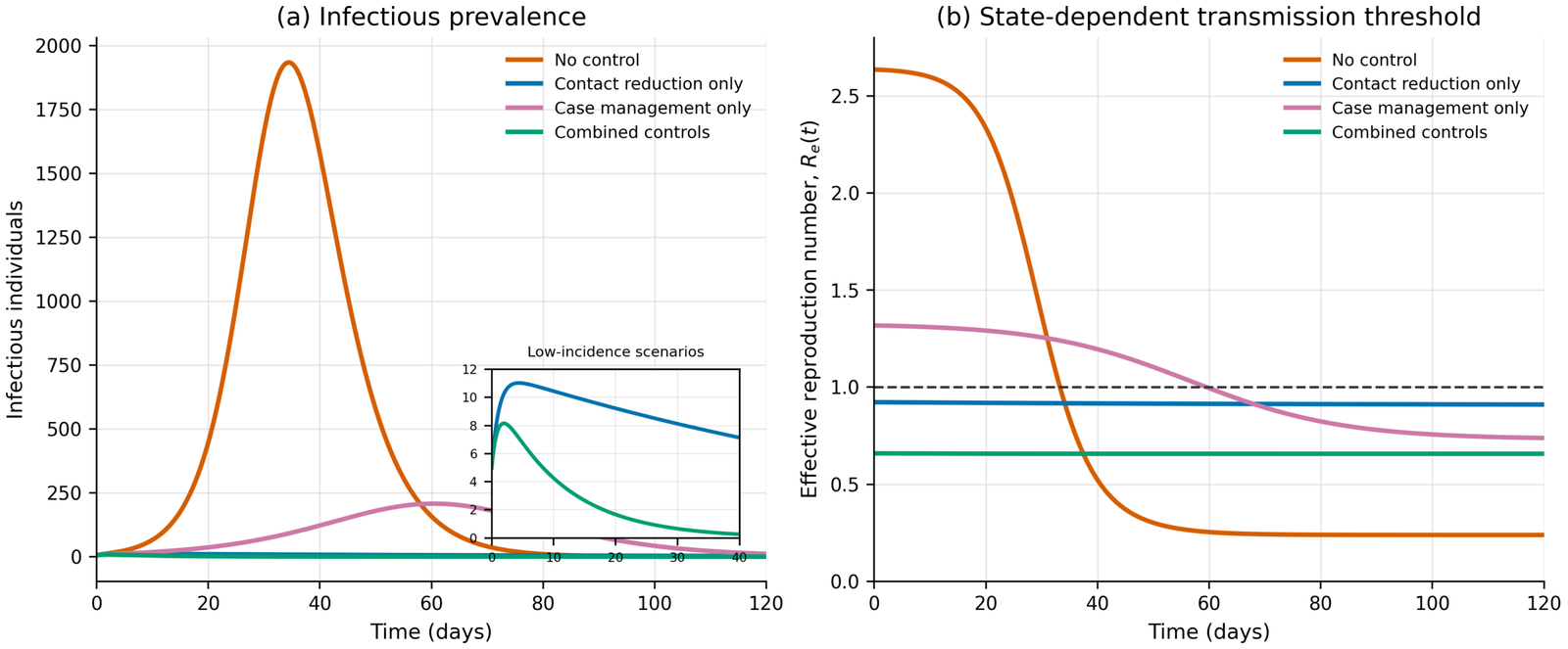
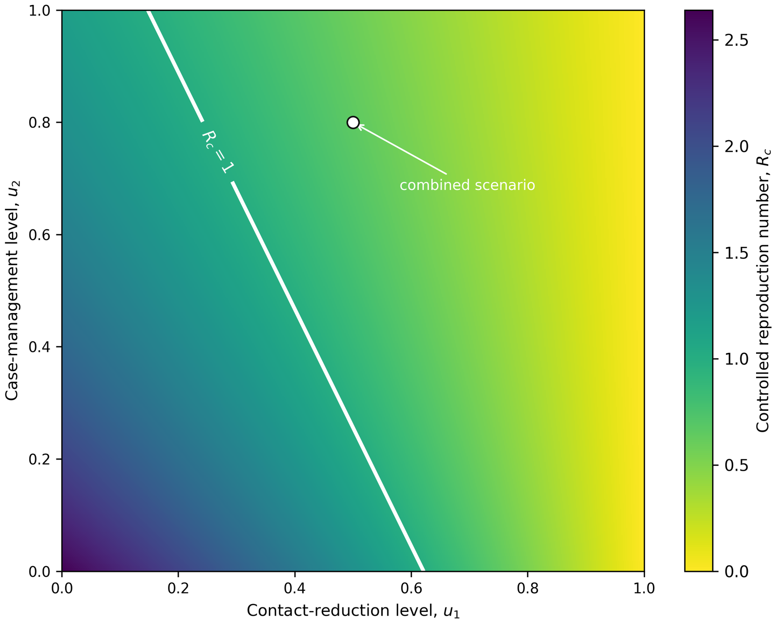
Figure 5 displays \(R_c\) over the full admissible control square. The white contour is the analytic boundary from Eq. (12); points to its upper-right satisfy \(R_c<1\). At \(u_2=0.80\), the minimum contact reduction required by the baseline parameters is \(u_1>0.2424\). Conversely, at \(u_1=0.50\), the minimum case-management level is \(u_2>0.2560\). The selected combined point \((0.50,0.80)\) lies well inside the \(R_c<1\) region and gives \(R_c=0.660\).
Parameter uncertainty was evaluated with 10,000 Monte Carlo draws using the fixed random seed 20260725. The published reproduction-number estimate was represented by a normal distribution with mean \(2.64\) and standard deviation \(0.65\), truncated to \([1.1,5.0]\); the infectious period was sampled uniformly from 3 to 7 days; and \(\tau\) was sampled uniformly from \(0.15\) to \(0.35\) day\(^{-1}\). For each draw, \(\gamma\) was the reciprocal of the sampled infectious period and \(\beta=R_0\gamma\). The no-control median was \(2.645\) with a \(95\%\) simulation interval of \(1.463\)–\(3.906\). The contact-only scenario had median \(R_c=0.926\) (\(95\%\) interval \(0.512\)–\(1.367\)) and \(P(R_c<1)=0.631\). The case-management-only scenario had median \(1.322\) (\(95\%\) interval \(0.679\)–\(2.215\)) and \(P(R_c<1)=0.183\). The combined scenario had median \(0.661\) (\(95\%\) interval \(0.339\)–\(1.108\)) and \(P(R_c<1)=0.939\). These intervals show that threshold conclusions close to one are sensitive to uncertain operational effectiveness; the combined strategy is more robust in this parameter space, but not guaranteed under every draw.
The numerical implementation passed three internal validation tests. First, \(R_c(0,0)-R_0\) was zero to machine precision. Second, the maximum population-balance error across all scenarios was \(7.64\times10^{-11}\) persons, and no compartment became negative. Third, the maximum absolute difference between the DOP853 and RK45 solutions was \(4.35\times10^{-10}\) persons. These checks establish computational reproducibility and internal consistency, although they are not a substitute for validation against independent outbreak data.
The model has several limitations. Homogeneous mixing ignores household, classroom, age, and spatial structure. Controls are constant within each scenario, whereas adherence and implementation often change after outbreak recognition. The exposed class is assumed noninfectious, all exposed individuals progress to infectiousness, and the case-management rate \(\tau\) is scenario-based rather than estimated from patient-level data. Environmental persistence and indirect transmission are absorbed into \(\beta\) rather than represented by a separate reservoir. Finally, the calibration is based on AHC evidence and should not be transferred without adjustment to adenoviral or other viral conjunctivitis syndromes with different natural histories. For application to a specific population, the model should be fitted to local onset data and accompanied by identifiable intervention dates, reporting corrections, and out-of-sample assessment.
4. Conclusion
A dimensionally consistent SEIR formulation yields clear distinctions among \(R_0\), the controlled invasion number \(R_c\), and the state-dependent effective number \(R_e(t)\). Under the baseline AHC calibration, contact reduction alone crosses the invasion threshold at \(u_1=0.621\), the assumed case-management range does not cross it alone, and the combined scenario \((0.50,0.80)\) gives \(R_c=0.660\). Dynamic simulations, uncertainty analysis, mass conservation, and cross-solver agreement support the internal validity of these results. The findings indicate complementarity between contact reduction and prompt case management, rather than a universal ranking of one intervention above the other. Population-specific recommendations require local calibration and empirical estimates of intervention effectiveness.
Author Contributions: Conceptualization, V.M. and C.U.; methodology, V.M., H.R., J.U.R., and L.T.; software, V.M. and C.U.; investigation, P.N. and J.U.R.; writing—original draft preparation, V.M. and P.N.; writing—review and editing, P.N. and C.U.; visualization, V.M., J.U.R., and P.N.; supervision, H.R. and L.T. All authors have read and agreed to the submitted version of the manuscript.
Funding Information: This research received no external funding.
Conflicts of Interest: The authors declare no conflict of interest.
Data Availability: No new patient-level data were used. The complete simulation code, fixed random seed, generated PNG figures, scenario summaries, uncertainty output, and numerical validation results are included with the LaTeX source.