
In recent years, the study of traveling wave solutions, particularly in models involving competing species, has attracted significant interest. A notable nonlocal example appears in the work of Dong, Li, and Zhang [1], where the existence of traveling waves is considered for the following Leslie-Gower predator-prey model with nonlocal dispersal: \[\begin{aligned} \frac{\partial u(x,t)}{\partial t} &= (J_1 * u)(x,t) – u(x,t) + ru(x,t)\left(1 – u(x,t) – kv(x,t)\right), \\ \frac{\partial v(x,t)}{\partial t} &= (J_2 * v)(x,t) – v(x,t) + sv(x,t)\left(1 – \frac{v(x,t)}{u(x,t)}\right). \end{aligned}\]
This model describes a system in which the predator depends entirely on the prey for survival. As a result, when the prey density is small relative to that of the predator, the predator population is expected to decline toward extinction. However, the responses of predator and prey populations are not instantaneous. In particular, maturation delays and delayed responses to environmental changes can significantly affect the long-term dynamics, including persistence or extinction.
The existence of traveling wave solutions for models with delays in the reaction terms has been studied in [2– 5]. In those works, the reaction terms satisfy either monotone or exponentially quasi-monotone conditions. However, in the context of competition models, the reaction terms typically satisfy only partial monotonicity or exponentially quasi-monotone conditions, as discussed in [6].
More recently, the incorporation of spatial delays into traveling wave models has been investigated. When delay is present in the diffusion term, the existence of traveling wave solutions has been established in [7– 12]. For models with nonlocal diffusion and delay, the existence of traveling waves has been shown by Jiang and Yang [13].
In the case of predator-prey models with delay in the reaction term and local, non-delayed diffusion, traveling wave solutions have been established in [14– 16]. When no delay is present and the diffusion is nonlocal, existence results are found in [1, 17, 18].
For further background on traveling waves and competitive diffusive models, the reader is referred to [19– 25].
In this paper we establish traveling waves for the following Leslie-Gower model with nonlocal dispersal terms with delay.
\[\begin{aligned} \label{PDE1} \frac{\partial u_1}{\partial t}(t,x) =& \int_{-\infty}^{\infty} J_1(y)\,\Bigl[u_1\bigl(t-\tau_1,\,x-y\bigr)\;-\;u_1\bigl(t-\tau_1,\,x\bigr)\Bigr]\,dy +\;\alpha_1\,u_1(t,x)\,\Bigl[1 \;-\;u_1(t,x)\;-\;k\,u_2\bigl(t-\tau_2,\,x\bigr)\Bigr] \nonumber \\ \frac{\partial u_2}{\partial t}(t,x) =& \int_{-\infty}^{\infty} J_2(y)\,\Bigl[u_2\bigl(t-\tau_3,\,x-y\bigr)\;-\;u_2\bigl(t-\tau_3,\,x\bigr)\Bigr]\,dy +\;\alpha_2\,u_2(t,x)\,\Bigl[1 \;-\;\frac{u_2(t,x)}{u_1\bigl(t-\tau_4,\,x\bigr)}\Bigr]. \end{aligned} \tag{1}\]
We impose the following for \(i \in \{1, 2\}\), \(J_i\) satisfies
(J1) \(J_i(x) > 0\), for all \(x\in\mathbb{R}\).
(J2) \(\int_{\mathbb{R}}J_i(x)dx = 1\).
(J3) \(\int_{\mathbb{R}}J_i(x)e^{\mu|x|}dx < \infty\) for all \(\mu \in \mathbb{R}\).
Assuming \(u_i(x,t)=\phi_i(t), \xi=x+ct.\) Here, we use the vvariable \(t\) instead of \(\xi\) for convenience. we see the system (1) becomes
\[\begin{aligned} \label{wave1} c\,\phi_1'(t) &= \int_{-\infty}^{\infty} J_1(y)\,\Bigl[\phi_1(t – y -c\,\tau_1) \;-\;\phi_1(t -c\,\tau_1)\Bigr]\,dy \;+\;\alpha_1\,\phi_1(t)\,\Bigl[1 \;-\;\phi_1(t)\;-\;k\,\phi_2(t -c\,\tau_2)\Bigr], \nonumber\\[6pt] c\,\phi_2'(t) &= \int_{-\infty}^{\infty} J_2(y)\,\Bigl[\phi_2(t – y -c\,\tau_3) \;-\;\phi_2(t -c\,\tau_3)\Bigr]\,dy \;+\;\alpha_2\,\phi_2(t)\,\Bigl[1 \;-\;\frac{\phi_2(t)}{\phi_1(t -c\,\tau_4)}\Bigr]. \end{aligned} \tag{2}\]
This manuscript is organized as follows. In §2, we provide preliminary information and introduce notation. In §3, we establish the existence of traveling wave solutions for competition models under a partial monotonicity condition. Our approach is based on the construction of upper and lower solutions and the development of an iterative operator that maps into a suitable set, with existence guaranteed by Schauder’s fixed point theorem. We then extend the framework to accommodate a relaxed class of super- and sub-solutions. In §4, we present explicit constructions of such solutions, along with a proof of the existence of a coexistence state and numerical illustrations demonstrating up to fifty iterations.
In this paper, we adopt the standard notations \(\mathbb{R}^n\) and \(\mathbb{C}^n\) for the real and complex vector spaces of dimension \(n\). We also use the standard partial ordering on \(\mathbb{R}^2\): for vectors \(u = (u_1, u_2)^T\) and \(v = (v_1, v_2)^T\), we write \(u \leq v\) if \(u_1 \leq v_1\) and \(u_2 \leq v_2\), and \(u < v\) if \(u_1 < v_1\) and \(u_2 < v_2\). The Euclidean norm in \(\mathbb{R}^2\) is denoted by \(|\cdot|\).
The space of all bounded and continuous functions from \(\mathbb{R} \to \mathbb{R}^n\) is denoted by \(BC(\mathbb{R}, \mathbb{R}^n)\), equipped with the sup-norm \[\| f \| := \sup_{t \in \mathbb{R}} | f(t) |,\] where \(f(t) \in C(U, \mathbb{R}^2)\) for some \(U \subset \mathbb{R}\). The space \(BC^k(\mathbb{R}, \mathbb{R}^n)\) consists of all \(k\)-times continuously differentiable functions from \(\mathbb{R} \to \mathbb{R}^n\) whose derivatives up to order \(k\) are bounded.
If boundedness is not required, we write \(C(\mathbb{R}, \mathbb{R}^n)\) and \(C^k(\mathbb{R}, \mathbb{R}^n)\) for the corresponding function spaces. For \(f, g \in BC(\mathbb{R}, \mathbb{R}^n)\), we write \(f \leq g\) if and only if \(f(t) \leq g(t)\) for all \(t \in \mathbb{R}\). A constant function \(f(t) = \alpha\) for all \(t \in \mathbb{R}\) is denoted by \(\hat{\alpha}\).
An operator \(P\) acting on a subset \(S \subset BC(\mathbb{R}, \mathbb{R}^2)\) is said to be monotone if \(f \leq g\) implies \(Pf \leq Pg\) for all \(f, g \in S\). In particular, if \(P\) is linear and defined on all of \(BC(\mathbb{R}, \mathbb{R}^2)\), then \(P\) is monotone if and only if it maps nonnegative functions to nonnegative functions.
We now recall standard definitions of function spaces that will be used throughout this work.
Definition 1(\(L^p\) Spaces). Let \(n \in \mathbb{N}\). For \(1 \leq p \leq \infty\), the space \(L^p(\mathbb{R}, \mathbb{R}^2)\) consists of all measurable functions \(f \colon \mathbb{R} \to \mathbb{R}\) such that \[\| f \|_{L^p} = \begin{cases} \left( \displaystyle\int_{\mathbb{R}} |f(x)|^p \, dx \right)^{1/p}, & 1 \leq p < \infty, \\[6pt] \displaystyle \operatorname{ess\,sup}_{x \in \mathbb{R}} |f(x)|, & p = \infty, \end{cases}\] is finite.
Definition 2(Sobolev Space \(W^1,^p\)).For \(1 \leq p \leq \infty\), the Sobolev space \(W^{1,p}(\mathbb{R}, \mathbb{R}^2)\) is defined as \[W^{1,p}(\mathbb{R}, \mathbb{R}^2) = \left\{ f \in L^p(\mathbb{R}, \mathbb{R}^2) \;\middle|\; f \text{ is absolutely continuous and } f' \in L^p(\mathbb{R}, \mathbb{R}^2) \right\}.\]
This space is continuously embedded in \(L^\infty(\mathbb{R}, \mathbb{R}^2)\); that is, there exists a constant \(C > 0\) such that \[\| f \|_{L^\infty} \leq C \| f \|_{W^{1,p}} \quad \text{for all } f \in W^{1,p}(\mathbb{R}, \mathbb{R}^2).\]
Definition 3(Sobolev Space \(W^2,infinity\)).The Sobolev space \(W^{2,\infty}(\mathbb{R}, \mathbb{R}^2)\) is defined by \[W^{2,\infty}(\mathbb{R}, \mathbb{R}^2) = \left\{ f \in L^\infty(\mathbb{R}, \mathbb{R}^2) \;\middle|\; f' \in L^\infty(\mathbb{R}, \mathbb{R}^2),\, f' \text{ is absolutely continuous, and } f'' \in L^\infty(\mathbb{R}, \mathbb{R}^2) \right\}.\]
Equivalently,
\[W^{2,\infty}(\mathbb{R}, \mathbb{R}^2) = \left\{ f \in W^{1,\infty}(\mathbb{R}, \mathbb{R}^2) \;\middle|\; f' \in W^{1,\infty}(\mathbb{R}, \mathbb{R}^2) \right\}.\]
Finally, we define the function \[f_{ic}(\phi_\theta, \psi_\theta): \mathcal{X}_{c\tau} := C([-\tau, 0], \mathbb{R}^2) \to \mathbb{R}, \quad \text{where } \tau = \max\{\tau_j : j = 1, \dots, 6\},\] by \[f_{ic}(\phi, \psi) = f_i(\phi^c, \psi^c), \quad \phi^c(\theta) = \phi(c\theta), \quad \psi^c(\theta) = \psi(c\theta), \quad \theta \in [-\tau, 0], \quad i = 1, 2,\] which gives the following form of the wave system. \[\begin{aligned} \label{wave2} c\,\phi_1'(t) &= \int_{-\infty}^{\infty} J_1(y)\,\Bigl[\phi_1(t – y -c\,\tau_1) \;-\;\phi_1(t -c\,\tau_1)\Bigr]\,dy \;+f_{1c}(\phi_t, \psi_t), \nonumber\\[6pt] c\,\phi_2'(t) &= \int_{-\infty}^{\infty} J_2(y)\,\Bigl[\phi_2(t – y -c\,\tau_3) \;-\;\phi_2(t -c\,\tau_3)\Bigr]\,dy \;+f_{2c}(\phi_t, \psi_t). \end{aligned} \tag{3}\]
In this section, we begin by developing a cross iteration method. We start by defining the following functions:
\[\begin{aligned} H_1(\Phi)(t) &= \int_{-\infty}^{\infty} J_1(y) \left[ \phi_1(st – y – c\tau_1) – \phi_1(t – c\tau_1) \right] dy + \alpha_1 \phi_1(t) \left[ 1 – \phi(t) – k\phi_2(t – c\tau_2) \right] + \beta_1 \phi_1(t), \\ H_2(\Phi)(t) &= \int_{-\infty}^{\infty} J_2(y) \left[ \phi_2(t – y – c\tau_3) – \phi_2(t – c\tau_3) \right] dy + \alpha_2 \phi_2(t) \left[ 1 – \frac{\phi_2(t)}{\phi_1(t – c\tau_4)} \right] + \beta_2 \phi_2(t), \end{aligned}\] for some \(\beta_1, \beta_2 > 0\), and where \(\Phi = (\phi_1, \phi_2)\).
Then, the system (2) is equivalent to \[\phi_i(t) = \frac{1}{c} \cdot e^{\frac{-\beta_1}{c} t} \cdot \int_{-\infty}^{t} \left( H_i(\Phi)(s) \cdot e^{\frac{\beta_1}{c} s} \right) ds.\]
We develop sufficient conditions for the existence of traveling wave solutions for equations of the form (2). We invoke the following cross iteration scheme. First, assume:
1. \(f(\hat{0}) = f(\hat{K}) = 0\), where \(K = (k_1, k_2)\).
2. There exist two positive Lipschitz constants \(L_1, L_2\) such that \[\begin{aligned} \left| f_1(\Phi) – f_1(\Psi) \right| &\leq L_1 \left\| \Phi – \Psi \right\|, \\ \left| f_2(\Phi) – f_2(\Psi) \right| &\leq L_2 \left\| \Phi – \Psi \right\|, \end{aligned}\] for \(\Phi, \Psi \in C\left([-\tau, 0], \mathbb{R}\right)\), with \(\tau = \max\{\tau_j : j = 1,2,3,4\}\).
Definition 4(Partial Quasi-Monotone Condition (PQM)).Fix two constants \(\beta_1, \beta_2 > 0\) such that:
1. \(f_1(\phi_1(s), \psi_1(s)) – f_1(\phi_2(s), \psi_1(s)) + \beta_1 [\phi_1(0) – \phi_2(0)] \geq 0,\)
2. \(f_1(\phi_1(s), \psi_1(s)) – f_1(\phi_1(s), \psi_2(s)) \leq 0,\)
3. \(f_2(\phi_1(s), \psi_1(s)) – f_2(\phi_2(s), \psi_2(s)) + \beta_2 [\psi_1(0) – \psi_2(0)] \geq 0,\) where \[1 – k \leq \phi_2 \leq \phi_1 \leq 1, \quad 0 \leq \psi_2 \leq \psi_1 \leq 1.\]
Theorem 1. There exist two positive numbers \(\beta_1 > 0, \beta_2 > 0\) such that \[1 – k \leq \phi_2 \leq \phi_1 \leq 1, \quad 0 \leq \psi_2 \leq \psi_1 \leq 1,\] and the following identities hold: \[\begin{aligned} f_1(\phi_1(s), \psi_1(s)) &= \alpha_1 \phi_1(0) \left[ 1 – \phi_1(0) – k\psi_1(-c\tau_2) \right], \\ f_1(\phi_1(s), \psi_2(s)) &= \alpha_1 \phi_1(0) \left[ 1 – \phi_1(0) – k\psi_2(-c\tau_2) \right], \\ f_2(\phi_1(s), \psi_1(s)) &= \alpha_2 \psi_1(0) \left[ 1 – \frac{\psi_1(0)}{\phi_1(-c\tau_4)} \right], \\ f_2(\phi_2(s), \psi_2(s)) &= \alpha_2 \psi_2(0) \left[ 1 – \frac{\psi_2(0)}{\phi_2(-c\tau_4)} \right], \end{aligned}\] which satisfy the Partial Quasi-Monotone Condition (PQM).
Proof. We begin with the first inequality: \[\begin{aligned} f_1(\phi_1, \psi_1) – f_1(\phi_2, \psi_1) &= \alpha_1 \phi_1(0)[1 – \phi_1(0) – k \psi_1(-c\tau_2)] – \alpha_1 \phi_2(0)[1 – \phi_2(0) – k \psi_1(-c\tau_2)] \\ &= \alpha_1 \phi_1(0) – \alpha_1 \phi_2(0) – \alpha_1 \phi_1^2(0) + \alpha_1 \phi_2^2(0) – \alpha_1 k \psi_1(-c\tau_2)[\phi_1(0) – \phi_2(0)] \\ &= \alpha_1[\phi_1(0) – \phi_2(0)]\left[1 – (\phi_1(0) + \phi_2(0)) – k \psi_1(-c\tau_2)\right] \\ &\ge \alpha_1[\phi_1(0) – \phi_2(0)](1 – 2 – k) \\ &= -\alpha_1(1 + k)[\phi_1(0) – \phi_2(0)]. \end{aligned}\]
Thus, \[f_1(\phi_1(s), \psi_1(s)) – f_1(\phi_2(s), \psi_1(s)) + \beta_1[\phi_1(0) – \phi_2(0)] \ge 0\] whenever \[\beta_1 \ge \alpha_1(1 + k).\]
Next, for the second inequality: \[\begin{aligned} f_1(\phi_1, \psi_1) – f_1(\phi_1, \psi_2) &= \alpha_1 \phi_1(0)[1 – \phi_1(0) – k \psi_1(-c\tau_2)] – \alpha_1 \phi_1(0)[1 – \phi_1(0) – k \psi_2(-c\tau_2)] \\ &= -\alpha_1 k \phi_1(0)[\psi_1(-c\tau_2) – \psi_2(-c\tau_2)] \le 0. \end{aligned}\]
Now consider the third inequality: \[\begin{aligned} f_2(\phi_1(0), \psi_1(0)) – f_2(\phi_2(0), \psi_2(0)) &= \alpha_2 \psi_1(0)\left[1 – \frac{\psi_1(0)}{\phi_1(-c\tau)}\right] – \alpha_2 \psi_2(0)\left[1 – \frac{\psi_2(0)}{\phi_2(-c\tau)}\right] \\ &= \alpha_2\left[ (\psi_1(0) – \psi_2(0)) – \left(\frac{\psi_1^2(0)}{\phi_1(-c\tau)} – \frac{\psi_2^2(0)}{\phi_2(-c\tau)}\right) \right] \\ &= \alpha_2\left[ (\psi_1(0) – \psi_2(0)) – \frac{\psi_1^2(0)\phi_2(-c\tau) – \psi_2^2(0)\phi_1(-c\tau)}{\phi_1(-c\tau)\phi_2(-c\tau)} \right] \\ &\ge \alpha_2\left[ (\psi_1(0) – \psi_2(0)) – \frac{\psi_1^2(0)\phi_1(-c\tau) – \psi_2^2(0)\phi_1(-c\tau)}{\phi_1(-c\tau)\phi_2(-c\tau)} \right] \\ &= \alpha_2\left[ (\psi_1(0) – \psi_2(0)) – \frac{\psi_1^2(0) – \psi_2^2(0)}{\phi_2(-c\tau)} \right] \\ &= \alpha_2\left[1 – \frac{\psi_1(0) + \psi_2(0)}{\phi_2(-c\tau)}\right](\psi_1(0) – \psi_2(0)) \\ &\ge \alpha_2\left[1 – \frac{2}{1 – k}\right](\psi_1(0) – \psi_2(0)) \\ &= -\alpha_2\left[\frac{1 + k}{1 – k}\right](\psi_1(0) – \psi_2(0)). \end{aligned}\]
Therefore, \[f_2(\phi_1(0), \psi_1(0)) – f_2(\phi_2(0), \psi_2(0)) + \beta_2[\psi_1(0) – \psi_2(0)] \ge 0,\] whenever \[\beta_2 \ge \alpha_2\left[\frac{1 + k}{1 – k}\right].\] ◻
Consider the following definition, and from this point forward we assume \(r_j=c\tau_j, j=1,2,3,4\).
Definition 5. A pair of functions \(\overline{\Phi}=\left(\overline{\phi}, \overline{\psi} \right), \underline{\Phi}=\left(\underline{\phi}, \underline{\psi} \right) \in C^1(\mathbb R,\mathbb R^2),\) where \(\phi, \phi',, \psi, \psi',\) are bounded on \(\mathbb R\), is called an upper solution (lower solution, respectively) for the wave equation (2) if it satisfies the following \[\begin{cases} \int_{\mathbb{R}}J_1(y)\left[\overline{\phi}(t-y-r_1) – \overline{\phi}(t-r_1)\right]dy -c\overline{\phi}'(t) + \alpha_1\overline{\phi}(t)\left[1 – \overline{\phi}(t) – k\underline{\psi}(t-r_2)\right] \le 0 \\ \int_{\mathbb{R}}J_2(y)\left[\overline{\psi}(t-y-r_3) – \overline{\psi}(t-r_3)\right]dy -c\overline{\psi}'(t) + \alpha_2\overline{\psi}(t)\left[1 – \frac{\overline{\psi}(t)}{\underline{\phi}(t-r_4)}\right] \le 0 \\ \int_{\mathbb{R}}J_1(y)\left[\underline{\phi}(t-y-r_1) – \underline{\phi}(t-r_1)\right]dy -c\underline{\phi}'(t) + \alpha_1\underline{\phi}(t)\left[1 – \underline{\phi}(t) – k\overline{\psi}(t-r_2)\right] \ge 0 \\ \int_{\mathbb{R}}J_2(y)\left[\underline{\psi}(t-y-r_3) – \underline{\psi}(t-r_3)\right]dy -c\underline{\psi}'(t) + \alpha_2\underline{\psi}(t)\left[1 – \frac{\underline{\psi}(t)}{\underline{\phi}(t-r_4)}\right] \ge 0 . \end{cases}\]
Next, we define \[\mathbb X= \{\Phi = (\phi_1, \phi_2) \vert \ \Phi \text{ is a continuous function from $\mathbb{R}$ to $\mathbb{R}^2$}\},\] \[\mathbb X_k = \{(\phi_1, \phi_2) \vert \ 1-k \le \phi_1(t) \le 1 \text{ and } 0 \le \phi_2(t) \le 1 \text{ for all } t \in \mathbb{R}\},\] and then \[\Gamma = \{\Phi \in X_k \vert \underline{\phi}_j(t) \le \phi_j(t) \le \overline{\phi}_j(t) \text{ for all } t \in \mathbb{R}, j\in \{1,2\}\}.\]
Define the weighted norm, \(|\Phi|_\mu = \sup\limits_{t \in \mathbb{R}}||\Phi||e^{-\mu|t|}\). Here, \(\mu \in (0, \max\{\frac{\beta_1}{c}, \frac{\beta_2}{c}\})\). Now, we can define the ball \[B_{\mu}(\mathbb{R},\mathbb{R}^2) = \left\{ \Phi = (\phi, \varphi, \psi) \in C(\mathbb{R},\mathbb{R}^2) \mid |\Phi|_{\mu} < \infty \right\}.\]
We define an operator \[\mathcal{T} : \;\Phi \;\mapsto\; \bigl(\mathcal{T}_1\Phi,\;\mathcal{T}_2\Phi\bigr),\] componentwise as follows. For each \(t\in\mathbb{R}\):
\[\mathcal{T}_1\Phi(t) \;=\; \frac{1}{c} \int_{-\infty}^{t} e^{- \frac{\beta_1}{c}(t-s)} \left( \int_{-\infty}^{\infty} J_1(y) \left[ \phi_1(s-y-r_1) – \phi_1(s-r_1)\right]dy + F_1(\phi_1, \phi_2)(s)\right) ds,\]
\[\mathcal{T}_2\Phi(t) \;=\; \frac{1}{c} \int_{-\infty}^{t} e^{-\frac{\beta_2}{c}(t-s)} \left( \int_{-\infty}^{\infty} J_2(y) \left[ \phi_2(s-y-r_3) – \phi_2(s-r_3)\right]dy + F_2(\phi_1, \phi_2)(s)\right) ds,\] where \[F_1(\phi_1, \phi_2)(s)= \alpha_1\phi_1(s)\left[ 1 – \phi(s)-k\phi_2(s-r_2)\right] + \beta_1\phi_1(s),\] and \[F_2(\phi_1, \phi_2)(s)=\alpha_2\phi_2(s)\left[ 1 – \frac{\phi_2(s)}{\phi_1(s-r_4)}\right] + \beta_2\phi_2(s).\]
Lemma 1. Define \(\Gamma,\) and \(\mathbb X_k\) as above, then
1. \(\Gamma\) is nonempty.
2. \(\Gamma\) is closed, bounded and convex.
3. \(\Gamma\subset B_{\mu}(\mathbb R,\mathbb R^2).\)
4. \(\left(B_{\mu}(\mathbb R,\mathbb R^2),|\cdot|_{\mu}\right)\) is a Banach space.
Lemma 2. Consider the operator \(F\) and the ball \(B_{\mu},\) then
1. \(\mathcal{T}(\Gamma)\subset \Gamma.\)
2. \(\mathcal{T}\) is continuous with respect to \(|\cdot|_{\mu}\) in \(B_{\mu}(\mathbb R,\mathbb R^2).\)
3. \(\mathcal{T}(\Gamma)\to \Gamma\) is compact.
Proof. First, we verify that \(\mathcal{T}\Gamma \subset \Gamma\). According to the definition of \(\Gamma\), we need to show that for all \(t \in \mathbb{R}\)
1. \(1-k \le \mathcal{T}_1(\phi_1,\phi_2)(t) \le 1\),
2. \(0 \le \mathcal{T}_2(\phi_1,\phi_2)(t) \le 1\),
3. \(\underline{\phi}_1(t) \le \mathcal{T}_1(\phi_1,\phi_2)(t) \le \overline{\phi}_1(t)\), and \(\underline{\phi}_2(t) \le \mathcal{T}_2(\phi_1,\phi_2)(t) \le \overline{\phi}_2(t)\).
For \(i.)\) we consider \[\begin{aligned} \mathcal{T}_1(1-k, 1) &= \frac{1}{c}\int_{-\infty}^{t}e^{-\frac{\beta_1}{c}(t-s)}\left(F_1(1-k,1)\right)ds \\ &= \frac{1}{c}\int_{-\infty}^{t}e^{-\frac{\beta_1}{c}(t-s)}\left(\beta_1(1-k)\right)ds \\ &= (1-k), \end{aligned}\] as well as \[\begin{aligned} \mathcal{T}_1(1, 0) &= \frac{1}{c}\int_{-\infty}^{t}e^{-\frac{\beta_1}{c}(t-s)}\left(F_1(1,0)\right)ds \\ &= \frac{1}{c}\int_{-\infty}^{t}e^{-\frac{\beta_1}{c}(t-s)}\left(\alpha_1(1-1) + \beta_1\right)ds \\ &= 1. \end{aligned}\]
Then, it follows from the WQM conditions that \[\begin{aligned} 1-k = \mathcal{T}_1(1-k,1) \le \mathcal{T}_1(\phi_1, \phi_2)(t) \le \mathcal{T}_1(1, 0) = 1. \end{aligned}\]
A similar argument gives \[\begin{aligned} 0 = \mathcal{T}_2(1-k,0) \le \mathcal{T}_2(\phi_1, \phi_2)(t) \le \mathcal{T}_2(1, 1) = 1. \end{aligned}\]
To show that \(\underline{\phi}_1(t) \le \mathcal{T}_1(\phi_1,\phi_2)(t) \le \overline{\phi}_1(t)\), using the definition of lower solution,
\[\begin{aligned} \mathcal{T}_1(\underline{\phi}_1,\overline{\phi}_2)(t) &= \frac{1}{c} \int_{-\infty}^{t} e^{- \frac{\beta_1}{c}(t-s)} \left( \int_{-\infty}^{\infty} J_1(y) \left[ \underline{\phi}_1(s-y-r_1) – \underline{\phi}_1(s-r_1)\right]dy + F_1(\underline{\phi}_1, \overline{\phi}_2)(s)\right)ds \\ &\ge \frac{1}{c} \int_{-\infty}^{t} e^{- \frac{\beta_1}{c}(t-s)} \left( c\underline{\phi}_1'(s) + \beta_1\underline{\phi}_1(s) \right)ds \\ &= \underline{\phi}_1(t). \end{aligned}\]
Similarly, \[\begin{aligned} \mathcal{T}_1(\overline{\phi}_1,\underline{\phi}_2)(t) &= \frac{1}{c} \int_{-\infty}^{t} e^{- \frac{\beta_1}{c}(t-s)} \left( \int_{-\infty}^{\infty} J_1(y) \left[ \overline{\phi}_1(s-y-r_1) – \overline{\phi}_1(s-r_1)\right]dy + F_1(\overline{\phi}_1, \underline{\phi}_2)(s)\right)ds \\ &\le \frac{1}{c} \int_{-\infty}^{t} e^{- \frac{\beta_1}{c}(t-s)} \left( c\overline{\phi}_1'(s) + \beta_1\overline{\phi}_1(s) \right)ds \\ &= \overline{\phi}_1(t). \end{aligned}\]
Combined with the WQM results, we get \[\underline{\phi}_1(t) \le \mathcal{T}_1(\underline{\phi}_1, \overline{\phi}_2)(t) \le \mathcal{T}_1(\phi_1, \phi_2)(t) \le \mathcal{T}_1(\overline{\phi}_1, \underline{\phi}_2)(t) \le \overline{\phi}_1(t).\]
And it clearly follows very similarly that \[\underline{\phi}_2(t) \le \mathcal{T}_2(\underline{\phi}_1, \underline{\phi}_2)(t) \le \mathcal{T}_2(\phi_1, \phi_2)(t) \le \mathcal{T}_2(\overline{\phi}_1, \overline{\phi}_2)(t) \le \overline{\phi}_2(t).\]
Hence, \(\mathcal{T}\Gamma \subset \Gamma\).
Now, we turn our attention to part \(ii.)\) Note that for \(j = 1, 2\), there exists \(M>0\) such that for \(|t|\ge M\), then \[|H_j(\phi_1, \phi_2)(t) e^{-\mu|t|}|, \quad |H_j(\psi_1, \psi_2)(t) e^{-\mu|t|}| \leq \|\Phi – \Psi\|_{\mu}.\]
When \(|t| \leq M\), we estimate: \[\begin{aligned} \int_{\mathbb{R}} J_1(t – y – r_1) e^{-\mu|t|} |\phi_1(y) – \psi_1(y)| e^{-\mu|y|} \, dy &\leq \|\Phi – \Psi\|_{\mu} \int_{\mathbb{R}} J_1(t – y – r_1) e^{\mu|y|} \, dy \\ &= \|\Phi – \Psi\|_{\mu} \int_{\mathbb{R}} J_1(x) e^{\mu|t – x|} \, dx \\ &\leq \|\Phi – \Psi\|_{\mu} \int_{\mathbb{R}} J_1(x) e^{\mu(|t| + |x|)} \, dx \\ &\leq 2 e^{\mu M} \|\Phi – \Psi\|_{\mu} \int_{\mathbb{R}} J_1(x) e^{\mu|x|} \, dx. \end{aligned}\]
Next, we estimate the difference of nonlinearities: \[\begin{aligned} &|{F}_1(\phi_1, \phi_2)(t) e^{-\mu|t|} – {F}_1(\psi_1, \psi_2)(t) e^{-\mu|t|}| \\ &\quad= \Big| \alpha_1 e^{-\mu|t|} (\phi_1(t) – \psi_1(t)) + \alpha_1 e^{-\mu|t|} (\psi_1^2(t) – \phi_1^2(t)) + \alpha_1k e^{-\mu|t|} (\psi_1(t) \psi_2(t – r_2) – \phi_1(t) \phi_2(t – r_2)) \\ &\qquad + \beta_1 e^{-\mu|t|} (\phi_1(t) – \psi_1(t)) \Big| \\ &\quad\leq \|\Phi(t) – \Psi(t)\|_{\mu} (3\alpha_1 + 2\alpha_1k + \beta_1). \end{aligned}\]
Thus, for any \(|t| \leq M\), \[\begin{aligned} &|H_1(\phi_1, \phi_2)(t) e^{-\mu|t|} – H_1(\psi_1, \psi_2)(t) e^{-\mu|t|}| \\ &\quad= \Bigg| \int_{\mathbb{R}} J_1(t – y – r_1) e^{-\mu|t|} (\phi_1(y) – \psi_1(y)) \, dy – (\phi_1(t – r_1) – \psi_1(t – r_1)) e^{-\mu|t|} \\ &\qquad + (\mathcal{F}_1(\phi_1, \phi_2)(t) – \mathcal{F}_1(\psi_1, \psi_2)(t)) e^{-\mu|t|} \Bigg| \\ &\quad\leq \|\Phi – \Psi\|_{\mu} \left[ 2e^{\mu M} \int_{\mathbb{R}} J_1(x) e^{\mu|x|} \, dx – 1 + (3\alpha_1 + 2\alpha_1k + \beta_1) \right]. \end{aligned}\]
Combining these estimates, we obtain \[|H_j(\phi_1, \phi_2)(t) e^{-\mu|t|} – H_j(\psi_1, \psi_2)(t) e^{-\mu|t|}| \leq M_0 \|\Phi – \Psi\|_{\mu}, \quad \forall t \in \mathbb{R},\] where \[M_0 = \max \left\{ 2e^{\mu M} \int_{\mathbb{R}} J_1(x) e^{\mu|x|} \, dx – 1 + (3\alpha_1 + 2\alpha_1k + \beta_1), \; 2 \right\}.\]
Therefore, for all \(t \in \mathbb{R}\), \[\begin{aligned} \left| \mathcal{T}_1(\phi_1, \phi_2)(t) e^{-\mu|t|} – \mathcal{T}_1(\psi_1, \psi_2)(t) e^{-\mu|t|} \right| &= \left| \frac{1}{c} \int_{-\infty}^{t} e^{-\mu|t|} e^{-\gamma(t – s)} \left( H_1(\phi_1, \phi_2)(s) – H_1(\psi_1, \psi_2)(s) \right) ds \right| \\ &\leq \frac{1}{c} M_0 \|\Phi – \Psi\|_{\mu} \int_{-\infty}^{t} e^{-\mu(|t| – |s|)} e^{-\gamma(t – s)} ds \\ &\leq \frac{1}{c} \left( \frac{1}{\gamma – \mu} + \frac{1}{\gamma + \mu} \right) M_0 \|\Phi – \Psi\|_{\mu}. \end{aligned}\]
On the other hand, since \(1 – k \leq \phi_1(t), \psi_1(t) \leq 1\), we have: \[\begin{aligned} \left| \mathcal{T}_2(\phi_1, \phi_2)(t) e^{-\mu|t|} – \mathcal{T}_2(\psi_1, \psi_2)(t) e^{-\mu|t|} \right| &= \Big| \alpha_2 \phi_2(t) e^{-\mu|t|} \left( 1 – \frac{\phi_2(t)}{\phi_1(t – r_4)} \right) + \beta_2 \phi_2(t) e^{-\mu|t|} \\ &\quad – \alpha_2 \psi_2(t) e^{-\mu|t|} \left( 1 – \frac{\psi_2(t)}{\psi_1(t – r_4)} \right) – \beta_2 \psi_2(t) e^{-\mu|t|} \Big| \\ &\leq (\alpha_2 + \beta_2) e^{-\mu|t|} |\phi_2(t) – \psi_2(t)| \\ &\quad + \alpha_2 e^{-\mu|t|} \frac{1}{\phi_1(t – r_4)\psi_1(t – r_4)} \left( 2|\phi_2(t) – \psi_2(t)| + |\phi_1(t) – \psi_1(t)| \right) \\ &\leq \|\Phi – \Psi\|_{\mu} \left( \alpha_2 + \beta_2 + \frac{3}{1 – k^2} \right). \end{aligned}\]
Combining both bounds yields: \[\|\mathcal{T} \Phi – \mathcal{T} \Psi\|_{\mu} = \sup_{t \in \mathbb{R}} \left| \left( \mathcal{T}_1(\phi_1, \phi_2)(t), \mathcal{T}_2(\phi_1, \phi_2)(t) \right) \right| e^{-\mu|t|} \leq M \|\Phi – \Psi\|_{\mu},\] for some constant \(M > 0\). Hence, \(\mathcal{T}\) is continuous.
Now, we show part \(iii.)\). Indeed, let \(m \in \mathbb{N}\). For \(\Phi(t) \in \Gamma\), define \(F^m(\Phi)(t)\) as \[\mathcal{T}^m(\Phi)(t) = \begin{cases} \mathcal{T}(\Phi)(-m), & \text{if } t < -m, \\ \mathcal{T}(\Phi)(t), & \text{if } t \in [-m, m], \\ \mathcal{T}(\Phi)(m), & \text{if } t > m. \end{cases}\]
Using parts \(i.)\) and \(ii.)\) shows that \(\mathcal{T}^n(\Gamma)\) is equicontinuous and uniformly bounded on any finite interval in \(\mathbb R\). Thus, take \(n\in \mathbb N\), then in the interval \([-n,n]\) we can say that \(\mathcal{T}^n\) is compact by Arzela-Ascoli.
Fix \(t\in \mathbb R,\) then for all \(\Phi(t)\in \Gamma.\) \[\begin{aligned} \left|\mathcal{T}^n(\Phi) -\mathcal{T}(\Phi)\right|_{\mu}&\, = \sup_{t\in \mathbb R} |\mathcal{T}^n(\Phi)(t)-\mathcal{T}(\Phi)(t)| \, e^{-\mu |t|}\\ &=\sup_{t\in (-\infty,-n)\bigcup (n,\infty)}|\mathcal{T}^n(\Phi)(t)-\mathcal{T}(\Phi)(t)|\, e^{-\mu |t|}\\ &\le \sup_{t\in (-\infty,-n)}|\mathcal{T}(\Phi)(-n)-\mathcal{T}(\Phi)(t)| \, e^{-\mu |t|} +\sup_{t\in (n,\infty)}|\mathcal{T}(\Phi)(n)-\mathcal{T}(\Phi)(t)| \, e^{-\mu |t|}\\ &\le K \sup_{t\in (-\infty,-n)}| \Phi (-n)-\Phi(t)|\, e^{-\mu |t|} +K \sup_{t\in (n,\infty)}|\Phi(n)-\Phi(t)| \, e^{-\mu |t|}\\ &\le 2K | \Phi (-n)|\, e^{-\mu n} +2K |\Phi(n)| \, e^{-\mu n}\\ &\le 2 K \left( | \Phi (-n)| + |\Phi(n)| \right)e^{-\mu n}\to 0 \quad \text{as} \quad n\to \infty. \end{aligned}\]
Thus, \(\mathcal{T}^n\to \mathcal{T}\) in \(\Gamma\) as \(n\to \infty.\) From proposition 2.1 in [26] we can apply Arzela-Ascoli to \(\mathcal{T}\) as well. The proof is complete. ◻
Theorem 2. Assume \((J1), (J2), (J3)\) and \((PQM)\) hold, if there is an upper \((\overline{\phi},\overline{\psi}) \in \Gamma\) and a lower solution \((\underline{\phi},\underline{\psi})\in \Gamma\) of Eq.(2) such that for all \(t\in \mathbb R\) \[0\le \underline{\psi}(t)\le \overline{\psi}(t), \ 0\le \underline{\phi}(t)\le \overline{\phi}(t) .\] Then, there exists a monotone traveling wave solution to the system (2).
Constructing upper and lower solutions is often challenging due to smoothness requirements. In many cases, it becomes necessary to relax these conditions in order to begin the iteration process. To this end, we establish the following results.
Definition 6. A pair of functions \(\overline{\Phi}=\left(\overline{\phi}, \overline{\psi} \right), \underline{\Phi}=\left(\underline{\phi}, \underline{\psi} \right)\) are bounded and continuously differentiable all \(t \in \mathbb{R} \backslash D\) for some finite set \(D = \{t_1, …, t_n\}\) is called a super solution (sub solution, respectively) for the wave system (2) if it satisfies the following \[\begin{cases} \int_{\mathbb{R}}J_1(y)\left[\overline{\phi}(t-y-r_1) – \overline{\phi}(t-r_1)\right]dy -c\overline{\phi}'(t) + \alpha_1\overline{\phi}(t)\left[1 – \overline{\phi}(t) – k\underline{\psi}(t-r_2)\right] \le 0, \\ \int_{\mathbb{R}}J_2(y)\left[\overline{\psi}(t-y-r_3) – \overline{\psi}(t-r_3)\right]dy -c\overline{\psi}'(t) + \alpha_2\overline{\psi}(t)\left[1 – \frac{\overline{\psi}(t)}{\underline{\phi}(t-r_4)}\right] \le 0, \\ \int_{\mathbb{R}}J_1(y)\left[\underline{\phi}(t-y-r_1) – \underline{\phi}(t-r_1)\right]dy -c\underline{\phi}'(t) + \alpha_1\underline{\phi}(t)\left[1 – \underline{\phi}(t) – k\overline{\psi}(t-r_2)\right] \ge 0 ,\\ \int_{\mathbb{R}}J_2(y)\left[\underline{\psi}(t-y-r_3) – \underline{\psi}(t-r_3)\right]dy -c\underline{\psi}'(t) + \alpha_2\underline{\psi}(t)\left[1 – \frac{\underline{\psi}(t)}{\underline{\phi}(t-r_4)}\right] \ge 0 . \end{cases}\]
Lemma 3. Let \(c, \beta_1, \beta_2>0\) and \(\Phi \in BC(\mathbb R,\mathbb R^2)),\) and absolutely continuous such that
1. The derivative \(\Phi',\) exist and absolutely continuous everywhere except for a finite number of points.
2. The limits \[\lim_{t\to t_i^+} \Phi'(t)=\Phi'(t_i^+), \lim_{t\to t_i^-} \Phi'(t)=\Phi'(t_i^-) \ \text{exist.}\]
3. \(\Phi'\) is bounded on \(\mathbb R\backslash \{t_1,\cdots, t_m\}\).
Then, \[\begin{aligned} &\mathcal{T}_j(\Phi){t}=\frac{1}{c}\sum_{i=1}^m e^{\frac{-\beta_j}{c}(t-t_i)} \Big( \phi_j'(t_i^+) -\phi'_j(t_i^-) \Big)+\phi_j(t), j=1,2. \end{aligned}\]
Proof. The proof follows from direct computation. ◻
Corollary 1. Let \(\overline{\Phi}(t),\underline{\Phi}(t)\) be a set of super and sub solutions and \[\overline{\Phi}'(t_i^-)\ge \overline{\Phi}'(t_i^+), \quad \underline{\Phi}'(t_i^-)\le \underline{\Phi}'(t_i^+), i=1,\cdots,m ,\] then \[\begin{aligned} & \mathcal{T}_1\left(\overline{\phi},\underline{\psi}\right)(t)\le \overline{\phi}(t), \quad \mathcal{T}_1\left(\underline{\phi},\overline{\psi}\right)(t)\ge \underline{\phi}(t),\\ & \mathcal{T}_2\left(\underline{\phi},\overline{\psi}\right)(t)\le \overline{\psi}(t), \quad \mathcal{T}_2\left(\overline{\phi},\underline{\psi}\right)(t)\ge \underline{\psi}(t). \end{aligned}\]
Theorem 3. Let \(\overline{\Phi}(t),\underline{\Phi}(t)\) be a set of super/sub solutions in \(\Gamma\) and \[\overline{\Phi}'(t_i^-)\ge \overline{\Phi}'(t_i^+), \quad \underline{\Phi}'(t_i^-)\le \underline{\Phi}'(t_i^+), i=1,\cdots,m,\] then \[\begin{aligned} & \mathcal{T}_1\left(\overline{\phi},\underline{\psi}\right)(t), \quad \mathcal{T}_1\left(\underline{\phi},\overline{\psi}\right)(t),\mathcal{T}_2\left(\underline{\phi},\overline{\psi}\right)(t), \quad \mathcal{T}_2\left(\overline{\phi},\underline{\psi}\right)(t), \end{aligned}\] all belong to \(\Gamma\cap W^{2,\infty}\) with the inequalities still satisfied.
Proof. It is clear that each mapping is in \(\Gamma\) by Corollary 1. Now, we show the result that \[\mathcal{T}_1\left(\overline{\phi},\underline{\psi}\right)(t)\in W^{2,\infty},\] because he other results are similar. Using the fact that \(\left(\overline{\phi},\underline{\psi}\right)(t)\in BC(\mathbb R,\mathbb R^2),\) then \(H_1\left(\overline{\phi},\underline{\psi}\right)(t)\in BC(\mathbb R,\mathbb R).\) Thus, from the theory of differential equations it follows that the operator maps into \(W^{2,\infty}.\)
To show the inequality, we use the definition of the super solution for the first inequality and the definition of \(H_1\left(\overline{\phi},\underline{\psi}\right)(t).\) The inequality holds directly. ◻
Theorem 4. Under the standing assumption (PQM) if there is an upper solution \(\overline{\phi} \in \Gamma\) and a lower solution \(\underline{\phi}\) that is not necessarily in \(\Gamma\) of Eq. (2) such that for all \(\ t\in \mathbb R\) \[0\le \underline{\phi}(t)\le\phi\le \overline{\phi}(t) ,\] and \[\lim_{t\to+\infty} \underline{\phi}(t)=a,\] where \(0<a\le 1\) Then, there exists a monotone traveling wave solution \(\phi\) to Eq. (2).
Lemma 4. Assume that \(\Phi(t)\) is a differentiable function such that \(\phi'(t)\) is uniformly continuous and satisfies the limit condition \[\label{lim} \lim_{t\to+\infty} \Phi(t) = (a,b). \tag{4}\]
Then, it follows that \[\lim_{t\to+\infty} \Phi'(t) = (0,0).\]
Proof. We will only show this for one component, as the other component is similar. Assume that \[\limsup_{t \to \infty} \phi'(t) = \eta > 0.\]
Then, there exists a sequence \(t_n \to \infty\) such that \(\phi'(t_n) \ge \eta/2\) for all \(n = 1, 2, \ldots\). However, \(\phi'\) is uniformly continuous on \(\mathbb{R}\), there exists a constant \(\delta > 0\) such that \[|\phi'(t) – \phi'(s)| \le \eta/4 \quad \text{for all } |t – s| < \delta.\]
Therefore, using the fundamental theorem of calculus \[\phi(t_n + \delta) – \phi(t_n) = \int_{t_n}^{t_n + \delta} \phi'(s)\, ds \ge \int_{t_n}^{t_n + \delta} \left( \phi'(t_n) – \frac{\eta}{4} \right) ds \ge \frac{\delta \eta}{4} > 0.\]
This contradicts the assumption that \(\lim_{t \to \infty} \phi(t) = a\). ◻
Remark 1. If \(\Phi=(\phi_1, \phi_2, \cdots, \phi_n)\) and \[\lim_{t \to \infty} \Phi(t)=(a_1,a_2,\cdots,a_n), \quad \text{then} \quad \lim_{t \to \infty} \Phi'(t)=(0,0,\cdots,0).\]
Theorem 5. Under the standing assumptions (C1), (C2) and (PQM) if there is an upper solution \(\overline{\Phi} \in \Gamma\) and a lower solution \(\underline{\Phi}\) that is not necessarily in \(\Gamma\) of Eq. (2) such that for all \(\ t\in \mathbb R\) \[0\le \underline{\phi}(t)\le\phi\le \overline{\phi}(t) ,\] and \[\lim_{t\to+\infty} \underline{\phi}(t)=(a,b),\] where \(0<a, b\le 1\) Then, there exists a monotone traveling wave solution \(\Phi\) to Eq. (2).
Proof. Let \(\overline{\Phi}(t)\in \Gamma.\) Then we show the result for the first equation as we can show the result for the second equation in a similar manner. Then we know that the set \(\left\{\overline{\phi}_n=\mathcal{T}_1^n(\overline{\phi}, \underline{\psi}\right\}\) is precompact thus it has a convergent subsequence. Moreover, the iterative operator \(\mathcal{T}_1^n\) is monotone, so the sequence itself converges. Let \(\phi\) be the limit point then it is obvious that \(\phi\in BC_{[0,1]}(\mathbb R,\mathbb R)\) and is non decreasing. This means there is some \(\theta\in [0,1]\) such that \[\lim_{t\to -\infty }\phi=0, \quad \lim_{t\to +\infty }\phi=\theta.\]
Furthermore, since \(\overline{\phi}(t)\) is an upper solution, then \(\overline{\phi}(t)\in BC^1(\mathbb R,\mathbb R)\), this means \({\phi}(t)\in BC^1(\mathbb R,\mathbb R).\)
Next, we notice that \(\phi\ge \underline{\phi}=a>0\) for some value \(\tilde{t}\) so \(\theta>0\). We will prove that \(\theta=1\) by contradiction, which gives \(\phi(t)\in \Gamma.\) Indeed, assume \(\theta\in (0,1)\) then the reaction term gives \[\lim_{t\to \infty}f_1(\phi,\underline{\psi})(t)>0,\] by (C1). However, since \(\overline{\phi}\) is an upper solution, so is \(\phi.\) We have the following \[\begin{aligned} 0&<\lim_{t\to \infty} f(\phi,\underline{\psi})(t)\\ &=\lim_{t\to \infty} \int_{\mathbb{R}}J_1(y)\left[\overline{\phi}(t-y-r_1) – \overline{\phi}(t-r_1)\right]dy -c\overline{\phi}'(t) + \alpha_1\overline{\phi}(t)\left[1 – \overline{\phi}(t) – k\underline{\psi}(t-r_2)\right] \le 0, \end{aligned}\] from Lemma (4) and the succeeding remark. This gives a contradiction. Thus \(\phi(t)\in \Gamma.\) ◻
Corollary 2. Under the standing assumptions (C1), (C2) and (PQM) if there is an super solution \(\overline{\Phi} \in \Gamma\) and a sub solution \(\underline{\Phi}\) that is not necessarily in \(\Gamma\) of Eq. (2) such that for all \(\ t\in \mathbb R\) \[0\le \underline{\phi}(t)\le\phi\le \overline{\phi}(t) ,\] and \[\lim_{t\to+\infty} \underline{\phi}(t)=(a,b),\] where \(0<a, b\le 1.\) Then, there exists a monotone traveling wave solution \(\Phi\) to Eq. (2).
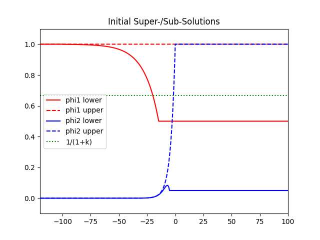
We consider the pairs of functions \((\overline{\phi}, \overline{\psi})\) and \((\underline{\phi}, \underline{\psi})\) respectively, to the system (1), where \[\begin{aligned} \overline{\phi}(t) &= \begin{cases} 1 – \varepsilon\left(e^{\lambda_1 t} – e^{\gamma \lambda_1 t}\right), & t < 0, \\ 1, & t \ge 0, \end{cases} & \underline{\phi}(t) &= \begin{cases} 1 – k, & t > t_1, \\ 1 – k\left(e^{\lambda_1 t} + p e^{\eta \lambda_1 t}\right), & t \le t_1, \end{cases} \\ \overline{\psi}(t) &= \begin{cases} 1, & t > 0, \\ e^{\lambda_2 t}, & t \le 0, \end{cases} & \underline{\psi}(t) &= \begin{cases} \sigma, & t > t_2, \\ e^{\lambda_2 t} – q e^{\kappa \lambda_2 t}, & t \le t_2. \end{cases} \end{aligned}\]
We assume the following conditions: \[\begin{aligned} \gamma &> \max\left\{1, \frac{\lambda_2}{\lambda_1}\right\}, \\ \kappa &\in \left(1, \min\left(\frac{\lambda_3}{\lambda_2}, 2\right)\right), \end{aligned}\] and that \(\eta > 0\) is sufficiently small so that \(\lambda_2 > \eta \lambda_1\) and
\[\begin{aligned} &\varepsilon < \min \left( \alpha_1k\sigma, \frac{\alpha_1k\left(1-qe^{\kappa – 1}e^{\lambda_2t_2}\right)}{\int_{-\infty}^{\infty}J_1(y)e^{-\gamma\lambda_1y}dy – e^{-\lambda_1\gamma r_1} – c\gamma\lambda_1 – \alpha_1 + \alpha_1k} \right)\\ &p > \frac{\alpha_1(k+1)}{-\left[\int_{\mathbb{R}} J_1(y)e^{-\eta\lambda_1(y+r_1)}dy – e^{-\eta\lambda_1r_1} – c\eta\lambda_1 – \alpha_1 + \alpha_1k\right]}\\ & \int_{\mathbb{R}} J_1(y)e^{-\eta\lambda_1(y+r_1)}dy – e^{-\eta\lambda_1r_1} – c\eta\lambda_1 – \alpha_1 + \alpha_1k < 0\\ &q > \max\left( 1, \frac{\alpha_2}{-(1-k)\left[\int_{\mathbb{R}}J_2(y)e^{-\kappa\lambda_2(y+r_3)}dy – e^{-\kappa\lambda_2r_3} – c\kappa\lambda_2 + \alpha_2\right]}\right). \end{aligned}\]
Lemma 5. Define \(\underline{\phi}(t), \underline{\psi}(t), \overline{\phi}(t), \overline{\psi}(t)\) as above, then the following hold
1. \(0\le \underline{\phi}(t)\le \overline{\phi}(t), \quad 0\le \underline{\psi}(t)\le \overline{\psi}(t).\)
2. \(\underline{\phi}'(t_1^-)\le \underline{\phi}'(t_1^+), \quad \overline{\phi}'(0^-)\ge \overline{\phi}'(0^+), \quad \underline{\psi}'(t_2^-)\le \underline{\psi}'(t_2^+), \quad \overline{\psi}'(0^-)\ge \overline{\psi}'(0^+).\)
3. \((\overline{\phi}(t), \overline{\psi}(t)), (\underline{\phi}(t), \underline{\psi}(t))\) is a pair of super/sub solutions for the system (1).
Proof. The proof for part \(i\) is obvious. Looking at part \(ii\) we see the following Table 1.
| Function | Transition point | Left derivative | Right derivative |
|---|---|---|---|
| \(\overline{\phi}(t)\) | \(t = 0\) | \(-\varepsilon \lambda_1 (1 – \gamma)\) | \(0\) |
| \(\underline{\phi}(t)\) | \(t = t_1\) | \(-k\left( \lambda_1 e^{\lambda_1 t_1} + p \eta \lambda_1 e^{\eta \lambda_1 t_1} \right)\) | \(0\) |
| \(\overline{\psi}(t)\) | \(t = 0\) | \(\lambda_2\) | \(0\) |
| \(\underline{\psi}(t)\) | \(t = t_2\) | \(\lambda_2 e^{\lambda_2 t_2} – q \kappa \lambda_1 e^{\kappa \lambda_1 t_2}\) | \(0\) |
Seeing \(\gamma>1\) the result is clear.
For part \(iii\) we see that the functions are continuously differentiable outside a finite number of points. To show the inequalities we proceed in cases.
Case 1. \(t > r_1\).
In this case, we have \(\overline{\phi}(t – r_1) = 1\), \(\overline{\phi}(t) = 1\), and \(0 \le \underline{\psi}(t – r_2) \le \sigma\). Then, \[\begin{aligned} \int_{-\infty}^{\infty} J_1(y) &\left[ \overline{\phi}(t – y – r_1) – \overline{\phi}(t – r_1) \right] dy – c \, \overline{\phi}'(t) + \alpha_1 \overline{\phi}(t) \left[ 1 – \overline{\phi}(t) – k \, \underline{\psi}(t – r_2) \right] \\ &= \int_{-\infty}^{\infty} J_1(y) \overline{\phi}(t – y – r_1) dy – \int_{-\infty}^{\infty} J_1(y) dy + \alpha_1 \cdot 1 \cdot \left[ 1 – 1 – k \, \underline{\psi}(t – r_2) \right] \\ &= \int_{-\infty}^{\infty} J_1(y) \overline{\phi}(t – y – r_1) dy – 1 – \alpha_1 k \, \underline{\psi}(t – r_2) \\ &\le -\alpha_1 k \, \underline{\psi}(t – r_2) \\ &\le 0. \end{aligned}\]
Case 2. \(0 \le t \le r_1\), \(t_2 < t – r_2\).
In this case, we have \[\overline{\phi}(t – r_1) = 1 – \varepsilon\left( e^{\lambda_1(t – r_1)} – e^{\gamma \lambda_1(t – r_1)} \right), \quad \overline{\phi}(t) = 1, \quad \underline{\psi}(t – r_2) = \sigma.\]
Then, \[\begin{aligned} \int_{-\infty}^{\infty} J_1(y) &\left[ \overline{\phi}(t – y – r_1) – \overline{\phi}(t – r_1) \right] dy – c \, \overline{\phi}'(t) + \alpha_1 \overline{\phi}(t) \left[ 1 – \overline{\phi}(t) – k \, \underline{\psi}(t – r_2) \right] \\ &= \int_{-\infty}^{\infty} J_1(y) \overline{\phi}(t – y – r_1) dy – \overline{\phi}(t – r_1) \int_{-\infty}^{\infty} J_1(y) dy – \alpha_1 k \sigma \\ &= \int_{-\infty}^{t – r_1} J_1(y) \overline{\phi}(t – y – r_1) dy + \int_{t – r_1}^{\infty} J_1(y) \overline{\phi}(t – y – r_1) dy – \overline{\phi}(t – r_1) – \alpha_1 k \sigma \\ &= \int_{-\infty}^{t – r_1} J_1(y) dy + \int_{t – r_1}^{\infty} J_1(y) \left[ 1 – \varepsilon \left( e^{\lambda_1(t – y – r_1)} – e^{\gamma \lambda_1(t – y – r_1)} \right) \right] dy \\ &\quad – \left[ 1 – \varepsilon \left( e^{\lambda_1(t – r_1)} – e^{\gamma \lambda_1(t – r_1)} \right) \right] – \alpha_1 k \sigma \\ &= \int_{-\infty}^{\infty} J_1(y) dy – \varepsilon \int_{t – r_1}^{\infty} J_1(y) \left( e^{\lambda_1(t – y – r_1)} – e^{\gamma \lambda_1(t – y – r_1)} \right) dy \\ &\quad – 1 + \varepsilon \left( e^{\lambda_1(t – r_1)} – e^{\gamma \lambda_1(t – r_1)} \right) – \alpha_1 k \sigma \\ &= – \varepsilon \int_{t – r_1}^{\infty} J_1(y) \left( e^{\lambda_1(t – y – r_1)} – e^{\gamma \lambda_1(t – y – r_1)} \right) dy \\ &\quad + \varepsilon \left( e^{\lambda_1(t – r_1)} – e^{\gamma \lambda_1(t – r_1)} \right) – \alpha_1 k \sigma. \end{aligned}\]
So, \[\begin{aligned} – \varepsilon \int_{t – r_1}^{\infty} J_1(y) &\left( e^{\lambda_1(t – y – r_1)} – e^{\gamma \lambda_1(t – y – r_1)} \right) dy + \varepsilon \left( e^{\lambda_1(t – r_1)} – e^{\gamma \lambda_1(t – r_1)} \right) – \alpha_1 k \sigma \\ &\le \varepsilon \left( e^{\lambda_1(t – r_1)} – e^{\gamma \lambda_1(t – r_1)} \right) – \alpha_1 k \sigma \\ &\le \varepsilon – \alpha_1 k \sigma. \end{aligned}\] Thus, the inequality is satisfied whenever \(\varepsilon \le \alpha_1 k \sigma\).
Case 3. \(t_2 – r_2 \le t \le 0\).
In this case, we have \(\underline{\psi}(t – r_2) = \sigma\). Then, \[\begin{aligned} \int_{-\infty}^{\infty} J_1(y) &\left[ \overline{\phi}(t – y – r_1) – \overline{\phi}(t – r_1) \right] dy – c \, \overline{\phi}'(t) + \alpha_1 \overline{\phi}(t) \left[ 1 – \overline{\phi}(t) – k \, \underline{\psi}(t – r_2) \right] \\ = \; &\int_{-\infty}^{t – r_1} J_1(y) dy + \int_{t – r_1}^{\infty} J_1(y) \left[ 1 – \varepsilon \left( e^{\lambda_1(t – y – r_1)} – e^{\gamma \lambda_1(t – y – r_1)} \right) \right] dy \\ &\quad – \left[ 1 – \varepsilon \left( e^{\lambda_1(t – r_1)} – e^{\gamma \lambda_1(t – r_1)} \right) \right] + c \varepsilon \left( \lambda_1 e^{\lambda_1 t} – \gamma \lambda_1 e^{\gamma \lambda_1 t} \right) \\ &\quad + \alpha_1 \left[ 1 – \varepsilon \left( e^{\lambda_1 t} – e^{\gamma \lambda_1 t} \right) \right] – \alpha_1 \left[ 1 – \varepsilon \left( e^{\lambda_1 t} – e^{\gamma \lambda_1 t} \right) \right]^2 – \alpha_1 k \sigma \left[ 1 – \varepsilon \left( e^{\lambda_1 t} – e^{\gamma \lambda_1 t} \right) \right] \\ = \; &\int_{-\infty}^{\infty} J_1(y) dy – 1 – \varepsilon \int_{t – r_1}^{\infty} J_1(y) \left( e^{\lambda_1(t – y – r_1)} – e^{\gamma \lambda_1(t – y – r_1)} \right) dy + \varepsilon \left( e^{\lambda_1 t} – e^{\gamma \lambda_1 t} \right) \\ &\quad + c \varepsilon \left( \lambda_1 e^{\lambda_1 t} – \gamma \lambda_1 e^{\gamma \lambda_1 t} \right) + \alpha_1 \varepsilon \left( e^{\lambda_1 t} – e^{\gamma \lambda_1 t} \right) – \alpha_1 \varepsilon^2 \left( e^{\lambda_1 t} – e^{\gamma \lambda_1 t} \right)^2 \\ &\quad – \alpha_1 k \sigma \left[ 1 – \varepsilon \left( e^{\lambda_1 t} – e^{\gamma \lambda_1 t} \right) \right] \\ = \; &\varepsilon e^{\lambda_1 t} \left[ – \int_{t – r_1}^{\infty} J_1(y) e^{- \lambda_1 (y + r_1)} dy + e^{- \lambda_1 r_1} + c \lambda_1 + \alpha_1 \right] \\ &\quad – \alpha_1 \varepsilon^2 \left( e^{\lambda_1 t} – e^{\gamma \lambda_1 t} \right)^2 \\ &\quad + \varepsilon e^{\gamma \lambda_1 t} \left[ \int_{t – r_1}^{\infty} J_1(y) e^{- \gamma \lambda_1 (y + r_1)} dy – e^{- \gamma \lambda_1 r_1} – c \gamma \lambda_1 – \alpha_1 \right] \\ &\quad – \alpha_1 k \sigma \left[ 1 – \varepsilon \left( e^{\lambda_1 t} – e^{\gamma \lambda_1 t} \right) \right] \\ < \; &\varepsilon e^{\lambda_1 t} \left[ – \int_{t – r_1}^{\infty} J_1(y) e^{- \lambda_1 (y + r_1)} dy + \int_{-\infty}^{\infty} J_1(y) e^{- \lambda_1 (y + r_1)} dy \right] – \alpha_1 k \sigma + \alpha_1 k \sigma \varepsilon e^{\lambda_1 t} \\ &\quad + \varepsilon e^{\gamma \lambda_1 t} \left[ \int_{-\infty}^{\infty} J_1(y) e^{- \gamma \lambda_1 (y + r_1)} dy – e^{- \gamma \lambda_1 r_1} – c \gamma \lambda_1 – \alpha_1 \right] \\ &\quad + \varepsilon e^{\gamma \lambda_1 t} \int_{-\infty}^{t – r_1} J_1(y) e^{- \gamma \lambda_1 (y + r_1)} dy \\ = \; &\varepsilon \int_{0}^{\infty} J_1(t – x – r_1) \left[ e^{\lambda_1(x – r_1)} – e^{\gamma \lambda_1(x – r_1)} \right] dx \\ &\quad + \varepsilon e^{\gamma \lambda_1 t} \left[ \int_{-\infty}^{\infty} J_1(y) e^{- \gamma \lambda_1 (y + r_1)} dy – e^{- \gamma \lambda_1 r_1} – c \gamma \lambda_1 – \alpha_1 \right] \\ &\quad + \alpha_1 k \sigma \varepsilon e^{\lambda_1 t} – \alpha_1 k \sigma \\ < \; &\varepsilon \left[ \int_{-\infty}^{\infty} J_1(y) e^{- \gamma \lambda_1 y} dy – e^{- \gamma \lambda_1 r_1} – c \gamma \lambda_1 – \alpha_1 + \alpha_1 k \sigma \right] – \alpha_1 k \sigma < \; 0. \end{aligned}\]
Case 4. \(t < t_2 + r_2\).
In this case, we have \[\underline{\psi}(t – r_2) = e^{\lambda_2 t} – q e^{\kappa \lambda_2 t}.\]
Then, \[\begin{aligned} \int_{-\infty}^{\infty} J_1(y) &\overline{\phi}(t – y – r_1) dy – \overline{\phi}(t – r_1) – c \, \overline{\phi}'(t) + \alpha_1 \overline{\phi}(t) \left[ 1 – \overline{\phi}(t) – k \, \underline{\psi}(t – r_2) \right] \\ =\; &\int_{-\infty}^{t – r_1} J_1(y) dy + \int_{t – r_1}^{\infty} J_1(y) \left[ 1 – \varepsilon \left( e^{\lambda_1(t – y – r_1)} – e^{\gamma \lambda_1(t – y – r_1)} \right) \right] dy \\ &\quad – \left[ 1 – \varepsilon \left( e^{\lambda_1(t – r_1)} – e^{\gamma \lambda_1(t – r_1)} \right) \right] + c \varepsilon \left( \lambda_1 e^{\lambda_1 t} – \gamma \lambda_1 e^{\gamma \lambda_1 t} \right) \\ &\quad + \alpha_1 \left[ 1 – \varepsilon \left( e^{\lambda_1(t – r_1)} – e^{\gamma \lambda_1(t – r_1)} \right) \right] \left[ \varepsilon \left( e^{\lambda_1 t} – e^{\gamma \lambda_1 t} \right) – k \left( e^{\lambda_2(t – r_2)} – q e^{\kappa \lambda_2(t – r_2)} \right) \right] \\ <\; &\varepsilon \int_0^{\infty} J_1(t – x – r_1) \left( e^{\lambda_1(x – r_1)} – e^{\gamma \lambda_1(x – r_1)} \right) dx \\ &\quad + \varepsilon e^{\gamma \lambda_1 t} \left[ \int_{-\infty}^{\infty} J_1(y) e^{- \gamma \lambda_1 (y + r_1)} dy – e^{- \gamma \lambda_1 r_1} – c \gamma \lambda_1 – \alpha_1 \right] \\ &\quad + \alpha_1 k \varepsilon \left( e^{\lambda_1 t} – e^{\gamma \lambda_1 t} \right) \left( e^{\lambda_2 t} – q e^{\kappa \lambda_2 t} \right) – \alpha_1 k \left( e^{\lambda_2 t} – q e^{\kappa \lambda_2 t} \right) \\ <\; &e^{\lambda_2 t} \left\{ \varepsilon \left[ \int_{-\infty}^{\infty} J_1(y) e^{- \gamma \lambda_1 y} dy – e^{- \gamma \lambda_1 r_1} – c \gamma \lambda_1 – \alpha_1 + \alpha_1 k \right] – \alpha_1 k \left( 1 – q e^{(\kappa – 1)} e^{\lambda_2 t_2} \right) \right\} <\; 0. \end{aligned}\]
Case 1. \(t > t_1 + r_1\).
In this case, \(\underline{\phi}(t) = 1 – k\). Then, \[\begin{aligned} \int_{\mathbb{R}} J_1(y) &\left[ \underline{\phi}(t – y – r_1) – \underline{\phi}(t – r_1) \right] dy – c \, \underline{\phi}'(t) + \alpha_1 \underline{\phi}(t) \left[ 1 – \underline{\phi}(t) – k \overline{\psi}(t – r_2) \right] \\ \ge\; &\int_{\mathbb{R}} J_1(y)(1 – k) dy – (1 – k) + \alpha_1 (1 – k) \left[ 1 – (1 – k) – k \overline{\psi}(t – r_2) \right] \\ =\; &(1 – k) \int_{\mathbb{R}} J_1(y) dy – (1 – k) + \alpha_1 k (1 – k) \left[ 1 – \overline{\psi}(t – r_2) \right] \\ =\; &\alpha_1 k (1 – k) \left[ 1 – \overline{\psi}(t – r_2) \right] \ge\; 0. \end{aligned}\]
Case 2. \(t_1 < t \le t_1 + r_1\).
Here, \[\underline{\phi}(t – r_1) = 1 – k \left( e^{\lambda_1 t} + p e^{\eta \lambda_1 t} \right), \quad \underline{\phi}(t) = 1 – k.\]
Then, \[\begin{aligned} \int_{\mathbb{R}} J_1(y) &\left[ \underline{\phi}(t – y – r_1) – \underline{\phi}(t – r_1) \right] dy – c \, \underline{\phi}'(t) + \alpha_1 \underline{\phi}(t) \left[ 1 – \underline{\phi}(t) – k \overline{\psi}(t – r_2) \right] \\ =\; &\int_{\mathbb{R}} J_1(y) \left[ \underline{\phi}(t – y – r_1) \right] dy – \underline{\phi}(t – r_1) + \alpha_1 k (1 – k) \left[ 1 – \overline{\psi}(t – r_2) \right] \\ =\; &\int_{\mathbb{R}} J_1(y) \left[ 1 – k \left( e^{\lambda_1(t – y – r_1)} + p e^{\eta \lambda_1(t – y – r_1)} \right) \right] dy – \left[ 1 – k \left( e^{\lambda_1(t – r_1)} + p e^{\eta \lambda_1(t – r_1)} \right) \right] \\ &\quad + \alpha_1 k (1 – k) \left[ 1 – \overline{\psi}(t – r_2) \right] \\ =\; &-k \left[ \int_{\mathbb{R}} J_1(y) \left( e^{\lambda_1(t – y – r_1)} + p e^{\eta \lambda_1(t – y – r_1)} \right) dy – e^{\lambda_1(t – r_1)} – p e^{\eta \lambda_1(t – r_1)} \right] \\ &\quad + \alpha_1 k (1 – k) \left[ 1 – \overline{\psi}(t – r_2) \right] \ge\; 0. \end{aligned}\]
Case 3. \(t \le t_1\).
In this case, \[\underline{\phi}(t) = 1 – k\left( e^{\lambda_1 t} + p e^{\eta \lambda_1 t} \right), \quad \overline{\psi}(t) = e^{\lambda_2 t}.\]
Then, \[\begin{aligned} \int_{\mathbb{R}} J_1(y) &\left[ \underline{\phi}(t – y – r_1) – \underline{\phi}(t – r_1) \right] dy – c \, \underline{\phi}'(t) + \alpha_1 \underline{\phi}(t) \left[ 1 – \underline{\phi}(t) – k \, \overline{\psi}(t – r_2) \right] \\ \ge\; &\int_{\mathbb{R}} J_1(y) \left[ 1 – k \left( e^{\lambda_1(t – y – r_1)} + p e^{\eta \lambda_1(t – y – r_1)} \right) \right] dy – \left[ 1 – k \left( e^{\lambda_1(t – r_1)} + p e^{\eta \lambda_1(t – r_1)} \right) \right] \\ &\quad + c k \left( \lambda_1 e^{\lambda_1 t} + p \eta \lambda_1 e^{\eta \lambda_1 t} \right) + \alpha_1 k \left( e^{\lambda_1 t} + p e^{\eta \lambda_1 t} \right) – \alpha_1 k^2 \left( e^{\lambda_1 t} + p e^{\eta \lambda_1 t} \right)^2 \\ &\quad – \alpha_1 k e^{\lambda_2(t – r_2)} + \alpha_1 k \left( e^{\lambda_1 t} + p e^{\eta \lambda_1 t} \right) e^{\lambda_2(t – r_2)} \\ \ge\; &-k \int_{\mathbb{R}} J_1(y) \left( e^{\lambda_1(t – y – r_1)} + p e^{\eta \lambda_1(t – y – r_1)} \right) dy + k \left( e^{\lambda_1(t – r_1)} + p e^{\eta \lambda_1(t – r_1)} \right) \\ &\quad + c k \left( \lambda_1 e^{\lambda_1 t} + p \eta \lambda_1 e^{\eta \lambda_1 t} \right) + \alpha_1 k \left( e^{\lambda_1 t} + p e^{\eta \lambda_1 t} \right) – \alpha_1 k^2 \left( e^{\lambda_1 t} + p e^{\eta \lambda_1 t} \right)^2 \\ &\quad – \alpha_1 k e^{\lambda_2(t – r_2)} + \alpha_1 k \left( e^{\lambda_1 t} + p e^{\eta \lambda_1 t} \right) e^{\lambda_2(t – r_2)} \\ =\; &k e^{\lambda_1 t} \left[ – \int_{\mathbb{R}} J_1(y) e^{-\lambda_1(y + r_1)} dy + e^{-\lambda_1 r_1} + c \lambda_1 – \alpha_1 \right] \\ &\quad + k e^{\eta \lambda_1 t} \left[ p \left( – \int_{\mathbb{R}} J_1(y) e^{-\eta \lambda_1(y + r_1)} dy + e^{-\eta \lambda_1 r_1} + c \eta \lambda_1 \right) + \alpha_1(k – 1) \right] \\ &\quad – r k e^{(1 – \eta)\lambda_1 t} – r e^{(\lambda_2 – \eta \lambda_1)(t – r_1)} \\ \ge\; &k e^{\eta \lambda_1 t} \left[ -p \left( \int_{\mathbb{R}} J_1(y) e^{-\eta \lambda_1(y + r_1)} dy – e^{-\eta \lambda_1 r_1} – c \eta \lambda_1 \right) – \alpha_1(k + 1) \right] >\; 0. \end{aligned}\]
Case 1. \(t > r_3\).
We assume \(r_4 < r_3\), so \(\overline{\psi}(t) = 1\) and \(\overline{\phi}(t – r_4) = \overline{\phi}(t) = 1\). Then, \[\begin{aligned} \int_{\mathbb{R}} J_2(y) &\left[ \overline{\psi}(t – y – r_3) – \overline{\psi}(t – r_3) \right] dy – c \, \overline{\psi}'(t) + \alpha_2 \overline{\psi}(t) \left[ 1 – \frac{\overline{\psi}(t)}{\overline{\phi}(t – r_4)} \right] \\ =\; &\int_{\mathbb{R}} J_2(y) \overline{\psi}(t – y – r_3) dy – \overline{\psi}(t – r_3) \\ =\; &\int_{\mathbb{R}} J_2(y) \overline{\psi}(t – y – r_3) dy – 1 \le\; 0. \end{aligned}\]
Case 2. \(0 < t < r_3\).
In this case, we have \(\overline{\psi}(t) = 1\), \(\overline{\phi}(t) = 1\), \(\overline{\phi}(t – r_4) \le 1\), and \(\overline{\psi}(t – r_3) = e^{\lambda_2(t – r_3)}\). Then, \[\begin{aligned} \int_{\mathbb{R}} J_2(y) &\left[ \overline{\psi}(t – y – r_3) – \overline{\psi}(t – r_3) \right] dy – c \, \overline{\psi}'(t) + \alpha_2 \overline{\psi}(t) \left[ 1 – \frac{\overline{\psi}(t)}{\overline{\phi}(t – r_4)} \right] \\ \le\; &\int_{\mathbb{R}} J_2(y) \left[ \overline{\psi}(t – y – r_3) – \overline{\psi}(t – r_3) \right] dy + \alpha_2 \left[ 1 – \overline{\psi}(t) \right] \\ =\; &\int_{\mathbb{R}} J_2(y) \overline{\psi}(t – y – r_3) dy – \overline{\psi}(t – r_3) \\ =\; &\int_{\mathbb{R}} J_2(y) e^{\lambda_2(t – y – r_3)} dy – e^{\lambda_2(t – r_3)} \\ =\; &e^{\lambda_2(t – r_3)} \left[ \int_{\mathbb{R}} J_2(y) e^{-\lambda_2 y} dy – 1 \right] \le\; 0. \end{aligned}\]
Case 3. \(t < 0\).
Then, \[\begin{aligned} \int_{\mathbb{R}} J_2(y) &\left[ \overline{\psi}(t – y – r_3) – \overline{\psi}(t – r_3) \right] dy – c \, \overline{\psi}'(t) + \alpha_2 \overline{\psi}(t) \left[ 1 – \frac{\overline{\psi}(t)}{\overline{\phi}(t – r_4)} \right] \\ =\; &\int_{\mathbb{R}} J_2(y) e^{\lambda_2(t – y – r_3)} dy – e^{\lambda_2(t – r_3)} – c \lambda_2 e^{\lambda_2 t} + \alpha_2 e^{\lambda_2 t} – \alpha_2 \frac{\overline{\psi}^2(t)}{\overline{\phi}(t – r_4)} \\ =\; &e^{\lambda_2 t} \left[ \int_{\mathbb{R}} J_2(y) e^{-\lambda_2(y + r_3)} dy – e^{-\lambda_2 r_3} – c \lambda_2 + \alpha_2 \right] – \alpha_2 \frac{\overline{\psi}^2(t)}{\overline{\phi}(t – r_4)} \\ =\; &- \alpha_2 \frac{\overline{\psi}^2(t)}{\overline{\phi}(t – r_4)} <\; 0. \end{aligned}\]
We define \[\mathcal{M}(t) = e^{\lambda_2 t} – q e^{\kappa \lambda_2 t}, \quad \mathcal{N}(t) = \int_{-\infty}^{t} J_2(y – x) \mathcal{M}(x) \, dx – \frac{\mathcal{M}(t)}{2}.\]
Note that \(\mathcal{M}(t) > 0\) on \((-\infty, t_0)\), where \(t_0 = \frac{-\ln(q)}{(\kappa – 1)\lambda_2}\) is the unique root of \(\mathcal{M}\). Let \(\mathcal{M}(t_m)\) be the unique maximum of \(\mathcal{M}\). Then there exists a sufficiently small value \(\sigma \in (0, 1 – k)\) and a corresponding \(t_2 \in (t_m, t_0)\) such that \[\begin{aligned} \mathcal{M}(t_2) &= \sigma, \\ \mathcal{N}(t_2) &\ge 0. \end{aligned}\]
Case 1. \(t > t_2 + r_3\).
In this case, we have \(\underline{\phi}(t – r_4) \ge 1 – k\) and \(\underline{\psi}(t) = \underline{\psi}(t – r_3) = \sigma\). Then, \[\begin{aligned} \int_{\mathbb{R}} J_2(y) &\left[ \underline{\psi}(t – y – r_3) – \underline{\psi}(t – r_3) \right] dy – c \, \underline{\psi}'(t) + \alpha_2 \underline{\psi}(t) \left[ 1 – \frac{\underline{\psi}(t)}{\underline{\phi}(t – r_4)} \right] \\ \ge\; &\int_{\mathbb{R}} J_2(y) \underline{\psi}(t – y – r_3) \, dy – \underline{\psi}(t – r_3) + \alpha_2 \sigma \left[ 1 – \frac{\sigma}{1 – k} \right] \\ =\; &\int_{\mathbb{R}} J_2(y) \underline{\psi}(t – y – r_3) \, dy – \sigma + \alpha_2 \sigma \left[ 1 – \frac{\sigma}{1 – k} \right] \\ =\; &\int_{t – (t_2 – r_3)}^{\infty} J_2(y) \left( e^{\lambda_2(t – y – r_3)} – q e^{\kappa \lambda_2(t – y – r_3)} \right) dy \\ &\quad + \int_{-\infty}^{t – (t_2 – r_3)} J_2(y) \sigma \, dy – \sigma + \alpha_2 \sigma \left[ 1 – \frac{\sigma}{1 – k} \right] \\ \ge\; &\int_{-\infty}^{t_2 – r_3} J_2(t – (y – r_3)) \left( e^{\lambda_2(y – r_3)} – q e^{\kappa \lambda_2(y – r_3)} \right) dy + \frac{\sigma}{2} – \sigma + \alpha_2 \sigma \left[ 1 – \frac{\sigma}{1 – k} \right] \\ \ge\; &\frac{\mathcal{M}(t_2)}{2} – \frac{\sigma}{2} + \alpha_2 \sigma \left[ 1 – \frac{\sigma}{1 – k} \right] \\ =\; &\alpha_2 \sigma \left[ 1 – \frac{\sigma}{1 – k} \right] >\; 0. \end{aligned}\]
Case 2. \(t_2 < t \le t_2 + r_3\).
In this case, \[\underline{\psi}(t) = \sigma > \underline{\psi}(t – r_3) = e^{\lambda_2(t – r_3)} – q e^{\kappa \lambda_2(t – r_3)}, \quad \underline{\phi}(t – r_4) \ge 1 – k.\]
Then, \[\begin{aligned} \int_{\mathbb{R}} J_2(y) &\left[ \underline{\psi}(t – y – r_3) – \underline{\psi}(t – r_3) \right] dy – c \, \underline{\psi}'(t) + \alpha_2 \underline{\psi}(t) \left[ 1 – \frac{\underline{\psi}(t)}{\underline{\phi}(t – r_4)} \right] \\ \ge\; &\int_{\mathbb{R}} J_2(y) \underline{\psi}(t – y – r_3) \, dy – \underline{\psi}(t – r_3) + \alpha_2 \sigma \left[ 1 – \frac{\sigma}{1 – k} \right] \\ \ge\; &\int_{\mathbb{R}} J_2(y) \underline{\psi}(t – y – r_3) \, dy – \sigma + \alpha_2 \sigma \left[ 1 – \frac{\sigma}{1 – k} \right] \\ \ge\; &\frac{\mathcal{M}(t_2)}{2} – \frac{\sigma}{2} + \alpha_2 \sigma \left[ 1 – \frac{\sigma}{1 – k} \right] \\ =\; &\alpha_2 \sigma \left[ 1 – \frac{\sigma}{1 – k} \right] >\; 0. \end{aligned}\]
Case 3. \(t \le t_2\).
Then, \[\begin{aligned} &\int_{\mathbb{R}}J_2(y)\left[\underline{\psi}(t-y-r_3) – \underline{\psi}(t-r_3)\right] – c\underline{\psi}'(t) + \alpha_2\underline{\psi}(t)\left[1 – \frac{\underline{\psi}(t)}{\underline{\phi}(t-r_4)}\right] \\ &\qquad\ge \int_{\mathbb{R}}J_2(y)\underline{\psi}(t-y-r_3)dy – \underline{\psi}(t-r_3) -c\underline{\psi}'(t) + \alpha_2\underline{\psi}(t)\left[1 – \frac{\underline{\psi}(t)}{1-k}\right] \\ &\qquad\ge \int_{-\infty}^{\infty}J_2(y)\left(e^{\lambda_2(t-y-r_3)} – qe^{\kappa\lambda_2(t-y-r_3)}\right)dy – \left(e^{\lambda_2(t-r_3)} – qe^{\kappa\lambda_2(t-r_3)}\right) \\ &\qquad\quad- c\left(\lambda_2e^{\lambda_2t} – \kappa\lambda_2qe^{\kappa\lambda_2t}\right) + \alpha_2\left(e^{\lambda_2t} – qe^{\kappa\lambda_2t}\right) – \frac{\alpha_2}{1-k}\left(e^{\lambda_2t} – qe^{\kappa\lambda_2t}\right)^2 \\ &\qquad\ge e^{\lambda_2t}\left[\int_{\mathbb{R}}J_2(y)e^{-\lambda_2(y+r_3)}dy – e^{-\lambda_2r_3} – c\lambda_2 + \alpha_2\right] \\ &\qquad\quad+ e^{\kappa\lambda_2t}\left[-q\left[\int_{\mathbb{R}}J_2(y)e^{-\kappa\lambda_2(y+r_3)}dy – e^{-\kappa\lambda_2r_3} – c\kappa\lambda_2 + \alpha_2\right] – \frac{\alpha_2}{1-k}\right] \\ &\qquad> 0. \end{aligned}\] ◻
Corollary 3. Define \(\underline{\phi}(t), \underline{\psi}(t), \overline{\phi}(t), \overline{\psi}(t)\) as above, then \(\mathcal{T}\left((\underline{\phi}(t), \underline{\psi}(t)), (\overline{\phi}(t), \overline{\psi}(t))\right)\) is a lower/upper solution.
Lemma 6. Let \(\phi_1\) and \(\phi_2\) be the solutions of of the wave system in \(\Gamma\) defined above, then \[\lim_{t\to \infty}\left(\phi_1,\phi_2\right)(t)=\left(\frac{1}{1+k},\frac{1}{1+k}\right).\]
Proof. Define the truncated continuous functions \[f(\theta)=\begin{cases} &\frac{\theta}{1+k}, \quad \theta\in [0,1]\\ &0, \quad \theta \in [-r,0) \end{cases}, \quad g(\theta)=\begin{cases} &\frac{\theta}{1+k}(1-\theta)(1+\varepsilon), \quad \theta\in [0,1]\\ &1+\varepsilon, \quad \theta \in [-r,0). \end{cases}\]
Moreover, \(f'(0^-)=0<f'(0^+), g'(0^-)=0>g'(0^+)\) and \(f'(\theta)>0, g'(\theta)<0\) for \(\theta\in [0,1]\) provided \(\varepsilon>0\) is small enough such that \(k(1+\varepsilon)<1.\) Now, we notice \[\begin{aligned} &\liminf_{t\to \infty} \phi_1(t)\ge 1-k>0, \quad\liminf_{t\to \infty} \phi_2(t)\ge \sigma>0\\ &\limsup_{t\to \infty} \phi_1(t)\le 1, \quad\liminf_{t\to \infty} \phi_2(t)\le 1. \end{aligned}\]
Now, denoting \[\phi_i^-=\liminf_{t\to \infty} \phi_i, \quad \phi_i^+=\limsup_{t\to \infty} \phi_i, i=1,2.\]
It is easy to see for any \(-\tilde{r}\in [r,0]\) and the definition of the super/sub solutions \[f(-\tilde{r})=f(0)=0<\phi_i^-\le \phi_i^+<1+\varepsilon=g(0)=g(-\tilde{r}).\]
Thus, the result with delay present follows in the same manner as the non delay case. Let us define
\(\tilde{\theta}=\sup \left\{\theta\in [0,1) \quad | \quad f(\theta)<\phi_i^-\le \phi_i^+<g(\theta) \right\}.\) We claim that \(\tilde{\theta}=1\) and \[f( \tilde{\theta})=\phi_i^-= \phi_i^+=g( \tilde{\theta}).\] The proof is similar to that for theorem 2.6 in [1]. The proof will be replicated for the readers convenience.
First, we assume \(\phi_1^+ = f(\tilde{\theta})\). If \(\phi_1\) is eventually monotone, then by the boundedness of \(\phi_1\) on \(\mathbb{R}\), we have \(\phi_1(+\infty)\) exists, and \[\label{int1} \int_0^{+\infty} \phi_1'(t) \, dt = \phi_1(+\infty) – \phi_1(0). \tag{5}\]
By the above equation (5), we have either \(\liminf_{t \to +\infty} \phi_1'(t) = 0\) if \(\phi_1'(t) \ge 0\) for \(t \gg 1\), or \(\limsup_{t \to +\infty} \phi_1'(t) = 0\) if \(\phi_1'(t) \le 0\) for \(t \gg 1\). Then we can choose a sequence \(\{x_n\}\) with \(x_n \to +\infty\) such that \(\lim_{n \to \infty} \phi_1(x_n) = f(\tilde{\theta})\), \(\lim_{n \to \infty} \phi_1'(x_n) = 0\). It is obvious that \(\limsup_{n \to \infty} \phi_2(x_n) \le g(\tilde{\theta})\). Then we get \[\begin{aligned} \liminf_{n \to \infty} [1 – \phi_1(x_n) – k d \phi_2(x_n)] &\ge 1 – f(\tilde{\theta}) – k g(\tilde{\theta}) \\ &= (1 – \tilde{\theta})[1 – k(1 + \varepsilon)] > 0. \end{aligned}\]
Integrating the \(\phi_1\)-equation of (1) from 0 to \(x_n\), we have \[\begin{aligned} \int_0^{x_n} c \phi_1'(t) \, dt &= \int_0^{x_n} \int_{\mathbb{R}} J_1(y) \phi_1(t – y-r_1) \, dy \, dt + \int_0^{x_n} \phi_1(t-r_1) \, dt \nonumber \\ &= \alpha_1 \int_0^{x_n} \phi_1(t) \left[ 1 – \phi_1(t) – k d \phi_2(t-r_2) \right] dt. \label{int2} \end{aligned} \tag{6}\]
Some simple calculations yield: \[\begin{aligned} – \int_0^{x_n} &\int_{\mathbb{R}} J_1(y) \phi_1(t – y-r_1) \, dy \, dt + \int_0^{x_n} \phi_1(t-r_1) \, dt\notag\\ &=\; \int_0^{x_n} \int_{\mathbb{R}} J_1(y) \left[ \phi_1(t-r_1) – \phi_1(t – y-r_1) \right] dy \, dt\nonumber \\ &=\; \int_{\mathbb{R}} J_1(y) \left[ \int_0^{x_n} \left( \phi_1(t-r_1) – \phi_1(t – y-r_1) \right) dt \right] dy \nonumber\\ &=\; \int_{\mathbb{R}} J_1(y) \left[ \int_0^{x_n} \int_0^y \phi_1'(t-r_1 + \eta y) \, d\eta \, dt \right] dy\nonumber \\ &=\; \int_{\mathbb{R}} J_1(y) \left[ \int_0^1 \int_0^{x_n} \phi_1'(t-r_1 + \eta y) \, dt \, d\eta \right] dy \nonumber\\ &=\; \int_{\mathbb{R}} J_1(y) \left[ \int_0^1 \left( \phi_1(x_n -r_1 + \eta y) – \phi_1(\eta y-r_1) \right) d\eta \right] dy \nonumber \\ &=\; \int_{\mathbb{R}} J_1(y) y \left[ \int_{-1}^{0} \phi_1(x_n-r_1 + \eta y) – \phi_1(\eta y-r_1) \, d\eta \right] dy.\label{int3} \end{aligned} \tag{7}\]
Let \(n \to \infty\) in (7). Then by using properties of \(J\), we have \[\begin{aligned} \int_{\mathbb{R}} J_1(y) y \left[ \int_{-1}^{0} f(\tilde{\theta}) – \phi_1(\eta y-r_1) \, d\eta \right] dy &= f(\tilde{\theta}) \int_{\mathbb{R}} J_1(y) y \, dy – \int_{\mathbb{R}} J_1(y) y \left[ \int_{-1}^{0} \phi_1(\eta y-r_1) \, d\eta \right] dy\nonumber \\ &= – \int_{\mathbb{R}} J_1(y) y \left[ \int_{-1}^{0} \phi_1(\eta y-r_1) \, d\eta \right] dy \nonumber \\ &\le \int_{\mathbb{R}} J_1(y) |y| \, d y = 2 \int_{0}^{\infty} J_1(y) y \, dy \nonumber\\ &\le 2 \int_{0}^{\infty} J_1(y) y e^{y} \, dy \le 2 \int_{\mathbb{R}} J_1(y) y e^{|y|} \, dy < \infty\label{int4}. \end{aligned} \tag{8}\]
Moreover, \(\lim_{n \to \infty} \int_0^{x_n} c \phi_1'(t) \, dt = \lim_{n \to \infty} c(\phi_1(x_n) – \phi_1(0)) = c(f(\tilde{\theta}) – \phi_1(0))\). Hence, the left-hand side of (7) is bounded, which is a contradiction since the right-hand side of (7) is unbounded. Hence \(f(\tilde{\theta}) = \phi_1^-\) is impossible. Therefore, \(f(\tilde{\theta}) < \phi_1^-\).
If \(\phi_1\) is oscillatory at \(\infty\), then we can choose a sequence \(\{x_n\}\) of minimal points of \(\phi_1\) with \(x_n \to \infty\) such that \[\lim_{n \to \infty} \phi_1(x_n) = f(\tilde{\theta}).\]
By the same argument as above, we also reach a contradiction. Hence \(f(\tilde{\theta}) < \phi_1^-\).
The impossibility for \(\phi_1^+ = g(\tilde{\theta})\) can be treated similarly, and we further get that \(\phi_1^+ < g(\tilde{\theta})\).
Next, we deal with the case \(\phi_2^- = f(\tilde{\theta})\). If \(\phi_2\) is eventually monotone, we have \(\phi_2(\infty)\) exists due to \(\phi_2\) being bounded on \(\mathbb{R}\). By a similar argument as the case \(\phi_1(\infty)\) exists, we can find a sequence \(\{x_n\}\) with \(x_n \to \infty\) such that \[\lim_{n \to \infty} \phi_2(x_n) = f(\tilde{\theta}) \quad \text{and} \quad \lim_{n \to \infty} \phi_2'(x_n) = 0.\]
Note that \[f(\tilde{\theta}) < \phi_1^- \le \phi_1^+ \le g(\tilde{\theta}),\] so
\[\begin{aligned} \label{inf1} \liminf_{n \to \infty} \left[1 – \frac{\phi_2(x_n)}{\phi_1(x_n-r_4)}\right] > 1 – \frac{f(\tilde{\theta})}{f(\tilde{\theta})} = 0. \end{aligned} \tag{9}\]
Integrating the \(\phi_2\)-equation of (1) from 0 to \(x_n\), we get \[\begin{aligned} \int_0^{x_n} c \phi_2'(t) \, dt &= \int_0^{x_n} \int_{\mathbb{R}} J_2(y) \phi_2(t – y-r_3) \, dy \, dt + \int_0^{x_n} \phi_2(t-r_2) \, dt \\ &= \alpha_2 \int_0^{x_n} \phi_2(t) \left[ 1 – \frac{\phi_2(t)}{\phi_1(t-r_4)} \right] dt. \end{aligned}\]
Let \(n \to \infty\), by a similar argument as (7), (8), and connecting (9), we obtain a contradiction.
On the other hand, if \(\phi_2\) is oscillatory at \(\infty\), then we can choose a sequence \(\{y_n\}\) of minimal points of \(\phi_2\) with \(y_n \to \infty\) such that \[\lim_{n \to \infty} \phi_2(y_n) = f(\tilde{\theta}).\]
Also, we have \[\liminf_{n \to \infty} \left[1 – \frac{\phi_2(y_n)}{\phi_1(y_n-r_4)}\right] > 1 – \frac{f(\tilde{\theta})}{f(\tilde{\theta})} = 0.\]
In this case, we still get a contradiction. Hence \(f(\tilde{\theta}) = \phi_2^-\) cannot occur. That is, \(f(\tilde{\theta}) < \phi_2^-\).
The impossibility for \(\phi_2^+ = g(\tilde{\theta})\) can be handled similarly, and we get that there holds \(\phi_2^+ < g(\tilde{\theta})\).
Therefore, \(\tilde{\theta} = 1\). So \(\frac{1}{1 + k} = f(1) \le \phi_1^+ \le \phi_1^- \le g(1) = \frac{1}{1 + k}\), hence \[(\phi_1, \phi_2)(+\infty) = \left( \frac{1}{1 + k}, \frac{1}{1 + k} \right).\] ◻
In this section, we present some numerical simulations. We discretize the traveling wave coordinate \(\xi = x – ct\) on a uniform mesh: \[\xi_j = \xi_{\min} + jh, \quad j = 0, 1, \dots, N,\] where \(h > 0\) is the mesh size and the domain is extended to the left by a buffer \(\delta_{\text{left}}\), so that \(\xi_{\min} = \xi_{\min}^{\text{phys}} – \delta_{\text{left}}\). The number of points \(N\) is chosen to ensure coverage of the desired interval.
The nonlocal diffusion is modeled using a truncated Gaussian kernel: \[J(y) = \frac{1}{\sqrt{\pi}} e^{-y^2}, \quad y \in [-M, M],\] discretized as \[\omega_i = \frac{1}{\sqrt{\pi}} e^{-(ih)^2}, \quad i = -i_M, \dots, i_M,\] with \(i_M = \lfloor M / h \rfloor\). For a function \(\phi\), the convolution \(\int_{\mathbb{R}} J(y)\, \phi(\xi – c\tau – y)\, dy,\) is approximated by \[\sum_{i = -i_M}^{i_M} \omega_i\, \phi_{j – s – i} \cdot h,\] where \(s = \lfloor c\tau / h \rfloor\) corresponds to the spatial shift induced by the delay \(\tau\).
The delayed nonlinear terms are defined pointwise as \[\begin{aligned} F_1[\phi_1, \phi_2]_j &= \alpha_1\, \phi_{1,j} \left(1 – \phi_{1,j} – k\, \phi_{2,j – s} \right) + \beta_1\, \phi_{1,j}, \\ F_2[\phi_1, \phi_2]_j &= \alpha_2\, \phi_{2,j} \left(1 – \frac{\phi_{2,j}}{\max(\phi_{1,j – s}, \varepsilon)} \right) + \beta_2\, \phi_{2,j}, \end{aligned}\] where \(\varepsilon > 0\) is a small parameter to avoid division by zero.
The numerical operators \(\mathcal{T}_1\) and \(\mathcal{T}_2\) are defined via left-sided quadrature: \[\begin{aligned} \mathcal{T}_1[\phi_1, \phi_2]_j &= \frac{1}{c} e^{-\frac{\gamma_1}{c} \xi_j} \sum_{i = 0}^{j} e^{\frac{\gamma_1}{c} \xi_i} \left( \mathrm{Diff}_{1,i} + F_1[\phi_1, \phi_2]_i \right) h, \\ \mathcal{T}_2[\phi_1, \phi_2]_j &= \frac{1}{c} e^{-\frac{\gamma_2}{c} \xi_j} \sum_{i = 0}^{j} e^{\frac{\gamma_2}{c} \xi_i} \left( \mathrm{Diff}_{2,i} + F_2[\phi_1, \phi_2]_i \right) h, \end{aligned}\] where the discrete diffusion contributions are given by \[\begin{aligned} \mathrm{Diff}_{1,i} &= \left( \sum_{m = -i_M}^{i_M} \omega_m\, \phi_{1,i – s – m} \right) h – \phi_{1,i – s}, \\ \mathrm{Diff}_{2,i} &= \left( \sum_{m = -i_M}^{i_M} \omega_m\, \phi_{2,i – s – m} \right) h – \phi_{2,i – s}. \end{aligned}\]
The following table gives the parameters.
| Parameter | Value |
|---|---|
| Wave speed and delay | |
| \(c\) | 4.0 |
| \(\tau_1 = \tau_2 = \tau_3 = \tau_4\) | 0.1 |
| Specific conditions | |
| \(\alpha_1 = \alpha_2\) | 1.0 |
| \(k\) | 0.5 |
| Super-/Sub-solution parameters | |
| \(\kappa\) | 2.0 |
| \(\lambda_1 = \lambda_2\) | 0.253961808106616 |
| \(\eta\) | 0.3 |
| \(\gamma\) | 2 |
| \(p = q\) | 3 |
| \(\varepsilon\) | 0.001 |
| \(\sigma\) | 0.05 |
| Operator parameters | |
| \({\beta_1}\) | 1.5913 |
| \({\beta_2}\) | 3.39 |
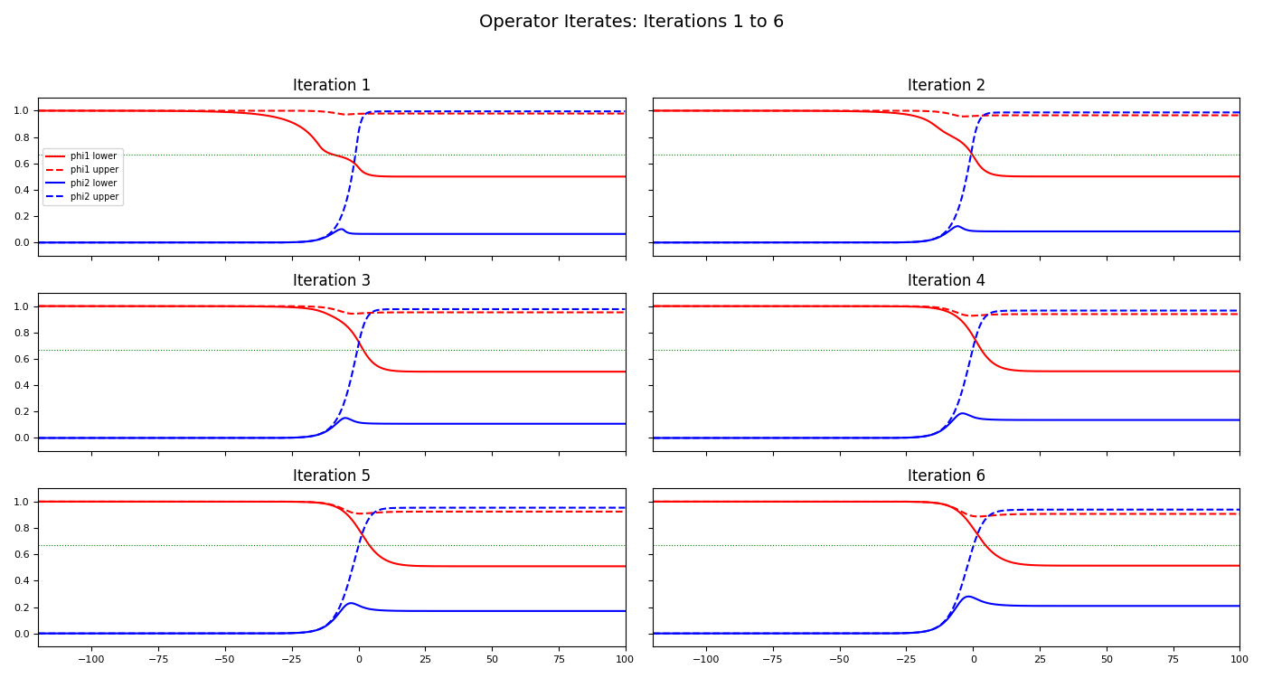
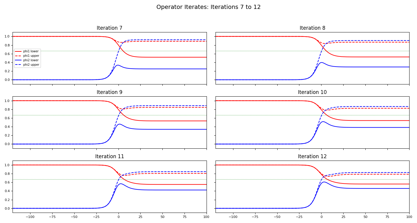
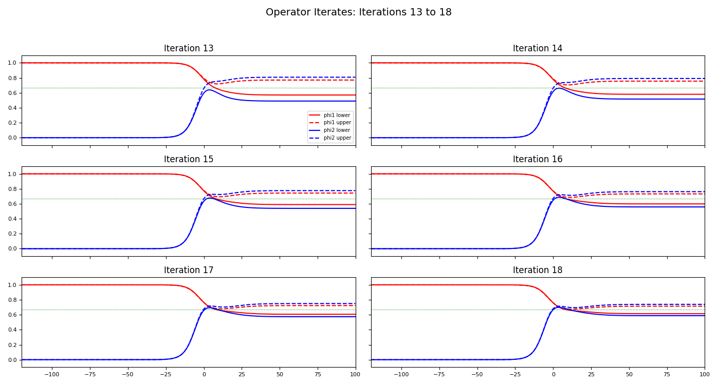
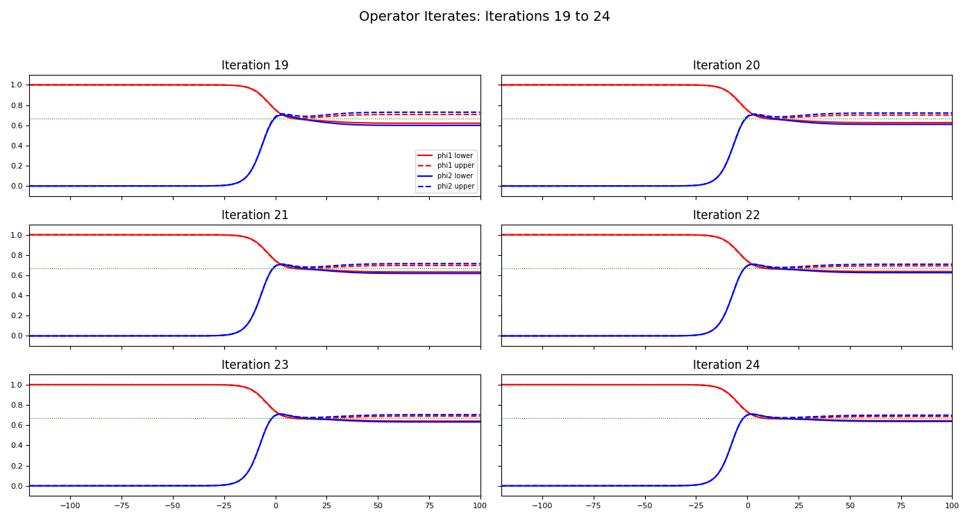
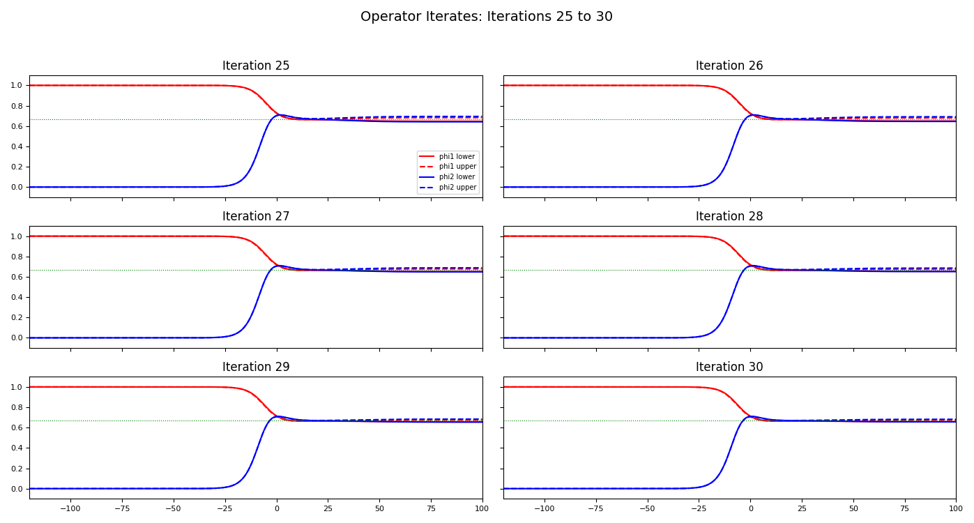
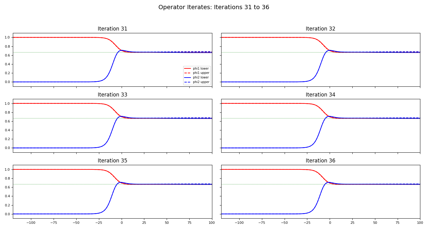
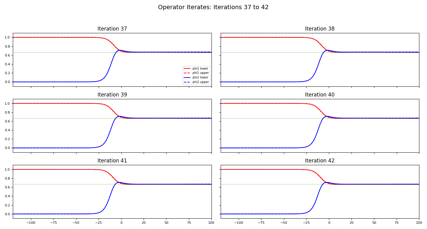
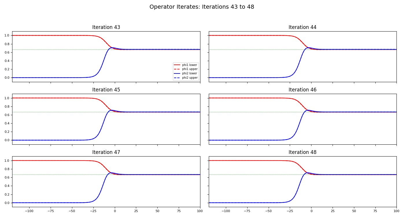
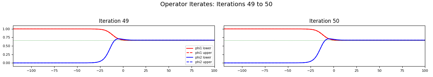
In this article, we establish the existence of traveling wave solutions for an invasive competition model with nonlocal diffusion and a Leslie-Gower response, incorporating time delays. We rigorously demonstrate the connection between super/sub-solutions and upper/lower solutions. Explicit constructions of super- and sub-solutions are provided, along with numerical simulations illustrating the behavior of the system.