
Competition is a very common ecological interaction in the natural world. It often occurs when species living in the same ecosystem have similar habits and lifestyles. A typical example of such a relationship is when paramecia in mixed cultivation compete for limited resources, such as food or living space. To accurately describe the dynamical behaviors of such a system, Lotka and Volterra independently proposed a now widely used model of interspecies competition for the first time respectively (see Ref. [1, 2]), that is, \[\label{eq1.1} \begin{cases} x'_1(t)=x_1(t)\Big[r_1-a_1x_1(t)-b_2x_2(t)\Big],\\ x'_2(t)=x_2(t)\Big[r_2-a_2x_2(t)-b_1x_1(t)\Big], \end{cases} \tag{1}\] where \(x_i(t)\) represents the population density of the \(i\)th species at time \(t\), the positive coefficients \(r_1, r_2\) and \(a_1, a_2\) are the intrinsic growth rate and self-inhibition rate respectively, positive coefficients \(b_j\) measure the interspecific competitive effects of species \(x_j\) on species \(x_i\), \(i, j = 1,2\) and \(i \neq j\). In the classical competition model, \(x_i\) response to \(x_j\) is assumed to be increasingly monotonic, an inherent assumption meaning is that the more \(x_j\) there exist in the environment, the worse off the \(x_i\). When the two species compete for the same limited resources in a closed system, by the famous competitive exclusion principle, one is often at a definite advantage, the other is eliminated fairly rapidly. However, Ayala et al. indicated that the experimental determinations of drosophila population dynamics cannot be well explained by the classical Lotka-Volterra competition model and proposed several theoretical models of interspecies competition (see Ref. [3]). In the real life, this interaction between different species may be upper-bound. Based on this fact, many scholars have developed the following competitive model with saturation effect (see Ref. [3, 4]), that is, \[\begin{cases} x'_1(t)=x_1(t)\Big[r_1-a_1x_1(t)-\displaystyle\frac{b_2x_2(t)}{1+x_2(t)}\Big],\\ x'_2(t)=x_2(t)\Big[r_2-a_2x_2(t)-\displaystyle\frac{b_1x_1(t)}{1+x_1(t)}\Big]. \end{cases}\]
In despite of the limitation of the linear model, the classical competition model is widely used and it does give a fair representation of competition between protozoan species (see Ref. [5]).
On the other hand, more and more people have realized that the ecosystem in the natural world is inevitably perturbed by various environment noises, such as Gaussian white noise, L\(\acute{e}\)vy noise and regime-switching (see Ref. [6– 11]). So it is of great significance to reveal the influences of environment noises on the population dynamics. Especially, the environment fluctuations could be well approximated by Gaussian white noise (see Ref. [12, 13]). Recently, along this line of thought, the dynamical behaviors of competitive system and their extended versions have been widely reported by many authors (see Ref. [14– 27]). We usually postulated that the white noises mainly affect the growth rates of the populations and analyzed a stochastic competition model with initial value \(x_1(0)>0, x_2(0)>0\), that is, \[\label{eq1.2} \begin{cases} dx_1(t)=x_1(t)\Big[r_1-a_1x_1(t)-\displaystyle\frac{b_2x_2(t)}{1+x_2(t)}\Big]dt+\sigma_1x_1(t)dB_1(t),\\ dx_2(t)=x_2(t)\Big[r_2-a_2x_2(t)-\displaystyle\frac{b_1x_1(t)}{1+x_1(t)}\Big]dt+\sigma_2x_2(t)dB_2(t), \end{cases} \tag{2}\] where \(\sigma^2_i\) represent the intensities of white noise, \(B_i(t)\) are the standard Brownian motions defined on a complete probability space \((\Omega, \mathcal{F}, P)\) with a filtration \(\{\mathcal{F}_t\}_{t\geq 0}\) satisfying the usual conditions, i.e., it is increasing and right continuous while \(\mathcal{F}_0\) contains all P-null sets, and the term \(b_ix_i/(1+x_i)\) is the functional response function of the \(x_j\) to the density of \(x_i\), and moreover it is an increasing function with respect to \(x_i\) and has a saturation value for large enough \(x_i\), \(i=1,2\) and \(i\neq j\). Our focus here is not only the stochastic permanence but also the persistence in the mean and weak persistence, with a particular interest in the stationary distribution of system (2) and revealing the influences of white noise on population system.
The organization of this paper is as follows. In §2, we introduce several definitions and lemmas which will be used. In §3, we first prove the existence and uniqueness of the globally positive solution of system (2) with the positive initial value. Then we derive the sufficient conditions for the stochastic permanence, strongly persistence in the mean, weak persistence and extinction respectively in §4. In §5, we further discuss the existence and uniqueness of the stationary distribution of system (2) and show that the fluctuation around the positive equilibrium point is bounded under a small noise. In §6, we provide several numerical simulations to justify the analytical results. In the last section, The results which we obtained are summarized, and the limitations of system (2) are also discussed.
In this section, we introduce some definitions and lemmas which will be used for establishing our main results.
Definition 1. The population \(x_i\) is said to be extinct with probability one if for any initial condition \(x_i(0)>0\), the solution \(x_i(t)\) has the property that \(\lim_{t\rightarrow\infty}x_i(t)=0, i=1,2\), almost surely.
Definition 2. The population \(x_i\) is said to be weakly persistent if \(\limsup_{t\rightarrow\infty}x_i(t) > 0, i=1,2\), almost surely.
Definition 3. (see Ref. [28]). System (2) is said to be stochastically permanent if for any \(\varepsilon\in(0,1)\), there exists a pair of positive constants \(\alpha,\beta\) such that for any initial condition \(x_i(0)>0\), the solution \(x_i(t), i=1,2\), has the property that \[\liminf_{t\rightarrow\infty}P\{x_i(t)\geq\alpha\}\geq1-\varepsilon,\ \liminf_{t\rightarrow\infty}P\{x_i(t)\leq\beta\}\geq1-\varepsilon.\]
Lemma 1. (see Ref. [29]). Suppose \(z(t)\in C[\Omega\times R_+, R_+]\), where \(R_+:= \{a|a >0, a\in R\}\).
(1) If there exist positive constants \(\lambda_0, T\) such that \[\ln z(t)\leq\lambda t-\lambda_0\int_0^tz(s)ds+\sum\limits_{i=1}^n\rho_iB_i(t),\] for \(t\geq T\), where \(\rho_i\) is a constant, then \[\limsup_{t\rightarrow\infty}\frac{\int_0^tz(s)ds}{t}\leq\frac{\lambda}{\lambda_0}\ a.s.,\] for \(\lambda \geq 0\).
(2) If there exist positive constants \(\lambda_0, T\) and \(\lambda\) such that \[\ln z(t)\geq\lambda t-\lambda_0\int_0^tz(s)ds+\sum\limits_{i=1}^n\rho_iB_i(t),\] for \(t\geq T\), where \(\rho_i\) is a constant, then \[\liminf_{t\rightarrow\infty}\frac{\int_0^tz(s)ds}{t}\geq\frac{\lambda}{\lambda_0}\ a.s..\]
Since \(x_i(t)\) denotes the population density of the \(i\)th species at time \(t\), and we mainly analysis the long-term behavior of system (2), so it is essential to require that the solution of system (2) is not only positive but also not explode in a finite time for the biological significance. For this reason, we will prove the existence and uniqueness of the globally positive solution in this section.
Theorem 1. For any given initial condition \(x_i(0)>0\), system (2) has a unique solution \(x_i(t)>0, i=1,2\), for all \(t\geq0\).
Proof. To begin with, let us consider the following stochastic system \[\label{eq3.1} \begin{cases} d\phi_1(t)=\Big[r_1-0.5\sigma^2_1-a_1e^{\phi_1(t)}-\displaystyle\frac{b_2e^{\phi_2(t)}}{1+e^{\phi_2(t)}}\Big]dt+\sigma_1dB_1(t),\\ d\phi_2(t)=\Big[r_2-0.5\sigma^2_2-a_2e^{\phi_2(t)}-\displaystyle\frac{b_1e^{\phi_1(t)}}{1+e^{\phi_1(t)}}\Big]dt+\sigma_2dB_2(t), \end{cases} \tag{3}\] with initial condition \(\phi_1(0)=\ln x_1(0), \phi_2(0)=\ln x_2(0)\). It is easy to see that the coefficients of system (3) satisfy the local Lipschitz condition, then system (3) has a unique solution \(\phi(t)\) on \([0, \tau_e)\), where \(\tau_{e}\) is the explosion time (see [30]). According to It\(\hat{o}\)’s formula, it is obvious that \(x_1(t)=e^{\phi_1(t)}, x_2(t)=e^{\phi_2(t)}\) is the unique positive local solution to system (2) with initial value \(x(0)\in R^2_+\). To show this solution is global, we only need to show that \(\tau_{e}=\infty\).
Let \(k_0>0\) be sufficiently large such that \(|x(0)|<k_0\). For each integer \(k\geq k_0\), we define the stopping time \[\tau_{k}=\inf\big\{t\in[0,\tau_e): |x(t)|>k\big\}.\]
Obviously, \(\tau_{k}\) is increasing as \(k\rightarrow\infty\). Let \(\tau_{\infty}=\lim_{k\rightarrow+\infty}\tau_{k}\), whence \(\tau_{\infty}\leq \tau_{e}\), if we can show that \(\tau_{\infty}=\infty\ a.s.\), then \(\tau_{e}=\infty\ a.s.\), the proof is completed.
Define a \(C^{2}\)-function \(\widetilde{V}(x): R^2_{+}\rightarrow R_{+}\) as \[\widetilde{V}(x_1, x_2)=x_1-1-\ln x_1+x_2-1-\ln x_2.\]
The nonnegative of this function can be seen from \(\varrho-1-\ln \varrho\geq0\) for \(\varrho>0\). Let \(T>0\) be an arbitrary constant, for \(0\leq t\leq\tau_{k}\wedge T\), applying It\(\hat{o}\)’s formula we obtain that
\[\begin{aligned} d\widetilde{V} &=(1-\frac{1}{x_1})dx_1+0.5\frac{1}{x_1^{2}}(dx_1)^{2}+(1-\frac{1}{x_2})dx_2+0.5\frac{1}{x_2^{2}}(dx_2)^{2}\notag\\ &=(x_1-1)(r_1-a_1x_1-\frac{b_2x_2}{1+x_2})dt+(x_1-1)\sigma_1dB_1(t)+\frac{1}{2}\sigma^2_1dt\notag\\ &\quad+(x_2-1)(r_2-a_2x_2-\frac{b_1x_1}{1+x_1})dt+(x_2-1)\sigma_2dB_2(t)+\frac{1}{2}\sigma^2_2dt, \end{aligned} \tag{4}\] that is, \[d\widetilde{V}\leq G(x_1,x_2)dt+(x_1-1)\sigma_1dB_1(t)+(x_2-1)\sigma_2dB_2(t),\] where \[G(x_1,x_2)=-a_1x_1^2+(r_1+a_1)x_1+b_1+\frac{1}{2}\sigma^2_1-r_1-a_2x_2^2+(r_2+a_2)x_2+b_2+\frac{1}{2}\sigma^2_2-r_2.\]
Clearly, \(G(x_1,x_2)\leq M\), where \(M\) is a positive constant. So we have \[d\widetilde{V}(x_1,x_2)\leq Mdt+(x_1-1)\sigma_1dB_1(t)+(x_2-1)\sigma_2dB_2(t).\]
Integrating from \(0\) to \(\tau_k \wedge T\) and then taking expectations on both sides yields that \[\begin{aligned} \label{eq3.3} E[\widetilde{V}(x_1(\tau_k \wedge T),x_2(\tau_k \wedge T))] &\leq\widetilde{V}(x_1(0),x_2(0))+ME(\tau_k \wedge T)\notag\\ &\leq\widetilde{V}(x_1(0),x_2(0))+MT. \end{aligned} \tag{5}\]
For any given \(l>0\), we define \[\mu(l)=\inf\{\widetilde{V}(x): |x|\geq l\}.\]
Then it is easy to see that \[\label{eq3.4} \lim_{l\rightarrow\infty}\mu(l)=\infty. \tag{6}\]
From (5) and the definition of \(\mu(l)\), we obtain that \[\label{eq3.5} \begin{aligned} \mu(k)P(\tau_k\leq T) \leq E[\widetilde{V}(x_1(\tau_{k}), x_2(\tau_{k}))1_{\Omega_{k}}]\leq \widetilde{V}(x_1(0),x_2(0))+MT, \end{aligned} \tag{7}\] where \(1_{\Omega_{k}}\) is the indicator function of \(\Omega_{k}:=\{\tau_{k}\leq T\}\). Letting \(k\rightarrow\infty\) and using (6) and (7) leads to \[P(\tau_{\infty}\leq T)=0.\]
By the arbitrariness of \(T\), we must have \[P(\tau_{\infty}=\infty)=1.\]
This completes the proof of Theorem 1. ◻
The long-term survival of each component is a basic question in population biology due to its theoretical and practical importance. As a result, we devote to establishing the sufficient conditions for stochastic permanence, weak persistence and extinction of system (2) in this section.
Theorem 2. Assume that \(x(t)\) is a solution of system (2), then for any \(q>1\), there exists a positive constant \(K=K(q)\) such that \[\limsup_{t\rightarrow\infty}E|x(t)|^q\leq K,\ i=1, 2.\]
Proof. Define \[V(x_1, x_2)=x^q_1+x^q_2,\] then by It\(\hat{o}\)’s formula we have \[\begin{aligned} \label{eq4.1} dV&=qx^{q-1}_1dx_1+0.5q(q-1)x_1^{q-2}(dx_1)^2+qx^{q-1}_2dx_2+0.5q(q-1)x_2^{q-2}(dx_2)^2\notag\\ &=\sum^2_{i=1}qx^{q}_i\Big[r_i-a_ix_i-\frac{b_jx_j}{1+x_j}+0.5(q-1)\sigma^2_i\Big]dt+q\sigma_1x^q_1dB_1(t)+q\sigma_2x^q_2dB_2(t)\notag\\ &\quad\leq \big[\mathcal{L}(x_1, x_2)-V\big]dt+q\sigma_1x^q_1dB_1(t)+q\sigma_2x^q_2dB_2(t), \end{aligned} \tag{8}\] where \[\mathcal{L}(x_1, x_2)=\sum^2_{i=1}x^{q}_i\big[1+qr_i+0.5q(q-1)\sigma^2_i-a_iqx_i\big].\]
It is obvious that there is a positive constant \(K_1=K_1(q)\) such that \(\mathcal{L}(x_1,x_2)\leq K_1,\) where \[K_1=\sum^2_{i=1}\frac{\big[1+qr_i+0.5q(q-1)\sigma^2_i\big]^{q+1}}{(q+1)^{q+1}a_i^q}.\]
Making use of It\(\hat{o}\)’s formula to \(e^tV(x_1,x_2)\) yields that \[\label{eq4.2} \begin{aligned} d[e^tV(x_1,x_2)]&=e^tV(x_1,x_2)dt+e^tdV(x_1,x_2)\leq K_1e^tdt+e^tq\sigma_1x^q_1dB_1(t)+e^tq\sigma_2x^q_2dB_2(t). \end{aligned} \tag{9}\]
Then integrating from \(0\) to \(t\) and taking expectations on both sides leads to \[e^tE[V(x_1,x_2)]\leq V(x_1(0),x_2(0))+K_1(e^t-1).\]
This implies \[\limsup_{t\rightarrow\infty}E[V(x_1,x_2)]\leq K_1.\]
On the other hand, because \(|x(t)|^q\leq2^{q-1}V(x_1,x_2)\), so we have \[\limsup_{t\rightarrow\infty}E|x(t)|^q\leq2^{q-1}\limsup_{t\rightarrow\infty}E[V(x_1,x_2)]\leq 2^{q-1}K_1=K.\]
This completes the proof of Theorem 2. ◻
It follows directly from Theorem 2 together with Chebyshev’s inequality that system (2) is stochastically ultimate boundedness. We describe it as a theorem below.
Theorem 3. Assume that \(x(t)\) is a solution of system (2) with initial condition \(x(0)\in R^2_{+}\), then for any \(\varepsilon\in(0,1)\), there exists a positive constant \(\beta=\beta(\varepsilon)\) such that \[\limsup_{t\rightarrow\infty}P\{|x(t)|>\beta\}\leq\varepsilon. \tag{10}\]
Proof. Let \(\beta=(\frac{K}{\varepsilon})^{\frac{1}{q}}\), then by Chebyshev’s inequality, we have \[P\{|x(t)|>\beta\}\leq\frac{E[|x(t)|^q]}{\beta^q}.\]
Therefore, we have \[\limsup_{t\rightarrow\infty}P\{|x(t)|>\beta\}\leq\varepsilon.\]
This completes the proof of Theorem 3. ◻
Next we turn to discuss the critical value for stochastic permanence of system (2).
Theorem 4. If \(r_1>b_2+0.5\sigma_1^2\) and \(r_2>b_1+0.5\sigma_2^2\) hold, then system (2) is stochastically permanent for any initial condition \(x_1(0)>0\) and \(x_2(0)>0\).
Proof. Assign \(0<\varepsilon<1\) arbitrarily, we first show that there is a positive constant \(\beta=\beta(\varepsilon)\) such that \[\liminf_{t\rightarrow\infty}P\{x_i(t)\leq\beta\}\geq1-\varepsilon.\]
From Theorem 3, we can see that \[\limsup_{t\rightarrow\infty}E[x^q_i(t)]\leq\limsup_{t\rightarrow\infty}E|x(t)|^q\leq K.\]
Then it is easy to obtain the desired assertion by Chebyshev’s inequality.
In the following, we only need to prove that for arbitrary \(\varepsilon\in(0,1)\), there is a positive constant \(\alpha=\alpha(\varepsilon)\) such that \[\liminf_{t\rightarrow\infty}P\{x_i(t)\geq\alpha\}\geq1-\varepsilon.\]
It follows from \(r_i>b_j+0.5\sigma_i^2\) that we can choose a constant \(\theta > 0\) such that \[r_i-b_j-0.5\sigma_i^2-0.5\theta\sigma_i^2>0,\ i\neq j,\ i,j=1,2.\]
Define \[V_1(x_1,x_2)=\sum^2_{i=1}\frac{1}{\theta}\big(1+\frac{1}{x_i}\big)^\theta.\]
By It\(\hat{\text{o}}\)’s formula, One derives that \[\begin{aligned} \label{eq4.4} dV_1 &=\sum^2_{i=1} (1+x_i^{-1})^{\theta-1}dx_i^{-1}+\sum^2_{i=1}0.5(\theta-1)(1+x_i^{-1})^{\theta-2}(dx_i^{-1})^2\notag\\ &=\sum^2_{i=1} (1+x_i^{-1})^{\theta-2}\Big\{-(1+x_i^{-1})x_i\Big[r_i-a_ix_i-\frac{b_jx_j}{1+x_j}-\sigma^2_i\Big]\notag\\ &\quad+0.5(\theta-1)\sigma^2_ix_i^{-2}\Big\}dt-\sum^2_{i=1}\sigma_ix_i^{-1}(1+x_i^{-1})^{\theta-1}dB_i(t)\notag\\ &\leq\sum^2_{i=1}(1+x_i^{-1})^{\theta-2}\Big\{-x_i^{-2}(r_i-b_j-0.5\sigma_i^2-0.5\theta\sigma_i^2)\notag\\ &\quad+x_i^{-1}(b_j+a_i+\sigma_i^2-r_i)+a_i\Big\}dt-\sum^2_{i=1}\sigma_ix_i^{-1}(1+x_i^{-1})^{\theta-1}dB_i(t). \end{aligned} \tag{11}\]
Let \(\kappa\) be sufficiently small to satisfy \[0<\dfrac{\kappa}{\theta}<r_i-b_j-0.5\sigma_i^2-0.5\theta\sigma_i^2,\ i\neq j,\ i,j=1,2.\]
We continue to define \[V_2(t, x_1, x_2)=e^{\kappa t}V_1(x_1, x_2).\]
By virtue of It\(\hat{o}\)’s formula, we obtain that \[\begin{aligned} \label{eq4.5} dV_2&=\kappa e^{\kappa t}V_1dt+e^{\kappa t}dV_1\nonumber\\ &\leq\sum^2_{i=1}e^{\kappa t}(1+x_i^{-1})^{\theta-2}\Big\{\frac{\kappa}{\theta}(1+x_i^{-1})^{2}-x_i^{-2}(r_i-b_j-0.5\sigma_i^2-0.5\theta\sigma_i^2)\nonumber\\ &\quad+x_i^{-1}(b_j+a_i+\sigma_i^2-r_i)+a_i\Big\}dt-\sum^2_{i=1}\sigma_ix_i^{-1}(1+x_i^{-1})^{\theta-1}e^{\kappa t}dB_i(t)\nonumber\\ &=e^{\kappa t}G(x_1, x_2)dt-\sum^2_{i=1}\sigma_ix_i^{-1}(1+x_i^{-1})^{\theta-1}e^{\kappa t}dB_i(t), \end{aligned} \tag{12}\] where \[\begin{aligned} G(x_1,x_2)=\sum^2_{i=1}(1+x_i^{-1})^{\theta-2}\Big\{-x_i^{-2}\left(r_i-b_j-0.5\sigma_i^2-0.5\theta\sigma_i^2-\frac{\kappa}{\theta}\right)+x_i^{-1}\left(b_j+a_i+\sigma_i^2-r_i+\frac{2\kappa}{\theta}\right)+a_i+\frac{\kappa}{\theta}\Big\}. \end{aligned}\]
Now we turn to verifying \(G(x_1,x_2)\) is upper bounded. Assign \[A_i=r_i-b_j-0.5\sigma_i^2-0.5\theta\sigma_i^2-\frac{\kappa}{\theta}, B_i=b_j+a_i+\sigma_i^2-r_i+\frac{2\kappa}{\theta}, C_i=a_i+\frac{\kappa}{\theta},\] then \(G(x_i)=(1+x_i^{-1})^{\theta-2}(-A_ix_i^{-2}+B_ix_i^{-1}+C_i)=(1+x_i^{-1})^{\theta-2}\tilde{G}(x_i)\).
Let \[\mathcal{X}=\frac{B_i+\sqrt{B_i^2+4A_iC_i}}{2A_i},\ \mathcal{U}=\frac{B_i^2+4A_iC_i}{4A_i}.\]
If \(\dfrac{1}{x_i}\geq\mathcal{X}\), then \(\tilde{G}(x_i)\leq0\) and so \(G(x_i)\leq0\). If \(0<\displaystyle\frac{1}{x_i}\leq\mathcal{X}\), then \(\tilde{G}(x_i)\leq\mathcal{U}\). For \(\theta\geq2\), \((1+x_i^{-1})^{\theta-2}\leq(1+\mathcal{X})^{\theta-2}\), while \((1+x_i^{-1})^{\theta-2}\leq1\) for \(0<\theta<2\). So \(G(x_1,x_2)\) is upper bounded, we denote it \(\mathcal{R}\).
Now we return to (12) yields that \[\label{eq4.6} \begin{aligned} dV_2&\leq e^{\kappa t}\mathcal{R}dt-\sum^2_{i=1}\sigma_ix_i^{-1}(1+x_i^{-1})^{\theta-1}e^{\kappa t}dB_i(t). \end{aligned} \tag{13}\]
Integrating from \(0\) to \(t\) and taking expectations on both sides, then we obtain that \[\label{eq4.7} EV_2=e^{\kappa t}E[V_1(x_1,x_2)]\leq V_1(x_1(0),x_2(0))+\frac{\mathcal{R}}{\kappa}(e^{\kappa t}-1). \tag{14}\]
This implies that \[\label{eq4.8} \begin{aligned} \limsup_{t\rightarrow\infty}E[V_1(x_1,x_2)]\leq\frac{\mathcal{R}}{\kappa}. \end{aligned} \tag{15}\]
Furthermore, \[\label{eq4.9} \begin{aligned} \limsup_{t\rightarrow\infty}E[x^{-\theta}_i(t)] \leq\limsup_{t\rightarrow\infty}E\left[\left(1+\frac{1}{x_i}\right)^{\theta}\right]\leq\theta\limsup_{t\rightarrow\infty}E[V_1(x_1,x_2)] \leq\frac{\theta\mathcal{R}}{\kappa}:=\delta. \end{aligned} \tag{16}\]
For arbitrary \(\varepsilon\in (0, 1)\), let \(\alpha=\displaystyle(\frac{\varepsilon}{\delta})^{\frac{1}{\theta}}\), by Chebyshevs inequality, we have \[P\{x_i(t)<\alpha\}=P\{x^{-\theta}_i(t)>\alpha^{-\theta}\}\leq\frac{E[x^{-\theta}_i(t)]}{\alpha^{-\theta}}=\alpha^{\theta}E[x^{-\theta}_i(t)].\] This gives that \[\limsup_{t\rightarrow\infty}P\{x_i(t)<\alpha\}\leq\alpha^{\theta}\delta=\varepsilon.\]
That is \[\liminf_{t\rightarrow\infty}P\{x_i(t)\geq\alpha\}\geq1-\varepsilon.\] This completes the proof of Theorem 4. ◻
To end this section, we discuss the extinction and weak persistence of system (2) and estimate the limit of the average in time of the sample paths of every component.
Theorem 5. Assume that \(x(t)=(x_1(t), x_2(t))\) is a solution of system (2) with initial value \((x_1(0), x_2(0))\in R_+^2\), then the component \(x_i(t)\) has the following properties.
(1) If \(r_i>0.5\sigma^2_i+b_j\), then \[\liminf_{t\rightarrow\infty}\frac{\int_0^tx_i(s)ds}{t}\geq\frac{r_i-0.5\sigma^2_i-b_j}{a_i}\ a.s..\] In other words, population \(x_i\) is strongly persistence in the mean almost surely.
Moreover, \[\limsup_{t\rightarrow\infty}\frac{\int_0^tx_i(s)ds}{t}\leq\frac{r_i-0.5\sigma^2_i}{a_i}\ a.s..\]
(2) If \(r_i<0.5\sigma^2_i\), then population \(x_i\) goes to extinction almost surely.
(3) If \(r_i>0.5\sigma^2_i\), then population \(x_i\) is weakly persistent almost surely.
Proof. (1) An application of It\(\hat{o}\)’s formula to system (2) yields that \[\label{eq4.10} \begin{aligned} d\ln x_i(t)=\frac{1}{x_i}dx_i-\frac{(dx_i)^2}{2x^2_i}=\left[r_i-0.5\sigma^2_i-a_ix_i-\frac{b_jx_j}{1+x_j}\right]dt+\sigma_idB_i(t), \end{aligned} \tag{17}\] that is, \[\label{eq4.11} \ln x_i(t)-\ln x_i(0)= (r_i-0.5\sigma^2_i)t-a_i\int_0^tx_i(s)ds-b_j\int_0^t\frac{x_j(s)}{1+x_j(s)}ds+\sigma_iB_i(t). \tag{18}\]
It follows from (18) that \[\label{eq4.12} \ln x_i(t)-\ln x_i(0)\geq (r_i-0.5\sigma^2_i-b_j)t-a_i\int_0^tx_i(s)ds+\sigma_iB_i(t). \tag{19}\]
Noticed that \(\lim\limits_{t\rightarrow\infty}\frac{\ln x_i(0)}{t}=0\), then by (2) in Lemma 1, we obtain that \[\liminf_{t\rightarrow\infty}\frac{\int_0^tx_i(s)ds}{t}\geq\frac{r_i-0.5\sigma^2_i-b_j}{a_i}\ a.s..\]
On the other hand, \[\label{eq4.13} \ln x_i(t)-\ln x_i(0)\leq(r_i-0.5\sigma^2_i)t-a_i\int_0^tx_i(s)ds+\sigma_iB_i(t), \tag{20}\] then by (1) in Lemma 1, we obtain that \[\limsup_{t\rightarrow\infty}\frac{\int_0^tx_i(s)ds}{t}\leq\frac{r_i-0.5\sigma^2_i}{a_i}\ a.s..\]
(2) Let \(\gamma_i(t)\) be the solution of equation \[\label{eq4.14} d\gamma_i(t)=\gamma_i(t)[r_i-a_i\gamma_i(t)]dt+\sigma_i\gamma_i(t)dB_i(t), i=1,2, \tag{21}\] with \(\gamma_i(0)=x_i(0)\), then equation (21) has explicit solution of the form \[\label{eq4.15} \gamma_i(t)=\frac{\exp[(r_i-\sigma^2_i/2)t+\sigma_iB_i(t)]}{1/\gamma_i(0)+a_i\int_0^t\exp[(r_i-\sigma^2_i/2)s+\sigma_iB_i(s)]ds}. \tag{22}\]
According to the comparison theorem of stochastic equations (see Ref. [31]), we know that \(x_i(t)\leq \gamma_i(t)\). If \(r_i<0.5\sigma^2_i\), it then follows from (22) that \[\label{eq4.16} x_i(t)\leq \gamma_i(t)\leq \gamma_i(0)\exp\big\{t[r_i-\sigma^2_i/2+\sigma_iB_i(t)/t]\big\}, \tag{23}\] in view of \(\lim_{t\rightarrow\infty}\frac{B_i(t)}{t}=0\), then we have \(\displaystyle\lim_{t\rightarrow\infty}\gamma_i(t)\leq0\). In other words, \(\displaystyle\lim_{t\rightarrow\infty}x_i(t)=0\).
(3) By the comparison theorem of stochastic equations, we obtain that \[\label{eq4.17} 0 < x_i(t)\leq \gamma_i(t). \tag{24}\]
Hence, to complete the proof, we need to show that \(\limsup\limits_{t\rightarrow\infty}\gamma_i(t)>0\). In fact, if \(\limsup\limits_{t\rightarrow\infty}\gamma_i(t)=0\), then from the squeeze rule of the limit we must have \(\limsup\limits_{t\rightarrow\infty}x_i(t)=0\).
From equation (21), we have \[\label{eq4.18} d\ln\gamma_i(t)=[r_i-0.5\sigma^2_i-a_i\gamma_i(t)]dt+\sigma_idB_i(t), \tag{25}\] which gives that \[\label{eq4.19} \frac{\ln \gamma_i(t)-\ln \gamma_i(0)}{t}=(r_i-0.5\sigma^2_i)-a_i\frac{1}{t}\int_0^t\gamma_i(s)ds+\sigma_i\frac{B_i(t)}{t}. \tag{26}\]
Denote the set \(S\) by \(\{\omega: \limsup\limits_{t\rightarrow\infty}\gamma_i(t)=0\}\), and we assume that \(P(S)>0\). Then for \(\forall\ \omega\in S\), we have \(\limsup_{t\rightarrow\infty}\gamma_i(t, \omega)=0\). And then for arbitrary \(\varepsilon\) satisfying \(0<\varepsilon<1\), there exists a \(T(\omega)\) such that \[\label{eq4.20} \gamma_i(t, \omega)\leq\varepsilon\ \text{for}\ t\geq T(\omega). \tag{27}\]
It then follows that \[\label{eq4.21} \limsup_{t\rightarrow\infty}\frac{\ln \gamma_i(t)-\ln \gamma_i(0)}{t}\leq0. \tag{28}\]
Recalling (27), we obtain from the continuity of \(\gamma_i(t,\omega)\) that there exists a constant \(\tilde{K}\) such that \(\gamma_i(t,\omega)\leq\tilde{K}\) for \(0\leq t\leq T(\omega)\). On the other hand, \[\label{eq4.22} \begin{aligned} \frac{1}{t}\int_0^t\gamma_i(s,\omega)ds &= \frac{1}{t}\int_0^{T(\omega)}\gamma_i(s,\omega)ds+\frac{1}{t}\int_{T(\omega)}^{t}\gamma_i(s,\omega)ds\leq \tilde{K}\frac{T(\omega)}{t}+\varepsilon\frac{t-T(\omega)}{t}, \end{aligned} \tag{29}\] for sufficient large \(t\). Since \(\varepsilon\) is arbitrarily small, we obtain that \[\label{eq4.23} \limsup_{t\rightarrow\infty}\frac{1}{t}\int_0^t\gamma_i(s,\omega)ds\leq 0. \tag{30}\]
In view of that \(\gamma_i(t)>0\), \(\liminf_{t\rightarrow\infty}\frac{1}{t}\int_0^t\gamma_i(s,\omega)ds\geq 0\), so we have \[\label{eq4.24} \lim_{t\rightarrow\infty}\frac{1}{t}\int_0^t\gamma_i(s,\omega)ds=0. \tag{31}\]
Substituting (31) into (26) and making use of the strong law of large numbers, one can deduce the contradiction that \[\label{eq4.25} \limsup_{t\rightarrow\infty}\frac{\ln \gamma_i(t)-\ln \gamma_i(0)}{t}=r_i-0.5\sigma^2_i>0. \tag{32}\]
Recalling the above discussion, we can obtain that \(\limsup_{t\rightarrow\infty}x_i(t)>0\). This completes the proof of Theorem 5. ◻
Remark 1. Theorem 4 and 5 reveal that \(r_i=0.5\sigma^2_i\) is the threshold of extinction and weak persistence. And the permanence of system (2) depends on the intensities of the random perturbations, that is, a small stochastic perturbation does not alter the permanence of the species, but a large one will force the species incline to extinction with probability one.
In the following, we prove the existence of stationary distribution for system (2) by using the Hasminskiis methods. To begin with, let us make some preparations.
Let \(x(t)\) be a homogeneous Markov process defined in \(E_l\) (\(l\) dimensional Euclidean space) described by the following stochastic equation \[dx(t)=b(x)dt+\sum\limits_{r=1}^k\sigma_r(x)dB_r(t).\]
The diffusion matrix is \[A(x)=(a_{ij}(x)),a_{ij}(x)=\sum\limits_{r=1}^k\sigma^i_r(x)\sigma^j_r(x).\]
Definition 4. Let \(P(t,x,\cdot)\) be the probability measure induced by \(x(t)\) with initial value \(x(0)\), that is, \[P(t,x,\Delta)=P\big(x(t)\in \Delta|x(0)\big),\] for any Borel set \(\Delta\subset R^2_+\). If there exists a probability measure \(\nu(\cdot)\) such that \[\lim\limits_{t\rightarrow\infty}P(t,x,\Delta)=\nu(\Delta),\] for all \(x\in R^2_+\), then we say that the Markov process \(x(t)\) has a stationary distribution \(\nu(\cdot)\).
Assumption 1. There exists a bounded domain \(U\subset E_l\) with regular boundary \(\Gamma\), having the following properties:
(1) In the domain \(U\) and some neighborhood thereof, the smallest eigenvalue of the diffusion matrix \(A(x)\) is bounded away from zero.
(2) If \(x\in E_l\backslash \bar{U}\), the mean time \(\tau\) at which a path issuing from \(x\) reaches the set \(U\) is finite, and \(\sup_{x\in K} E_x\tau<\infty\) every compact subset \(K\subset E_l\).
Lemma 2. (see Ref. [32]). If Assumption 1 holds, then the Markov process \(x(t)\) has a unique stationary distribution \(\nu(\cdot)\).
Remark 2. The proof of the above lemma can be found at page 134 of Ref. [32]. For the existence of a stationary distribution with suitable density function, we refer to Theorem 4.1 at page 119 and Lemma 9.4 at page 138 in Ref. [32].
To validate (1), it is sufficient to prove that \(F\) is uniformly elliptical in \(U\), where \[Fu=b(x)\cdot u_x+[tr(A(x)u_{xx})]/2,\] that is, there is a positive number \(M\) such that \(\sum\limits_{i,j=1}^la_{ij}(x)\lambda_i\lambda_j\geq M|\lambda|^2\) for any \(x\in U\) and \(\lambda\in R_l\) (see Chapter 3, page 103 of Ref. [33] and Rayleigh’s principle in Ref. [34], Chapter 6, page 349).
To verify (2), it is enough to show that there exists a neighborhood \(U\) and a non-negative \(C^2\)-function \(V\) such that for any \(x\in E_l\backslash \bar{U}\), \(LV(x)\) is negative, for more details, see page 1163 in Ref. [35].
Remark 3. System (2) can be written as the following form \[\begin{aligned}d\left( \begin{array}{c} x_1(t)\\ x_2(t)\\ \end{array} \right)= \left( \begin{array}{c} x_1(t)\left[r_1-a_1x_1(t)-\dfrac{b_2x_2(t)}{1+x_2(t)}\right]\\ x_2(t)\left[r_2-a_2x_2(t)-\dfrac{b_1x_1(t)}{1+x_1(t)}\right]\\ \end{array} \right)dt&+\left( \begin{array}{c} \sigma_1x_1(t)\\ 0\\ \end{array} \right)dB_1(t)+\left( \begin{array}{c} 0\\ \sigma_2x_2(t)\\ \end{array} \right)dB_2(t),\end{aligned}\] and the diffusion matrix is \[A=diag(\sigma^2_1x^2_1(t),\sigma^2_2x^2_2(t)).\]
Remark 4. Let \((\hat{x}_1, \hat{x}_2)\) be the positive equilibrium point of system (1), then it follows that \[\label{eq5.1} \begin{cases} r_1=a_1\hat{x}_1+\dfrac{b_2\hat{x}_2}{1+\hat{x}_2},\\ r_2=a_2\hat{x}_2+\dfrac{b_1\hat{x}_1}{1+\hat{x}_1}. \end{cases} \tag{33}\]
Theorem 6. Let \((x_1(t),x_2(t))\) be the solution of system (2) with initial value \((x_1(0),x_2(0))\in R^2_+\), if \[\eta_1>\frac{\beta}{2},\ \eta_2>\frac{\beta}{2},\] and \[\label{h2} 0<\sigma<\min\Big\{(\eta_1-\frac{\beta}{2})\hat{x}^2_1,\ (\eta_2-\frac{\beta}{2})\hat{x}^2_2\Big\}, \tag{34}\] where \[\begin{split} \eta_1 &= a_1(1+\hat{x}_2),\ \eta_2 = a_2(1+\hat{x}_1),\ \beta = b_1+b_2,\\ \sigma &= \frac{1}{2}\sigma^2_1\hat{x}_1(1+\hat{x}_2)+\frac{1}{2}\sigma^2_2\hat{x}_2(1+\hat{x}_1), \end{split}\] then system (2) has a unique stationary distribution \(\nu(\cdot)\).
Remark 5. Since \(\lim\limits_{\sigma_1,\sigma_2\rightarrow0}\sigma=0\), therefore, condition (34) is verified for sufficiently small environment noises.
Proof. From Theorem 1, we know that the solution \(x(t)\) is globally positive for any positive initial value. We then define a \(C^2\)-function \(V: R^2_+\rightarrow R_+\) as \[\begin{aligned} V(x_1,x_2) & =(1+\hat{x}_2)\Big(x_1-\hat{x}_1-\hat{x}_1\ln\frac{x_1}{\hat{x}_1}\Big)+(1+\hat{x}_1)\Big(x_2-\hat{x}_2-\hat{x}_2\ln\frac{x_2}{\hat{x}_2}\Big) =V_1+V_2, \end{aligned}\] where we write \(x(t)\) and \(y(t)\) as \(x\) and \(y\) respectively for simplicity. By It\(\hat{o}\)’s formula, we have \[\begin{aligned} \label{eq5.11} dV_1 = &(1+\hat{x}_2)(1-\frac{\hat{x}_1}{x_1})dx_1+\frac{1}{2}(1+\hat{x}_2)\dfrac{\hat{x}_1}{x^2_1}(dx_1)^2\notag\\ = &(1+\hat{x}_2)(x_1-\hat{x}_1)\Big[\Big(r_1-a_1x_1-\dfrac{b_2x_2}{1+x_2}\Big)dt+\sigma_1dB_1(t)\Big]+\frac{1}{2}\sigma^2_1\hat{x}_1(1+\hat{x}_2)dt\notag\\ = &(1+\hat{x}_2)(x_1-\hat{x}_1)\Big[\Big(a_1\hat{x}_1+\dfrac{b_2\hat{x}_2}{1+\hat{x}_2}-a_1x_1-\dfrac{b_2x_2}{1+x_2}\Big)dt\Big] +\frac{1}{2}\sigma^2_1\hat{x}_1(1+\hat{x}_2)dt+\sigma_1(1+\hat{x}_2)(x_1-\hat{x}_1)dB_1(t)\notag\\ = &(x_1-\hat{x}_1)\Big[(1+\hat{x}_2)a_1(\hat{x}_1-x_1)+\dfrac{b_2(\hat{x}_2-x_2)}{1+x_2}\Big]dt+\frac{1}{2}\sigma^2_1\hat{x}_1(1+\hat{x}_2)dt\notag+\sigma_1(1+\hat{x}_2)(x_1-\hat{x}_1)dB_1(t)\notag\\ = &\Big[-a_1(1+\hat{x}_2)(x_1-\hat{x}_1)^2+\dfrac{b_2(x_1-\hat{x}_1)(\hat{x}_2-x_2)}{1+x_2}+\frac{1}{2}\sigma^2_1\hat{x}_1(1+\hat{x}_2)\Big]dt+\sigma_1(1+\hat{x}_2)(x_1-\hat{x}_1)dB_1(t)\notag\\ = &LV_1dt+\sigma_1(1+\hat{x}_2)(x_1-\hat{x}_1)dB_1(t), \end{aligned} \tag{35}\] and \[\begin{aligned} \label{eq5.12} dV_2 = &(1+\hat{x}_1)(1-\frac{\hat{x}_2}{x_2})dx_2+\frac{1}{2}(1+\hat{x}_1)\dfrac{\hat{x}_2}{x^2_2}(dx_2)^2\notag\\ = &(1+\hat{x}_1)(x_2-\hat{x}_2)\Big[\Big(r_2-a_2x_2-\dfrac{b_1x_1}{1+x_1}\Big)dt+\sigma_2dB_2(t)\Big]+\frac{1}{2}\sigma^2_2\hat{x}_2(1+\hat{x}_1)dt\notag\\ = &(1+\hat{x}_1)(x_2-\hat{x}_2)\Big[\Big(a_2\hat{x}_2+\dfrac{b_1\hat{x}_1}{1+\hat{x}_1}-a_2x_2-\dfrac{b_1x_1}{1+x_1}\Big)dt\Big] +\frac{1}{2}\sigma^2_2\hat{x}_2(1+\hat{x}_1)dt+\sigma_2(1+\hat{x}_1)(x_2-\hat{x}_2)dB_2(t)\notag\\ = &(x_2-\hat{x}_2)\Big[a_2(1+\hat{x}_1)(\hat{x}_2-x_2)+\dfrac{b_1(\hat{x}_1-x_1)}{1+x_1}\Big]dt +\frac{1}{2}\sigma^2_2\hat{x}_2(1+\hat{x}_1)dt+\sigma_2(1+\hat{x}_1)(x_2-\hat{x}_2)dB_2(t)\notag\\ = &\Big[-a_2(1+\hat{x}_1)(x_2-\hat{x}_2)^2+\dfrac{b_1(x_2-\hat{x}_2)(\hat{x}_1-x_1)}{1+x_1}+\frac{1}{2}\sigma^2_2\hat{x}_2(1+\hat{x}_1)\Big]dt+\sigma_2(1+\hat{x}_1)(x_2-\hat{x}_2)dB_2(t)\notag\\ = &LV_2dt+\sigma_2(1+\hat{x}_1)(x_2-\hat{x}_2)dB_2(t). \end{aligned} \tag{36}\]
Then we have \[\label{eq5.13} \begin{aligned} dV & = dV_1+dV_2 = LVdt+\sigma_1(1+\hat{x}_2)(x_1-\hat{x}_1)dB_1(t)+\sigma_2(1+\hat{x}_1)(x_2-\hat{x}_2)dB_2(t), \end{aligned} \tag{37}\] where \[\begin{aligned} \label{eq5.14} LV = & -a_1(1+\hat{x}_2)(x_1-\hat{x}_1)^2+\dfrac{b_2(x_1-\hat{x}_1)(\hat{x}_2-x_2)}{1+x_2}+\frac{1}{2}\sigma^2_1\hat{x}_1(1+\hat{x}_2)\notag\\ & -a_2(1+\hat{x}_1)(x_2-\hat{x}_2)^2+\dfrac{b_1(x_2-\hat{x}_2)(\hat{x}_1-x_1)}{1+x_1}+\frac{1}{2}\sigma^2_2\hat{x}_2(1+\hat{x}_1)\notag\\ = & -\Big[a_1(1+\hat{x}_2)(x_1-\hat{x}_1)^2+\Big(\dfrac{b_2}{1+x_2}+\dfrac{b_1}{1+x_1}\Big)(x_1-\hat{x}_1)(x_2-\hat{x}_2)\notag\\ & +a_2(1+\hat{x}_1)(x_2-\hat{x}_2)^2\Big]+\frac{1}{2}\sigma^2_1\hat{x}_1(1+\hat{x}_2)+\frac{1}{2}\sigma^2_2\hat{x}_2(1+\hat{x}_1). \end{aligned} \tag{38}\]
Case 1. If \((x_1-\hat{x}_1)(x_2-\hat{x}_2)>0\), then we obtain that \[\label{eq5.6} \begin{split} LV \leq & -\Big[a_1(1+\hat{x}_2)(x_1-\hat{x}_1)^2+a_2(1+\hat{x}_1)(x_2-\hat{x}_2)^2\Big]+\frac{1}{2}\sigma^2_1\hat{x}_1(1+\hat{x}_2) +\frac{1}{2}\sigma^2_2\hat{x}_2(1+\hat{x}_1). \end{split} \tag{39}\]
Let \(\eta_1=a_1(1+\hat{x}_2), \eta_2=a_2(1+\hat{x}_1)\) and \(\sigma=\frac{1}{2}\sigma^2_1\hat{x}_1(1+\hat{x}_2)+\frac{1}{2}\sigma^2_2\hat{x}_2(1+\hat{x}_1)\), then \[\label{eq5.7} LV \leq -\eta_1(x_1-\hat{x}_1)^2-\eta_2(x_2-\hat{x}_2)^2+\sigma. \tag{40}\]
Case 2. If \((x_1-\hat{x}_1)(x_2-\hat{x}_2)<0\), it follows from (38) that \[\begin{aligned} \label{eq5.8} LV \leq & -\big[a_1(1+\hat{x}_2)(x_1-\hat{x}_1)^2+(b_2+b_1)(x_1-\hat{x}_1)(x_2-\hat{x}_2)\notag\\ & +a_2(1+\hat{x}_1)(x_2-\hat{x}_2)^2\big]+\frac{1}{2}\sigma^2_1\hat{x}_1(1+\hat{x}_2)+\frac{1}{2}\sigma^2_2\hat{x}_2(1+\hat{x}_1). \end{aligned} \tag{41}\]
Let \(\beta=b_2+b_1\), then we have \[\begin{aligned} \label{eq5.9} LV \leq &-\eta_1(x_1-\hat{x}_1)^2-\beta(x_1-\hat{x}_1)(x_2-\hat{x}_2)-\eta_2(x_2-\hat{x}_2)^2+\sigma\notag\\ \leq &-\eta_1(x_1-\hat{x}_1)^2+\beta|x_1-\hat{x}_1||x_2-\hat{x}_2|-\eta_2(x_2-\hat{x}_2)^2+\sigma\notag\\ \leq &-(\eta_1-\frac{\beta}{2})(x_1-\hat{x}_1)^2-(\eta_2-\frac{\beta}{2})(x_2-\hat{x}_2)^2+\sigma. \end{aligned} \tag{42}\]
Combining Case 1 and Case 2, we can then infer that \[\label{eq5.10} LV \leq -(\eta_1-\frac{\beta}{2})(x_1-\hat{x}_1)^2-(\eta_2-\frac{\beta}{2})(x_2-\hat{x}_2)^2+\sigma. \tag{43}\]
Besides, from condition (34) and Remark 4, we know that the ellipsoid \[(\eta_1-\frac{\beta}{2})(x_1-\hat{x}_1)^2+(\eta_2-\frac{\beta}{2})(x_2-\hat{x}_2)^2=\sigma,\] lies entirely in \(R^2_+\). We then take \(U\) as a neighborhood of the ellipsoid such that \(\bar{U}\subset R^2_+\), where \(\bar{U}\) is the closure of \(U\). Thus, we have \(LV(x_1, x_2)<0\) for \((x_1, x_2)\in R^2_+\backslash\bar{U}\), which implies condition (2) is satisfied. Furthermore, there is a \(M=\min\{\sigma^2_1x^2_1,\sigma^2_2x^2_2\}>0\) such that \[\sum\limits_{i,j=1}^2a_{ij}(x_1,x_2)\lambda_i\lambda_j=\sigma^2_1x^2_1\lambda^2_1+\sigma^2_2x^2_2\lambda^2_2\geq M|\lambda|^2,\] for any \(\lambda\in R^2_+\), which implies condition (1) is also satisfied. Therefore, by Lemma 2, system (2) has a unique stationary distribution. This completes the proof of Theorem 6. ◻
To close this section, we next show that the solution of system (2) subject to a small stochastic perturbation will fluctuate around the positive equilibrium point of system (1).
Theorem 7. For any given initial condition \(X(0)\in R^2_+\), if \(\eta_1>\frac{\beta}{2},\ \eta_2>\frac{\beta}{2}\), system (2) has the property that \[\limsup_{t\rightarrow\infty}\frac{1}{t}E\int_{0}^{t}\|X(s)-\hat{X}\|^2ds\leq \frac{\sigma}{M_0},\] under the condition (34), where \(M_0=\min\big\{\eta_1-\frac{\beta}{2}, \eta_2-\frac{\beta}{2}\big\}\), \(\sigma=\frac{1}{2}\sigma^2_1\hat{x}_1(1+\hat{x}_2)+\frac{1}{2}\sigma^2_2\hat{x}_2(1+\hat{x}_1)\), \(\hat{X}=(\hat{x}_1, \hat{x}_2)\).
Proof. Let \(M_0=\min\big\{\eta_1-\frac{\beta}{2}, \eta_2-\frac{\beta}{2}\big\}\), from (43), then we have \[\label{eh5.12} LV \leq -M_0\|X(s)-\hat{X}\|^2+\sigma. \tag{44}\]
Integrating both sides of (37) over the interval \([0, t]\) and taking expectation, from (44), one yields that \[0\leq EV(x_1,x_2)\leq V(x_1(0),x_2(0))-M_0E\int_{0}^{t}\|X(s)-\hat{X}\|^2ds+\sigma t. \tag{45}\]
Then we can derive that \[\limsup_{t\rightarrow\infty}\frac{1}{t}E\int_{0}^{t}\|X(s)-\hat{X}\|^2ds\leq \frac{\sigma}{M_0}. \tag{46}\]
This completes the proof of Theorem 7. ◻
In this section, we utilize the Milstein method mentioned by Higham (see Ref. [36]) to perform several specific examples to support our analytical results. We assign \(r_1=1.5,\ a_1=0.7,\ b_2=0.6,\ r_2=1.7,\ a_2=0.9,\ b_1=0.5\), \(\Delta t=0.01\) and the initial value \((x_1(0), x_2(0))=(0.6, 0.4)\), then consider the following discrete version of system (2) \[\label{eq6.1} \begin{cases} x_1(k+1)=x_1(k)+x_1(k)\left[r_1-a_1x_1(k)-\displaystyle\frac{b_2x_2(k)}{1+x_2(k)}\right]\Delta t +\sigma_1x_1(k)\sqrt{\Delta t}\xi_1(k)+0.5\sigma^2_1x_1(k)[\xi^2_1(k)-1]\Delta t,\\ x_2(k+1)=x_2(k)+x_2(k)\left[r_2-a_2x_2(k)-\displaystyle\frac{b_1x_1(k)}{1+x_1(k)}\right]\Delta t+\sigma_2x_2(k)\sqrt{\Delta t}\xi_2(k)+0.5\sigma^2_2x_2(k)[\xi^2_2(k)-1]\Delta t, \end{cases} \tag{47}\] where \(\xi_1(k)\) and \(\xi_2(k)\) are independent Gaussian random variables that follow \(N(0, 1)\).
Example 1. In order to reveal the effects of white noises, it is necessary to give the numerical simulation of system (1). Let \(\sigma_1=\sigma_2=0\), then the system (1) has a unique positive equilibrium state \(E_0=(1.62,1.55)\). The numerical simulations show that the solution of system (1) gradually approach to \(E_0\), while the solution of system (2) fluctuate around \(E_0\), and with \(\sigma_1, \sigma_2\) gradual increase, the amplitude of the oscillation increases, see Figure 1 and Figure 2. This is consistent with the Theorem 7.
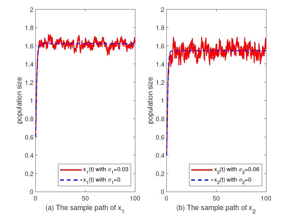
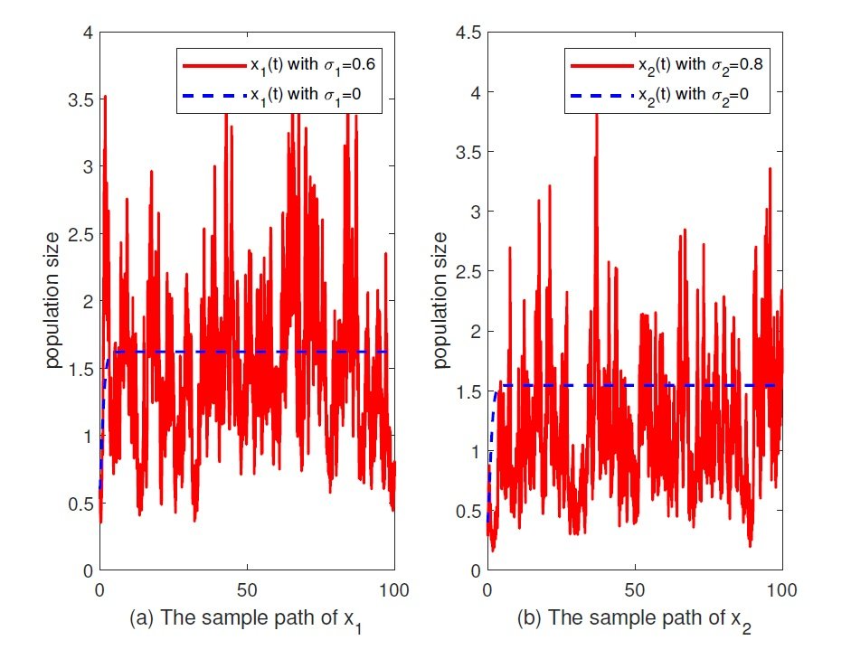
In Figure 1, we take \(\sigma_1=0.03\), \(\sigma_2=0.06\), then the solution of system (2) fluctuate around \(E_0\) with a small amplitude, while we choose \(\sigma_1=0.5\), \(\sigma_2=0.6\), then by a simple calculation, \(r_1=1.5>b_2+0.5\sigma^2_1=0.6+0.5\times0.25=0.725\), \(r_2=1.7>b_1+0.5\sigma^2_2=0.5+0.5\times0.36=0.68\), the solution of system (2) fluctuate around \(E_0\) with a big range in Figure 2. So a small environment noise could not disrupt the permanence, and the population density will neither too small nor too large with probability one when the time is sufficiently large.
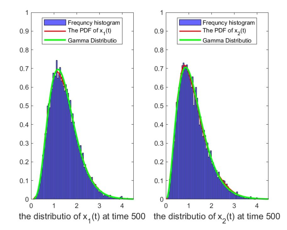
Let \(\sigma_1=0.5,\ \sigma_2=0.6\), then by a simple calculation, the assumptions of Theorem 6 are hold, and then system (47) has a unique stationary distribution. To verify this result, we perform a computer simulation of \(10^4\) iterations of the sample trajectory of \(x_1(t)\) and \(x_2(t)\). By utilizing the method of kernel density estimator, we present the probability density function of \(x_1\) and \(x_2\) at time \(t=500\). To understand the distribution type of \(x_1(t)\) and \(x_2(t)\), we simulated \(10^4\) sample paths, and fitted the data at time \(t=500\) with a gamma distribution. The red line represents the probability density curve of \(x_1\) and \(x_2\), the other one represents the probability density curve of gamma distribution, and it seems to achieved a good fit, see Figure 3.
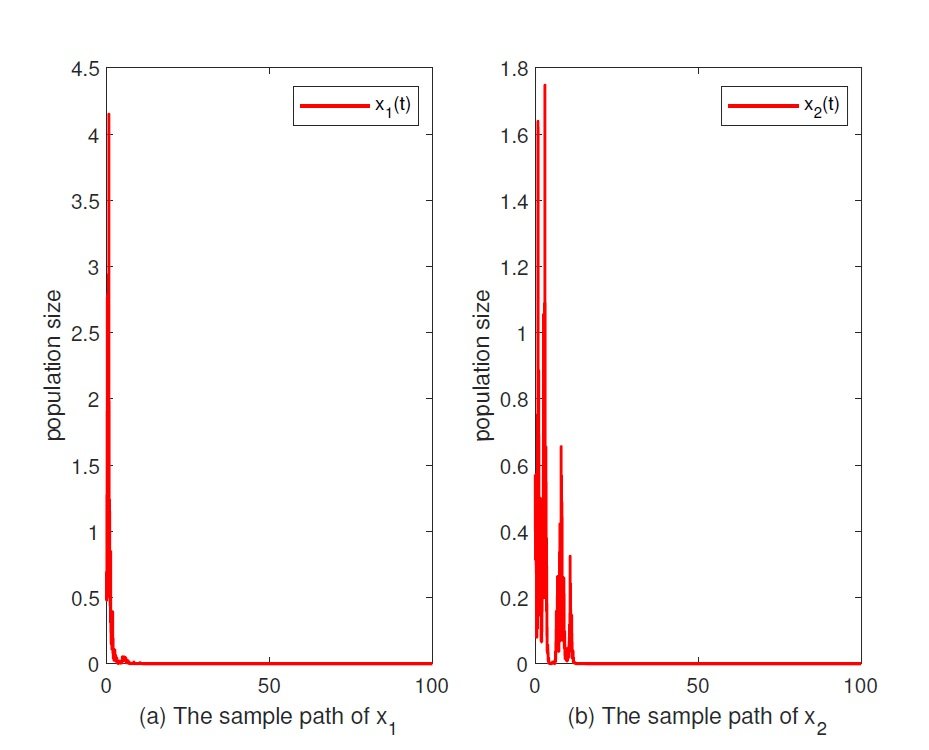
Example 2. The conclusion (2) in Theorem 5 shows that a large environment noise will force the species incline to extinction with probability one. Let \(\sigma_1=2, \sigma_2=2.1\), then we compute that \(r_1=1.5<0.5\sigma^2_1=0.5\times4=2\), \(r_2=1.7<0.5\sigma^2_2=0.5\times4.41=2.205\), then population \(x_i\) tend to be extinction almost surely, see Figure 4.
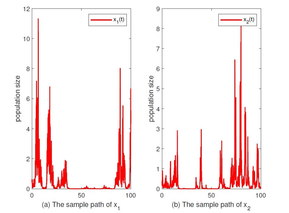
Example 3. The conclusion (3) in Theorem 5 admits the case that population size is close to zero even the time is sufficiently large, that is to say, the survival of species could be dangerous in reality. Let \(\sigma_1=1.5, \sigma_2=1.7\), by a straightforward calculation, \(r_1=1.5>0.5\sigma^2_1=0.5\times2.25=1.025\), \(r_2=1.7>0.5\sigma^2_2=0.5\times2.89=1.445\), then population \(x_i\) is weakly persistent almost surely, see Figure 5.
In this work, we mainly study the dynamical behaviors of system (2), such as stochastic permanence, the estimation of temporal averages of population density, strongly persistence in the mean, weak persistence as well as the existence and uniqueness of stationary distribution. In addition, our analytical results reveal that the dynamical properties of the competition system (2) depends on the intensities of the stochastic perturbations, that is, a small stochastic perturbation does not alter the permanence of the species, but a large one will force the species to become extinct with probability one. And \(r_i=0.5\sigma^2_i\ (i=1,2)\) is the threshold of weak persistence and extinction.
In this paper, we only especially consider the white noise. However, the competition system is also inevitably perturbed by other environment noises, such as L\(\acute{e}\)vy jump, and the regime-switching is other common random perturbations in the environment. All of these interesting topics associated with system (2) deserve further investigation, and we will study these issues in the near future.