
The aim of this paper is to present alternative measurement tools in normed vector spaces ordered by cones, such as the Hilbert projective metric [1] and the Thompson part metric [2], to study spectral properties of homogeneous operators and the existence of solutions to a class of non-homogeneous operator equations. Let \(\mathrm{E}\) be normed vector space and \(\theta\) its zero element. A nonempty closed subset \(\mathrm{K}\) of \(\mathrm{E}\) is called cone if it satisfies three conditions: (i) \(\mathrm{K}+\mathrm{K}=\mathrm{K}\); (ii) \(\lambda\,\mathrm{K}\subseteq \mathrm{K}\) for all \(\lambda>0\); (iii) \(\mathrm{K}\cap(-\mathrm{K})=\{\theta\}\). Let \(\mathrm{K}^{\ast}:= \mathrm{K}\setminus\{\theta\}\) and a nonempty interior of \(\mathrm{K}\) is denoted \(\mathring{\mathrm{K}}\). The notation \(x\le y\) means that \(y-x\in \mathrm{K}\). Two elements \(x,y\in\mathrm{K}^{\ast}\) are said comparable and denoted \(x\sim y\) if there exist real numbers \(\alpha,\beta>0\) such that \(\alpha x \le y \le \beta x\), which is indeed an equivalence relation. Hilbert’s projective metric is defined on \(\mathrm{K}^{\ast}\) by: \[d_{H}(x,y)=\ln\frac{M ({x}/{y} )}{m ({x}/{y} )},\text{ if }x\sim y,\] where \(m ({x}/{y} ):= \sup\{\lambda \colon \lambda x\le y\}\) and \(M ({x}/{y} ):= \inf\{\lambda\colon x\le \lambda y\}\), and \(d_{H}(x,y)=\infty\) if \(x\) and \(y\) are not comparable.
The importance of this projective metric was highlighted by Birkhoff [3], when he provided an elegant proof involving the Hilbert’s projective metric, and showed the existence of a positive eigenvector via the Banach contraction principle. Note that the measure of the distance between two points of the same ray via the Hilbert projective metric is null. This measure is non-null if we use another variant of distance, which was introduced by Thompson, \[d_{T}(x,y)=\ln (M ({x}/{y} )\vee M ({y}/{x} )),\text{ if }x\sim y,\] and \(d_{T}(x,y)=\infty\) if \(x\) and \(y\) are not comparable. Thompson’s distance function is indeed a genuine metric on each part of the cone, where a part is a class of equivalence.
Both Hilbert and Thompson distance functions play important roles in solving linear and nonlinear operator equations. For instance, Hilbert’s projective metric has been applied by Potter [4] to study a class of Hammerstein integral equations. It was also used by Eveson [5] to prove the existence of a positive eigenvector associated with a positive eigenvalue for a linear operator. Hilbert’s projective metric even arises in more complicated systems, as shown by Huang et al. [6] when studying a nonlinear elliptic problem or Reeb et al. [7] in their work on quantum information theory. However, Thompson’s part metric is very effective to solve nonlinear matrix equations as it is shown by Liao et al. [8]. Furthermore, it has been used by Chen [9] and Herzog and Kunstmann [10] to study the stability of difference equations and semilinear equations, respectively. Alternative distance functions, to the Thompson metric, have been introduced by the author in [11]. Here we show how to construct projective suprametrics and part suprametrics connected to Hilbert and Thompson distance functions.
In this paper, we introduce the concept of projective suprametrics and provide new part suprametrics in normed vector spaces. We present their interconnections and mutual relations with the Hilbert and Thompson distance functions, and furnish various examples. We study the link between the different notions of convergences. As a byproduct, we get new inequalities for Hilbert’s and Thompson’s distances. We provide some sufficient conditions for the completeness of certain subsets of the space. We prove a theorem of Krein-Rutman for strongly positive operators via some existing fixed point theorems and involving projective suprametrics. We further establish a Geraghty fixed point theorem in suprametric spaces and show that certain classes of concave or convex operators satisfy the contraction of Geraghty type. As an application, we prove a Perron-Frobenius theorem and show the existence of positive eigenvalue and eigenvector to a tensor spectral problem.
The paper is organized as follows: §2 presents the pseudo-suprametric spaces. §3 introduces some projective and genuine suprametrics. The convergence relationships are investigated in §4. §5 presents some conditions for the completeness. In §6, we establish a new fixed point theorem of Geraghty type. §7 presents some theorems of Krein-Rutman types. In §8, we study certain concave and convex operators. §9 is devoted to the investigation of a problem of tensor eigenvalues.
In this section, we present the concept of pseudo-suprametric and provide an example of bounded suprametric.
Definition 1. Let \(X\) be a nonempty set and \(\rho\) be a constant in \([0,+\infty)\). Let \(d\colon X\times X \to [0,+\infty)\) be a function and for all \(x,y,z\in X\) consider the following properties:
(d1) \(d(x,y)=0 \implies x=y\).
(d2) \(d(x,x)=0\).
(d3) \(d(x,y)=d(y,x)\).
(d4) \(d(x,y)\le d(x,z)+d(z,y)+ \rho \,d(x,z)d(z,y)\).
A pair \((X,d)\) is called suprametric space if \(X\) is a nonempty set and \(d\) satisfies (d1)–(d4), and it is called pseudo-suprametric space if \(X\) is a nonempty set and \(d\) satisfies (d1)–(d4).
For examples of suprametrics, we refer the reader to [11]. We next provide an example of a suprametric whose range is \([0,1)\).
Example 1. Let \(X=\mathbb{R}\) and \(d\colon X\times X \to [0,1)\) be the function given by \[d(x,y)=1-e^{-|x-y|(|x-y|+1)},\;\text{ for all } x,y\in X.\]
Then \(d\) is a suprametric for \(\rho=1\). Precisely, (d1)–(d3) hold easily and (d4) comes from the following technical lemma.
Lemma 1. For all \(s,t\ge 0\), \(e^{s}+e^{t}\le e^{s+t}+e^{-st}\).
Proof. Firstly, observe that if \(s=0\) or \(t=0\) the inequality becomes equality. We now show that the inequality holds for \(t=s>0\), that is, \[2e^{s}\le e^{2s}+e^{-s^2},\; s> 0.\]
By the monotonicity of the function \(s\mapsto e^{s}+e^{-s-s^{2}}-2\), we deduce that it is positive for \(s>0\), which implies that \(e^{s}-1\ge 1-e^{-s-s^{2}}=\left(e^{s}-e^{-s^{2}}\right)e^{-s}\) or equivalently \(e^{s}\left(e^{s}-1\right)+e^{-s^2}\ge e^{s}\).
Without loss of generality, suppose now that \(s>t>0\). If \(t\ge 1\), then by the mean value theorem, it follows that there exists a constant \(c\in(0,t)\) such that \(e^{s}\left(e^{t}-1\right)+e^{-st}= te^{s+c}+e^{-st}\ge e^{t}\). Otherwise, if \(t<1\), we will instead prove the following equivalent inequality \[\begin{aligned} e^{st+t}-1 \le e^{st+s+t}-e^{st+s}. \end{aligned}\]
To this end, we apply twice [12, Lemma 2] (see also [13]), which asserts that for all \(x,y\in\mathbb{R}\) such that \(x\ne y\), we have \[e^{\frac{x+y}{2}}\le \frac{e^{x}-e^{y}}{x-y} \le \frac{1}{2}\left(e^{x}+e^{y}\right).\]
Hence, since \(st+t\ne0\) and \(st+s+t\ne st+s\), we get \[e^{st+t}-1 \le \frac{1}{2}(st+t)\left(e^{st+t}+1\right) \;\text{ and }\; te^{st+s+\frac{t}{2}}\le e^{st+s+t}-e^{st+s}.\]
We claim that \(\frac{1}{2}(st+t)(e^{st+t}+1)\le te^{st+s+\frac{t}{2}}\) if \(0<t<s\) with \(t<1\). Observe first that if \(t\in\left(0,1\right)\), \(\left(t+\ln{\left(\frac{1-t}{1+t}\right)}\right)'=\frac{t^{2}+1}{{\mathstrut}t^{2}-1}<0\), we deduce that \(2t+2\ln{\left(\frac{1-t}{1+t}\right)}<0\) or equivalently \(\left(1-t\right)^{2}e^{t}<\left(1+t\right)^{2}e^{-t}\) thus \(t\mapsto \frac{e^{t}}{1+t}-\cosh{\frac{t}{{\mathstrut}2}}\) is increasing on \(\left(0,1\right)\) since \(\left(\frac{e^{t}}{1+t}-\cosh{\frac{t}{2}}\right)'=\frac{1}{{\mathstrut}4\left(1+t\right)^{2}}\left(\left(1+t\right)^{2}e^{-t}-\left(1-t\right)^{2}e^{t}\right)+\frac{1}{2}\left(\sinh{t}-\sinh{\frac{t}{2}}\right)\), which implies that \(\frac{e^{t}}{t+1}\ge\cosh{\frac{t}{{\mathstrut}2}}\), so by monotonicity of \(t\mapsto \frac{e^{t}}{1+t}\) we deduce for \(s>t\) that \[\frac{e^{s}}{1+s}\ge\frac{e^{t}}{1+t}\ge \frac{1}{2}\left(e^{\scriptstyle\frac{t}{{\mathstrut}2}}+e^{-\scriptstyle\frac{t}{{\mathstrut}2}}\right)\ge \frac{1}{2}\left(e^{\scriptstyle\frac{t}{{\mathstrut}2}}+e^{-st-\scriptstyle\frac{t}{{\mathstrut}2}}\right).\]
Hence, our claim follows easily from the following inequality \[e^{st+\frac{t}{2}}e^{s}\ge {\frac{1}{2}}e^{st+\frac{t}{2}}\left(1+s\right)\left(e^{\frac{t}{2}}+e^{-st-\frac{t}{2}}\right).\] ◻
Let us now return to the proof of (d4) of Example 1. Note that from [11, Example 1.1], we have that \(\left(x,y\right)\mapsto |x-y|\left(|x-y|+1\right)\) is a suprametric with \(\rho=1\), then we deduce \[d(x,y)\le 1-e^{-s-t-st},\] where \(s=|x-z|\left(|x-z|+1\right)\) and \(t=|z-y|\left(|z-y|+1\right)\). To show (d4) it suffice to show that \[\begin{aligned} 1-e^{-s-t-st}&\le \left(1-e^{-s}\right)+\left(1-e^{-t}\right)+ \left(1-e^{-s}\right)\left(1-e^{-t}\right) \\ &= 3-2e^{-s}-2e^{-t}+e^{-s-t}, \end{aligned}\] or equivalently \[2e^{s+t}-2e^{s}-2e^{t}+e^{-st}+1\ge0,\] which follows easily from the previous lemma. However, it is worthy to note that \(d\) is not a metric, since \(d(x,y)>d(x,z)+d(z,y)\) when \(10z\,{=}\,20x\,{=}\,5y\,{=}\,1\).
At the end of this section recall that the concepts of convergence and completeness are similar to that in metric spaces.
In what follows we will adopt the following notations. Let \(E\) be a real normed vector space and \(\mathrm{K}\) its cone. \(\mathrm{K}\) is called solid if \(\mathring{\mathrm{K}}\) is nonempty. The order interval \([x,y]:= \left(x+K\right)\cap\left(y-K\right)\). The notation \(x< y\) means that \(y-x\in\mathring{\mathrm{K}}\) whenever \(\mathrm{K}\) is solid. Moreover if \(\mathrm{K}\) is solid, an operator \(A\colon E\to E\) is called strictly (strongly) positive if \(A\left(\mathring{\mathrm{K}}\right)\subseteq \mathring{\mathrm{K}}\) (\(A\left(\mathrm{K}^{\ast}\right)\subseteq \mathring{\mathrm{K}}\)). A positive operator \(A\) is said increasing (resp. decreasing) whenever \(Ax\le Ay\) (resp. \(Ax\ge Ay\)) if \(x\le y\). If \(\mathrm{K}\) is solid, a strongly positive operator \(A\) is said strongly increasing whenever \(Ax< Ay\) if \(x\le y\) with \(x\ne y\). A positive operator \(A\) is called \(p\)-homogeneous on \(\mathrm{S}\subseteq \mathrm{K}\) if \(A\left(\lambda x\right)=\lambda^{p}Ax\) for all \(\lambda>0\) and \(x\in \mathrm{S}\), where \(p\in[0,\infty)\) is constant. If \(E\) is equipped with a norm \(\|\cdot\|\), \(\mathrm{K}\) is called normal if there exists a constant of normality \(c_{N}>0\) such that \(x\le y\) implies \(\left\|x\right\|\le c_{N}\left\|y\right\|\). The norm is said to be monotone if \(x\le y\) implies \(\left\|x\right\|\le \left\|y\right\|\). Let \(r\,{>}\,0\), and define the set \(\mathrm{S}_{r}:=\{x\in \mathrm{K}\colon \left\|x\right\|=r\}\) and if \(\mathrm{K}\) is solid, we define the set \(\mathring{\mathrm{S}}_{r}:=\{x\in \mathring{\mathrm{K}}\colon \left\|x\right\|=r\}\). The open ball of center \(z\) and of radius \(r\) is denoted by \(\mathrm{B}\left(z;r\right):=\{x\in E: \left\|x-z\right\|<r\}\). An operator \(A\colon \mathrm{E} \to \mathrm{F}\) is said compact if the image of bounded subsets of \(\mathrm{E}\) are relatively compact subsets of \(\mathrm{F}\). Now we recall a result of Bushell [14].
Lemma 2. If \(x,y\in \mathrm{K}^{\ast}\) and \(M ({x}/{y} )\) is finite, then \(m ({x}/{y} ) y\le x \le M ({x}/{y} ) y\). Moreover, \(0< m ({x}/{y} )\le M ({x}/{y} )<\infty\) for all \(x,y\in\mathring{\mathrm{K}}\) when \(\mathrm{K}\) is solid.
In the sequel, if \(\mathrm{K}\) is solid, then for all \(x,y,z\in\mathring{\mathrm{K}}\) and all \(\lambda,\mu>0\), we have \[ m ({x}/{z} )m ({z}/{y} ) \le m ({x}/{y} ),\;\;M ({x}/{y} )\le M ({x}/{z} )M ({z}/{y} ).\label{e1}\ \tag{1}\] \[m ({\lambda x}/{\mu y} )=\frac{\lambda}{\mu}m ({x}/{y} ),\; \;M ({\lambda x}/{\mu y} )=\frac{\lambda}{\mu}M ({x}/{y} ).\ \tag{2}\] \[m ({x}/{y} )M ({y}/{x} )=1. \tag{3}\] More properties are presented in [15, 16]. From now on, we fix the constants \(\kappa\in [1,+\infty)\) and \(\tau\in [2,+\infty)\), and for all \(x,y\in\mathring{\mathrm{K}}\), we define \[\begin{aligned} \pi_{m}({x,y})&:=\left(m ({x}/{y} )m ({y}/{x} )\right)^{\kappa}, &\pi_{M}({x,y})&:=\left(M ({x}/{y} )M ({y}/{x} )\right)^{\kappa},\\ {\varLambda}({x,y})&:=\left(m ({x}/{y} )\wedge m ({y}/{x} )\right)^{\tau}, &{V}({x,y})&:=\left(M ({x}/{y} )\vee M ({y}/{x} )\right)^{\tau}. \end{aligned}\]
Remark that for all \(x,y\in\mathring{\mathrm{K}}\), by (3) we have \[\label{rel} \pi_{m}({x,y})=\pi_{M}({x,y})^{-1}\,\text{ and }\;{\varLambda}({x,y})={V}({x,y})^{-1}. \tag{4}\]
If the norm is monotone, then for all \(x,y\,{ \in }\,\mathring{\mathrm{K}}\) it follows from Lemma 2 that \[\label{ppm} 0<\pi_{m}({x,y})\le m ({x}/{y} )\le 1 \le M ({x}/{y} )\le\pi_{M}({x,y}). \tag{5}\] For all \(x,y\in\mathring{\mathrm{K}}\), we easily obtain:
(p1) \(\pi_{m}({x,y})x\le m ({x}/{y} )m ({y}/{x} )x\le m ({x}/{y} )y\le{x}\).
(p2) \(x\le M ({x}/{y} ) y \le M ({x}/{y} ) M ({y}/{x} )x\le \pi_{M}({x,y})x\).
(p3) \({\varLambda}({x,y})x\le m ({x}/{y} )m ({y}/{x} )x\le m ({x}/{y} )y\le{x}\).
(p4) \(x\le M ({x}/{y} ) y \le M ({x}/{y} ) M ({y}/{x} )x\le {V}({x,y}) x\).
(p5) \({\varLambda}({x,y})y\le \left(m ({x}/{y} )\wedge m ({y}/{x} )\right)y\le m ({x}/{y} )y\le{x}\).
(p6) \(x\le M ({x}/{y} ) y \le \left(M ({x}/{y} )\vee M ({y}/{x} )\right)y\le {V}({x,y}) y\).
(p7) \(\pi_{m}({x,y})\le m ({x}/{y} )m ({y}/{x} )\le 1 \le M ({x}/{y} ) M ({y}/{x} )\le\pi_{M}({x,y})\).
(p8) \({\varLambda}({x,y})\le m ({x}/{y} )m ({y}/{x} )\le 1 \le M ({x}/{y} ) M ({y}/{x} )\le {V}({x,y})\).
(p9) \({\varLambda}({x,y})\le m ({x}/{y} )\le M ({x}/{y} )\le {V}({x,y})\).
Definition 2. Let \(d_{m}\colon \mathrm{K}^{\ast}\,{ \times }\, \mathrm{K}^{\ast} \to [0,1]\) be given by, \[d_{m}(x,y)=\left \{\begin{array}{ll} 1-\pi_{m}({x,y}),& \text{if }x\sim y, \\ 1,& \text{otherwise}. \end{array} \right.\]
Let \(d_{M}\colon \mathrm{K}^{\ast}\,{ \times }\, \mathrm{K}^{\ast}\to [0,\infty]\) be given by, \[d_{M}(x,y)=\left \{\begin{array}{ll} \pi_{M}({x,y})-1,& \text{if }x\sim y, \\ \infty,& \text{otherwise}. \end{array} \right.\]
The next proposition justifies the projective nomenclature of \(d_{m}\) and \(d_{M}\).
Proposition 1. Let \(\mathrm{K}\) be a solid cone. If \(d\) is either \(d_{m}\) or \(d_{M}\) then
(i) \(d(\lambda x,\mu y)=d(x,y)\) for all \(x,y\in\mathring{\mathrm{K}}\) and \(\lambda,\mu>0\).
(ii) \(d(x,y)=0\) for \(x,y\in\mathring{\mathrm{K}}\), then \(x=\lambda y\) for all \(\lambda>0\).
Proof. From (2) follows immediately (i), and (ii) follows easily from Lemma 2, (i), (3), (p1), (p2) and the respective definition of \(d\). ◻
Next, we show that a subset of \(\mathrm{K}\) endowed with one of the projective suprametrics is a suprametric space.
Theorem 1. Let \(\mathrm{K}\) be a solid cone. If \(d\) is equal to \(d_{m}\) or \(d_{M}\), then \((\mathring{\mathrm{K}},d)\) is a pseudo-suprametric space and \((\mathring{\mathrm{S}}_{r},d)\) is a suprametric space.
Proof. Clearly, (d1) does not holds because of Proposition 1 except if \(x,y\in \mathring{\mathrm{S}}_{r}\), however (d2) and (d3) follow from the very definition of \(d\). We now show that (d4) is satisfied for both \(d_{m}\) and \(d_{M}\). By (1) and (p7), we have \[\begin{aligned} d_{m}(x,y) \le&\; 1-(m ({x}/{z} )m ({z}/{y} ) m ({y}/{z} )m ({z}/{x} ))^{\kappa}\\ \le&\; 1-\pi_{m}({x,z})\pi_{m}({z,y}) +2(1-\pi_{m}({x,z}))(1-\pi_{m}({z,y}))\\ =&\; 3- 2\pi_{m}({x,z})- 2\pi_{m}({z,y}) + \pi_{m}({x,z}) \pi_{m}({z,y})\\ =&\; d_{m}(x,z)+d_{m}(y,z)+d_{m}(x,z)d_{m}(y,z).\\[2mm] d_{M}(x,y) \le&\; (M ({x}/{z} )M ({z}/{y} )M ({y}/{z} )M ({z}/{x} ))^{\kappa}-1\\ =&\; d_{M}(x,z)+d_{M}(y,z)+d_{M}(x,z) d_{M}(y,z). \end{aligned}\] ◻
Remark 1. Let \(\mathrm{K}\) be a solid cone. It is worthy to note that on \(\mathring{\mathrm{K}}\) and by (4), we have \[d_{m}=\tfrac{ d_{M}}{ 1+d_{M}} \;\text{ and }\; d_{M}=\tfrac{ d_{m}}{ 1-d_{m}} .\]
Hilbert’s projective metric is related to \(d_{m}\) and \(d_{M}\) as following: \[\begin{gathered} d_{m}=1-e^{-\kappa d_{H}},\quad d_{M}=e^{\kappa d_{H}}-1,\\ d_{H}=-\kappa^{-1}\ln(1-d_{m}),\quad d_{H}=\kappa^{-1}\ln(d_{M}+1). \end{gathered}\]
Next we give examples of projective suprametrics.
Example 2. Let \(\mathrm{E}:=\mathbb{R}^{n}\), \(\mathrm{K}:=\{(x_{1},\ldots,x_{n}): x_{i}\ge 0, 1\le i \le n\}\) and \(\mathring{\mathrm{K}}= \{(x_{1},\ldots,x_{n}): x_{i}> 0, 1\le i \le n\}\). By using \(m ({x}/{y} )=\min_{1\le{i}\le{n}}\frac{x_{i}}{y_{i}}\) and \(M ({x}/{y} )=\max_{1\le{i}\le{n}}\frac{x_{i}}{y_{i}}\), we define the functions \(d_{m}\colon \mathring{\mathrm{K}}\times \mathring{\mathrm{K}}\to [0,1)\) and \(d_{M}\colon \mathring{\mathrm{K}}\times \mathring{\mathrm{K}}\to [0,+\infty)\) by: \[d_{m}(x,y)=1- \left(\min\limits_{1\le{i},{j}\le{n}}\frac{x_{i}y_{j}}{y_{i}x_{j}}\right)^{\kappa}\quad\text{ and }\quad d_{M}(x,y)=\left(\max\limits_{1\le{i},{j}\le{n}}\frac{x_{i}y_{j}}{y_{i}x_{j}}\right)^{\kappa}-1.\]
Example 3. Let \(\mathrm{E}:= C[0,1]\) be a space of all real-valued continuous functions defined on \([0,1]\). Let \(\mathrm{K}:=\{x\in \mathrm{E}: x(t)\ge 0, 0\le t\le 1\}\) and \(\mathring{\mathrm{K}}:=\{x\in \mathrm{E}: x(t)> 0, 0\le t\le 1\}\). For all \(x,y\in\mathring{\mathrm{K}}\), we use \(m ({x}/{y} )=\inf_{t\in[0,1]}\tfrac{ x(t)}{ y(t)}\) and \(M ({x}/{y} )=\sup_{t\in[0,1]}\tfrac{ x(t)}{ y(t)}\), we then define the functions \(d_{m}\colon \mathring{\mathrm{K}}\times \mathring{\mathrm{K}}\to [0,1)\) and \(d_{M}\colon \mathring{\mathrm{K}}\times \mathring{\mathrm{K}}\to [0,+\infty)\) by: \[d_{m}(x,y)=1-\left(\inf\limits_{s,t\in[0,1]}\tfrac{ x(s)y(t)}{ y(s)x(t)} \right)^{\kappa}\quad\text{and}\quad d_{M}(x,y)=\left(\sup\limits_{s,t\in[0,1]}\tfrac{ x(s)y(t)}{ y(s)x(t)} \right)^{\kappa}-1.\]
Example 4. Let \(E\) be the set of positive definite matrices, \(\mathrm{K}(n)\) be the cone of positive semi-definite matrices of size \(n\) and \(\mathring{\mathrm{K}}(n)\) its interior. If we denote by \(\lambda_{M}(S)\) and \(\lambda_{m}(S)\) respectively the greatest and the least eigenvalue of any matrix \(S\in \mathring{\mathrm{K}}(n)\), so as in [17, Lemma 2.1] (see also [18]), then we define \(d_{m}\colon \mathring{\mathrm{K}}(n){\times} \mathring{\mathrm{K}}(n) \to [0,1)\) and \(d_{M}\colon \mathring{\mathrm{K}}(n){\times} \mathring{\mathrm{K}}(n) \to [0,+\infty)\) by \[d_{m}(A,B)=1-\lambda_{m}(A^{-1}B)^{\kappa}\lambda_{m}(B^{-1}A)^{\kappa}\quad\text{and}\quad d_{M}(A,B)=\lambda_{M}(A^{-1}B)^{\kappa}\lambda_{M}(B^{-1}A)^{\kappa}-1.\]
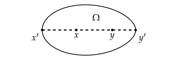
Example 5. Let \((E,\|\cdot\|)\) be a real \((n+1)\)-dimensional affine normed space. Let \(\mathrm{K}\subset \mathrm{E}\) be a solid a cone and \(\mathrm{H}\subset \mathrm{E}\) be an \(n\)-dimensional affine hyperplane such that \(\Omega:= \mathrm{H}\cap \mathring{\mathrm{K}}\) is open, bounded, convex set. The line joining two distinct points \(x\) and \(y\) of \(\Omega\) intersects \(\partial \Omega\) in \(x'\) and \(y'\) such that \(x\) is between \(x'\) and \(y\), and \(y\) is between \(x\) and \(y'\) (cf. Figure 1).
Define the functions \(\delta_{m}\colon \Omega\times \Omega\to [0,1)\) and \(\delta_{M}\colon \Omega\times \Omega\to [0,+\infty)\) by \[\begin{gathered} \delta_{m}(x,y)=1-\left(\frac{\|x-x'\|\|y-y'\|}{\|y-x'\|\|x-y'\|}\right)^{\kappa}\;\text{ and }\; \delta_{M}(x,y)=\left (\frac{\|y-x'\|\|x-y'\|}{\|x-x'\|\|y-y'\|}\right )^{\kappa}-1, \end{gathered}\] for all \(x\ne y\) in \(\Omega\), and \(\delta(x,x)=0\) for all \(x\in\Omega\). Then using the same arguments as that of the proof of [19, Theorem 2.2], we get \[M ({x}/{y} )=\frac{\|x-y'\|}{\|y-y'\|}\;\text{ and }\; M ({y}/{x} )=\frac{\|y-x'\|}{\|x-x'\|},\] and the restriction of \(d_{m}\) and \(d_{M}\) to \(\Omega\) coincide respectively with \(\delta_{m}\) and \(\delta_{M}\).
We next present new part suprametrics.
Definition 3. Let \(d_{\varLambda}\colon \mathrm{K}^{\ast}\times \mathrm{K}^{\ast}\to [0,1]\) be given by \[d_{\varLambda}(x,y)=\left \{\begin{array}{ll} 1-{\varLambda}({x,y}),& \text{if }x\sim y, \\ 1,& \text{otherwise}. \end{array} \right.\]
Let \(d_{V}\colon \mathrm{K}^{\ast}\times\mathrm{K}^{\ast}\to [0,+\infty]\) be given by \[d_{V}(x,y)=\left \{\begin{array}{ll} {V}({x,y})-1,& \text{if }x\sim y, \\ \infty,& \text{otherwise}. \end{array} \right.\]
We need the following obvious lemma in the proof of suprametrics.
Lemma 3. \((ab\wedge cd)\ge(a\wedge c)(b\wedge d)\) and \((ab \vee cd)\le(a\vee c)(b\vee d)\), for all \(a,b,c,d\in[0,+\infty).\)
Theorem 2. Let \(\mathrm{K}\) be a solid cone. If \(d\) is either \(d_{\varLambda}\) or \(d_{V}\), then \((\mathring{\mathrm{K}},d)\) is a suprametric space.
Proof. If \(d\,{ = }\,d_{\varLambda}\), then \(d_{\varLambda}(x,y)\,{ = }\,0\) implies that \({\varLambda}({x,y})\,{ = }\,1\). Without loss of generality, we assume that \(m ({x}/{y} )\,{ = }\,1\), so by (p9) and (4) it follows that \(m ({y}/{x} )\,{=}\,1\), which implies that \(x\,{ = }\,y\) and (d1) holds. Similarly, if \(d\,{ = }\,d_{V}\) we get \(d_{V}(x,y)\,{ = }\,0\) implies \(x=y\) and again (d1) holds. Now, (d2) and (d3) follows immediately from the definition of \(d\). We next show that (d4) is satisfied for \(d_{\varLambda}\) and \(d_{V}\). By using (1), (p3), (p4) and Lemma (3), we obtain \[\begin{aligned} d_{\varLambda}(x,y) &\le 1-(m ({x}/{z} )m ({z}/{y} )\wedge m ({y}/{z} )m ({z}/{x} ))^{\tau}\\ &\le 1-{\varLambda}({x,z}){\varLambda}({z,y}) +2(1-{\varLambda}({x,z}))(1-{\varLambda}({z,y}))\\ &= 3-2\, {\varLambda}({x,z}) – 2\, {\varLambda}({z,y}) + {\varLambda}({x,z}) {\varLambda}({z,y})\\ &= d_{\varLambda}(x,z)+d_{\varLambda}(y,z)+d_{\varLambda}(x,z)d_{\varLambda}(y,z).\\[2mm] d_{V}(x,y) &\le (M ({x}/{z} )M ({z}/{y} )\vee M ({y}/{z} )M ({z}/{x} ))^{\tau}-1\\ &\le {V}({x,z}){V}({z,y})-1\\ &= d_{V}(x,z)+d_{V}(y,z)+d_{V}(x,z) d_{V}(y,z). \end{aligned}\] ◻
Remark 2. Let \(\mathrm{K}\) be a solid cone. It is worthy to note that on \(\mathring{\mathrm{K}}\) and by (4), we have \[d_{\varLambda}=\frac{d_{V}}{1+d_{V}}\;\text{ and }\; d_{V}=\frac{d_{\varLambda}}{1-d_{\varLambda}}.\]
Thompson’s metric \(d_{T}\) is related to \(d_{\varLambda}\) and \(d_{V}\) as following: \[\begin{gathered} d_{\varLambda}=1-e^{-\tau d_{T}},\quad d_{V}=e^{\tau d_{T}}-1,\\ d_{T}=-\tau^{-1}\ln(1-d_{\varLambda}),\quad d_{T}=\tau^{-1}\ln(d_{V}+1). \end{gathered}\]
Example 6. Under the hypotheses of Example 2, we define the functions \(d_{\varLambda}\colon \mathring{\mathrm{K}}\times \mathring{\mathrm{K}}\to [0,1)\) and \(d_{V}\colon \mathring{\mathrm{K}}\times \mathring{\mathrm{K}}\to [0,+\infty)\) by: \[d_{\varLambda}(x,y)=1- \left(\min_{1\le{i}\le{n}}\left(\frac{x_{i}}{y_{i}}\right)\wedge\min_{1\le{i}\le{n}}\left(\frac{y_{i}}{x_{i}}\right)\right)^{\tau}\quad\text{and}\quad d_{V}(x,y)=\left(\max_{1\le{i}\le{n}}\left(\frac{x_{i}}{y_{i}}\right)\vee\max_{1\le{i}\le{n}}\left(\frac{y_{i}}{x_{i}}\right)\right)^{\tau}-1.\]
Example 7. Under the hypotheses of Example 3, we define the functions \(d_{\varLambda}\colon \mathring{\mathrm{K}}\times \mathring{\mathrm{K}}\to [0,1)\) and \(d_{V}\colon \mathring{\mathrm{K}}\times \mathring{\mathrm{K}}\to [0,+\infty)\) by: \[d_{\varLambda}(x,y)=1-\left(\inf\limits_{t\in[0,1]}\tfrac{ x(t)}{ y(t)} \wedge\inf\limits_{t\in[0,1]}\tfrac{ y(t)}{ x(t)} \right)^{\tau} \quad\text{and}\quad d_{V}(x,y)=\left(\sup\limits_{t\in[0,1]}\tfrac{ x(t)}{ y(t)} \vee\sup\limits_{t\in[0,1]}\tfrac{ y(t)}{ x(t)} \right)^{\tau}-1.\]
Example 8. Under the hypotheses of Example 4, we define the functions \(d_{\varLambda}\colon \mathring{\mathrm{K}}\times \mathring{\mathrm{K}}\to [0,1)\) and \(d_{V}\colon \mathring{\mathrm{K}}\times \mathring{\mathrm{K}}\to [0,+\infty)\) by: \[d_{\varLambda}(A,B)=1-\left(\lambda_{m}(A^{-1}B)\wedge\lambda_{m}(B^{-1}A)\right)^{\tau}\quad\text{and}\quad d_{V}(A,B)=\left(\lambda_{M}(A^{-1}B)\vee\lambda_{M}(B^{-1}A)\right)^{\tau}-1.\]
Example 9. Under the hypotheses of Example 5, we define the functions \(\delta_{\varLambda}\colon \Omega\times \Omega \to [0,1)\) and \(\delta_{V}\colon \Omega\times \Omega \to [0,+\infty)\) by: \[\delta_{\varLambda}(x,y)=1-\left (\frac{\|y-y'\|}{\|x-y'\|}\wedge\frac{\|x-x'\|}{\|y-x'\|}\right )^{\tau}\quad\text{and}\quad \delta_{V}(x,y)=\left (\frac{\|x-y'\|}{\|y-y'\|}\vee \frac{\|y-x'\|}{\|x-x'\|}\right )^{\tau}-1.\]
The restriction of \(d_{\varLambda}\) and \(d_{V}\) to \(\Omega\) coincide respectively with \(\delta_{\varLambda}\) and \(\delta_{V}\).
In this section we show the links between convergence in suprametrics and that in the underlying norm of vector space.
Proposition 2. Let \(\mathrm{K}\) be a normal solid cone in normed vector space \((\mathrm{E},\|\cdot\|_{1})\) such that \(\|\cdot\|_{1}\) is monotone. Then, for all \(x,y\in \mathring{\mathrm{S}}_{r}\), \[\begin{aligned} \|x-y\|_{1}&\le 2rd_{M}(x,y)=2r\frac{ d_{m}(x,y)}{1-d_{m}(x,y)},\\ \|x-y\|_{1}&\le 2rd_{V}(x,y)=2r\frac{ d_{\varLambda}(x,y)}{1-d_{\varLambda}(x,y)}. \end{aligned}\]
Proof. From Lemma 2 it follows that \[\theta\le x- m ({x}/{y} ) y \le \left(M ({x}/{y} )-m ({x}/{y} )\right) y.\]
Using the normality of \(\mathrm{K}\) and (5), we obtain \[\| x- m ({x}/{y} ) y \|_{1} \le \left(M ({x}/{y} )-m ({x}/{y} )\right) \| y\|_{1} = r(M ({x}/{y} )-m ({x}/{y} )).\]
Using (5), (p1) and Remark 1, we deduce \[\begin{aligned} \|x-y\|_{1} &\le \| x-m ({x}/{y} ) y\|_{1}+\|(m ({x}/{y} )-1)y\|_{1}\\ &\le r\left(M ({x}/{y} )-m ({x}/{y} )\right)+ r \left(1-m ({x}/{y} )\right) \\ &\le 2 r \left(M ({x}/{y} )-m ({x}/{y} )\right)\\ &\le 2 r \,m ({x}/{y} )\left(M ({x}/{y} )M ({y}/{x} )-1\right)\\ &\le 2 r \left(\pi_{M}({x,y})-1\right)\\ &\le 2 r d_{M}(x,y)= 2r\frac{ d_{m}(x,y)}{1-d_{m}(x,y)}, \text{and by (p8), we obtain} \|x-y\|_{1} &\le 2 r \,m ({x}/{y} )\left(M ({x}/{y} )M ({y}/{x} )-1\right)\\ &\le 2 r \left({V}({x,y})-1\right)\\ &\le 2 r d_{V}(x,y)=2r\frac{ d_{\varLambda}(x,y)}{1-d_{\varLambda}(x,y)}. \end{aligned}\] ◻
Proposition 3. Let \(\mathrm{K}\) be a normal solid cone in a normed vector space \((\mathrm{E},\|{\cdot}\|)\). Then, for all \(x\in \mathring{\mathrm{K}}\) and \(y\in\mathring{\mathrm{S}}_{r}\), \[\begin{aligned} \|x-y\|&\le 2c_{N}r\frac{(2+ d_{M}(x,y))d_{M}(x,y)}{1+d_{M}(x,y)}=2c_{N}r\frac{(2-d_{m}(x,y))d_{m}(x,y)}{1-d_{m}(x,y)},\\ \|x-y\|&\le 2c_{N}r\frac{(2+ d_{V}(x,y))d_{V}(x,y)}{1+d_{V}(x,y)}=2c_{N}r\frac{(2-d_{\varLambda}(x,y))d_{\varLambda}(x,y)}{1-d_{\varLambda}(x,y)}. \end{aligned}\]
Proof. From (p7) it follows that \[\begin{aligned} \theta\le x- m ({x}/{y} )m ({y}/{x} ) y &\le \left(M ({x}/{y} )M ({y}/{x} )-m ({x}/{y} )m ({y}/{x} )\right) y. \end{aligned}\]
Hence, by normality of \(\mathrm{K}\), we obtain \[\begin{aligned} \| x- m ({x}/{y} )m ({y}/{x} ) y \| &\le c_{N}\left(M ({x}/{y} )M ({y}/{x} )-m ({x}/{y} )m ({y}/{x} )\right) \| y\|\\ &= c_{N}r\left(M ({x}/{y} )M ({y}/{x} )-m ({x}/{y} )m ({y}/{x} )\right). \end{aligned}\]
Using (5), (p1) and Remark 1, we deduce \[\begin{aligned} \|x-y\| &\le \| x-m ({x}/{y} )m ({y}/{x} ) y\|+\|(m ({x}/{y} )m ({y}/{x} )-1)y\|\\ &\le 2c_{N}r\left(M ({x}/{y} )M ({y}/{x} )-m ({x}/{y} )m ({y}/{x} )\right)\\ &\le 2c_{N}r \left(M ({x}/{y} )M ({y}/{x} )-1\right)+ 2c_{N}r\left(1-m ({x}/{y} )m ({y}/{x} )\right)\\ &\le 2c_{N}r (d_{M}(x,y)+d_{m}(x,y)), \end{aligned}\] and by (p8), we obtain \[\begin{aligned} \|x-y\| &\le 2c_{N}r (d_{V}(x,y)+d_{\varLambda}(x,y)), \end{aligned}\] and the results follows from Remarks 1 and 2. ◻
For \((\kappa,\tau)=(1,2)\) we easily obtain the following inequalities, from the previous proposition and Remarks 1, 2.
Remark 3. For the Hilbert’s projective metric, we have \[\|x-y\|\le 4c_{N}r \sinh{(d_{H}(x,y))}\text{ for all }x\in\mathring{\mathrm{K}}\text{ and }y\in\mathring{\mathrm{S}}_{r}.\]
For the Thompson’s metric, we have \[\|x-y\|\le 4c_{N}r \sinh{(2d_{T}(x,y))}\text{ for all }x\in\mathring{\mathrm{K}}\text{ and }y\in\mathring{\mathrm{S}}_{r}.\]
Some converse inequalities are given in the following proposition.
Proposition 4. Assume \(B(y;r)\subset K\) for some \(y\in \mathring{\mathrm{K}}\). Then, for all \(x\in B(y;r)\), \[\begin{aligned} d_{m}(x,y)&\le 1-\left( \frac{r-\|x-y\|}{r+\|x-y\|}\right)^\kappa, &d_{M}(x,y)&\le \left( \frac{r+\|x-y\|}{r-\|x-y\|}\right)^\kappa-1, \\ d_{\varLambda}(x,y)&\le 1- \left (\frac{r}{r+\|y-x\|}\right )^{\tau}, &d_{V}(x,y)&\le \left (\frac{r}{r-\|y-x\|}\right )^{\tau}-1. \end{aligned}\]
Proof. Following the proof [16, (1.21)], we obtain \(m ({y}/{x} )\ge \frac{r}{r+\|y-x\|}\) and \(M ({y}/{x} )\le \frac{r}{r-\|y-x\|}\), for all \(x\in B(y;r)\) for \(x\,{ \ne }\, y\), which give the desired results. ◻
We next show that equivalence between convergences occur in \(\mathring{\mathrm{S}}_{r}\). We recall first some known facts in the literature. Let \(e\in \mathrm{E}\) such that \(e>\theta\) and \[\mathrm{E}_{e}:=\big\{x\in \mathrm{E} \colon \text{ there exists } \lambda>0 \text{ such that}\, -\lambda e \le x \le \lambda e\big\}.\]
Take a norm \(\|x\|_{e}\) on \(E_{e}\), which is given by \(\|x\|_{e}:=\inf\{\lambda>0 \colon -\lambda e \le x \le \lambda e\}\). Then the pair \((\mathrm{E}_{e},\|\cdot\|_{e})\) is a normed linear space and \(\|\cdot\|_{e}\) is called the \(e\)-norm. It is known [20] that if \(\mathrm{K}\) is normal, then the pair \((\mathrm{E}_{e},\|\cdot\|_{e})\) becomes a Banach space, and there exists a constant \(\omega>0\) such that \(\|x\|\le \omega\|x\|_{e}\). Moreover, \(\mathrm{K}_{e}:= \mathrm{K}\cap \mathrm{E}_{e}\) is a normal solid cone of \(\mathrm{E}_{e}\). If in addition \(\mathrm{K}\) is solid and \(e\in\mathring{\mathrm{K}}\), then \(\mathrm{E}_{e}=\mathrm{E}\) and the \(e\)-norm is equivalent to the norm of \(\mathrm{E}\). In the remainder of this section, we consider that \(\mathrm{K}\) is normal and solid cone.
Proposition 5. Let \(\mathrm{K}\) be a normal solid cone. Let \(x_{\ast}\in\mathring{\mathrm{S}}_{r}\) and \(\{x_{n}\}\subset \mathring{\mathrm{S}}_{r}\). If \(d\) is either \(d_{m}\) or \(d_{M}\), then \[\lim_{n\to\infty}d(x_{n},x_{\ast})=0 \iff \lim_{n\to\infty}\|x_{n}-x_{\ast}\|=0.\]
Proof. We next discuss the cases \(d=d_{m}\) and \(d=d_{M}\).
Case of \(d=d_{m}\).
Let \(x_{\ast}\in\mathring{\mathrm{S}}_{r}\) and \(\{x_{n}\}\subset \mathring{\mathrm{S}}_{r}\), and assume that we have \(\lim_{n\to\infty}d_{m}(x_{n},x_{\ast})=0\). Thus, by definition of \(d_{m}\), \(\lim_{n\to\infty} \pi_{m}({x_{\ast},x_{n}}) =1\), and by (p7) we get \(x_{\ast} \ge m ({x_{\ast}}/{x_{n}} ) m ({x_{n}}/{x_{\ast}} ) x_{n}\ge \pi_{m}({x_{\ast},x_{n}}) x_{\ast}\). Hence, we have \(\theta \le x_{\ast}-m ({x_{\ast}}/{x_{n}} )m ({x_{n}}/{x_{\ast}} ) x_{n} \le (1-\pi_{m}({x_{n},x_{\ast}}))x_{\ast}\), since \(\|x_{\ast}\|=r\), we deduce by the normality of \(\mathrm{K}\) and \(\|x_{n}\|=\|x_{\ast}\|=r\) that we have \(\lim_{n\to\infty} \|m ({x_{\ast}}/{x_{n}} )m ({x_{n}}/{x_{\ast}} ) x_{n}-x_{\ast} \|=0\). Now, by using the triangle inequality, we obtain \[\begin{aligned} \|x_{n}-x_{\ast}\| &\le \big\| x_{n}\,{ – }\,m ({x_{\ast}}/{x_{n}} )m ({x_{n}}/{x_{\ast}} )x_{n}\big\|+\big\|m ({x_{\ast}}/{x_{n}} )m ({x_{n}}/{x_{\ast}} )x_{n}\,{ – }\, x_{\ast}\big\|\\ &\le r(1\,{ – }\,m ({x_{\ast}}/{x_{n}} )m ({x_{n}}/{x_{\ast}} ))+\big\|m ({x_{\ast}}/{x_{n}} )m ({x_{n}}/{x_{\ast}} )x_{n}\,{ – }\,x_{\ast}\big\|\\ &\le 2r(1\,{ – }\,\pi_{m}({x_{\ast},x_{n}})), \end{aligned}\] which tends to zero as \(n\) tends to infinity.
Case of \(d=d_{M}\).
Let \(x_{\ast}\in\mathring{\mathrm{S}}_{r}\) and \(\{x_{n}\}\subset \mathring{\mathrm{S}}_{r}\), and assume that we have \(\lim_{n\to\infty}d_{M}(x_{n},x_{\ast})=0\). So, by definition of \(d_{M}\), \(\lim_{n\to\infty} \pi_{M}({x_{\ast},x_{n}}) =1\), and by (p7) we get \(x_{\ast} \le M ({x_{\ast}}/{x_{n}} )M ({x_{n}}/{x_{\ast}} ) x_{n} \le \pi_{M}({x_{\ast},x_{n}})x_{\ast}\), thus \(\theta \le M ({x_{\ast}}/{x_{n}} )M ({x_{n}}/{x_{\ast}} ) x_{n} \,{ – }\,x_{\ast} \le (\pi_{M}({x_{\ast},x_{n}})\,{ – }\,1)x_{\ast}\). So from the normality of \(\mathrm{K}\) and \(\|x_{n}\|=\|x_{\ast}\|=r\) follows \(\lim\limits_{n\to\infty}\big \|M ({x_{\ast}}/{x_{n}} )M ({x_{n}}/{x_{\ast}} ) x_{n} \,{ – }\,x_{\ast} \big \|\,{ = }\,0\). We conclude that
\[\begin{aligned} \|x_{n}-x_{\ast}\| &\le \big\|x_{n}{ – } M ({x_{\ast}}/{x_{n}} )M ({x_{n}}/{x_{\ast}} )x_{n}\big\|{ + }\big\| M ({x_{\ast}}/{x_{n}} )M ({x_{n}}/{x_{\ast}} )x_{n}{ – }x_{\ast}\big\|\\ &\le r (M ({x_{\ast}}/{x_{n}} )M ({x_{n}}/{x_{\ast}} )\,{ – }\,1) +\big\|M ({x_{\ast}}/{x_{n}} )M ({x_{n}}/{x_{\ast}} )x_{n}\,{ – }\,x_{\ast}\big\|\\ & \le 2r(\pi_{M}({x_{\ast},x_{n}})-1), \end{aligned}\] which tends to zero as \(n\) tends to infinity.
Conversely, assume that \(\lim_{n\to\infty}\|x_{n}-x_{\ast}\|=0.\) Let \(e\in\mathring{\mathrm{K}}\), so \(\mathrm{E}_{e}=\mathrm{E}\) and the \(e\)-norm is equivalent to the norm of \(\mathrm{E}\), which implies that for \(\varepsilon_{n}:=\|x_{n}-x_{\ast}\|_{e}\), we have \(\lim_{n\to\infty}\varepsilon_{n}=0\), and we have \[-\varepsilon_{n} e \le (x_{n}-x) \le \varepsilon_{n} e \;\text{ and }\; -\varepsilon_{n} e \le (x-x_{n}) \le \varepsilon_{n} e.\]
We then take a small real number \(\alpha>0\) such that \(x \ge \alpha e\), since \(x\in \mathring{\mathrm{K}}\). Hence, \[\begin{gathered} (1-\tfrac{ \varepsilon_{n}}{ \alpha} ) x \le x-\varepsilon_{n}e \le x_{n} \le x + \varepsilon_{n}e \le (1+\tfrac{ \varepsilon_{n}}{ \alpha} ) x,\\ (1-\tfrac{ \varepsilon_{n}}{ \alpha} ) x_{n} \le x_{n}-\varepsilon_{n}e \le x \le x_{n} + \varepsilon_{n}e \le (1+\tfrac{ \varepsilon_{n}}{ \alpha} ) x_{n}, \end{gathered}\] which implies that \[\begin{gathered} (1-\tfrac{ \varepsilon_{n}}{ \alpha} )\le m ({x_{n}}/{x} )\le M ({x_{n}}/{x} )\le (1+\tfrac{ \varepsilon_{n}}{ \alpha} ),\\ (1-\tfrac{ \varepsilon_{n}}{ \alpha} )\le m ({x}/{x_{n}} )\le M ({x}/{x_{n}} )\le (1+\tfrac{ \varepsilon_{n}}{ \alpha} ), \end{gathered}\] from which we deduce that \[(1-\tfrac{ \varepsilon_{n}}{ \alpha} )^{2}\le m ({x}/{x_{n}} )m ({x_{n}}/{x} )\;\text{ and }\;M ({x}/{x_{n}} )M ({x_{n}}/{x} )\le (1+\tfrac{ \varepsilon_{n}}{ \alpha} )^{2}.\]
We conclude that \[\begin{gathered} d_{m}(x_{n},x) =1- \pi_{m}({x_{n},x})\le 1-(1-\tfrac{ \varepsilon_{n}}{ \alpha} )^{2\kappa},\\ d_{M}(x_{n},x) = \pi_{M}({x_{n},x})-1 \le (1+\tfrac{ \varepsilon_{n}}{ \beta} )^{2\kappa}-1, \end{gathered}\] and this proves that \(d_{m}(x_{n},x)\) and \(d_{M}(x_{n},x)\) tend to zero as \(n\to \infty\). ◻
Remark 4. Note that Proposition 5 implies that the continuity of an operator on \(\mathring{\mathrm{S}}_{r}\) with respect to the norm or \(d\) are equivalent.
Proposition 6. Let \(x_{\ast}\in\mathring{\mathrm{K}}\) and \(\{x_{n}\}\subset \mathring{\mathrm{K}}\). If \(d\) is either \(d_{m}\) or \(d_{M}\), then \[\lim_{n\to\infty}\|x_{n}-x_{\ast}\|=0 \iff \lim_{n\to\infty}d(x_{n},x_{\ast})=\lim_{n\to\infty}\|x_{n}\|-\|x_{\ast}\|=0.\]
Proof. Assume that \(\lim\limits_{n\to\infty}\|x_{n}-x_{\ast}\|=0\), then clearly \(\lim\limits_{n\to\infty}\|x_{n}\|-\|x_{\ast}\|=0\) and \(\lim_{n\to\infty}\Big \|\frac{x_{n}}{\|x_{n}\|}-\frac{x_{\ast}}{\|x_{\ast}\|}\Big \|=0\). Now, using that \(\frac{rx_{n}}{\|x_{n}\|},\frac{rx_{\ast}}{\|x_{\ast}\|} \in\mathring{\mathrm{S}}_{r}\) it follows from Proposition 5 that \(\lim_{n\to\infty} d\left(\frac{rx_{n}}{\|x_{n}\|},\frac{rx_{\ast}}{\|x_{\ast}\|}\right)=0\) with \(d\) is either \(d_{m}\) or \(d_{M}\). Since \(d\left(\frac{rx_{n}}{\|x_{n}\|},\frac{rx_{\ast}}{\|x_{\ast}\|}\right)=d({x_{n}},{x_{\ast}})\), we conclude that \(\lim_{n\to\infty}d({x_{n}},{x_{\ast}})\,{ = }\,0\).
Conversely, assume that \(\lim_{n\to\infty}d(x_{n},x_{\ast})=\lim_{n\to\infty}\|x_{n}\|-\|x_{\ast}\|=0\), then we get \[\lim_{n\to\infty}d(x_{n},x_{\ast})=\lim_{n\to\infty} d\left(\frac{rx_{n}}{\|x_{n}\|},\frac{rx_{\ast}}{\|x_{\ast}\|}\right)= 0.\]
Using Proposition 5, we get \(\lim_{n\to\infty}\left \|\frac{x_{n}}{\|x_{n}\|}-\frac{x_{\ast}}{\|x_{\ast}\|}\right \|=0\), and by using the triangle inequality of the norm, we obtain
\[\begin{aligned} \|x_{n}-x_{\ast}\| &= \|x_{n}\|\left \| \frac{x_{n}}{\|x_{n}\|}-\frac{x_{\ast}}{\|x_{n}\|}\right \|\\ &\le \|x_{n}\| \left (\left \|\frac{x_{n}}{\|x_{n}\|}-\frac{x_{\ast}}{\|x_{\ast}\|}\right \| +\left \|\frac{x_{\ast}}{\|x_{\ast}\|}-\frac{x_{\ast}}{\|x_{n}\|}\right \|\right ), \end{aligned}\] which tends to zero since \({\|x_{n}\|}\) tends to \({\|x_{\ast}\|}\) as \(n\) tends to infinity. ◻
Proposition 7. Let \(\{x_{n}\}\subset \mathring{\mathrm{K}}\) and \(z\in \mathring{\mathrm{K}}\). If \(d\) is either \(d_{\varLambda}\) or \(d_{V}\), then \[\lim_{n\to \infty}d(x_{n},z)=0 \iff \lim_{n\to \infty}\|x_{n}-z\|=0.\]
Proof. Let \(d\) be either \(d_{\varLambda}\) or \(d_{V}\).
Assume first that \(\lim_{n\to \infty}d(x_{n},z)=0\). Then \(\{x_{n}\}\) is a Cauchy sequence and thus \(\lim_{n,m\to \infty}d(x_{n},x_{m})=0\). As in the proof of Proposition 10, we deduce that there exists \(y\in \mathring{\mathrm{K}}\) such that \(\lim_{n\to \infty}\|x_{n}-y\|=0\) and that \(\lim_{n\to \infty}d(x_{n},y)=0\). Hence, by [11, Proposition 1.4] follows that \(y=z\) and by consequence \(\lim_{n\to \infty}\|x_{n}-y\|=0\).
Conversely, assume that \(\lim_{n\to \infty}\|x_{n}-z\|=0\) and take \(e\in \mathring{\mathrm{K}}\). Then, there exists \(r>0\) such that \(B(e,r):=\{x\in E : \|x-e\|< r\}\subset \mathring{\mathrm{K}}\). As \(z\in \mathring{\mathrm{K}}\) one can choose a sufficiently small number \(\lambda\in(0,r)\) such that \(z\ge\lambda e\). Observe that for \(x\ne z\), we have \(e-\frac{r}{\|x-z\|}(x-z)\in \mathrm{K}\), which implies \(x \le \frac{\|x-z\|}{r}e +z\). Thus, we deduce that \(x_{n} \le (\frac{\|z-x_{n}\|}{\lambda r}+1 )z\), and therefore \[\label{M1} M ({x_{n}}/{z} )\le \frac{\|z-x_{n}\|}{\lambda r}. \tag{6}\]
Moreover, observe that for \(x\ne z\), we have \(e+\frac{r}{\|x-z\|}(x-z)\in \mathrm{K}\), which implies \(z \le \frac{\|x-z\|}{r}e +x\). Next, since there exists an integer \(N\) such that for all \(n\ge N\), \(\|x_{n}-z\|<\lambda\), we obtain \(z \le \left(1-\frac{\|z-x_{n}\|}{\lambda r} \right)^{-1}x_{n}\), so we deduce \[\label{M2} M ({z}/{x_{n}} )\le \left(1-\frac{\|z-x_{n}\|}{\lambda r} \right)^{-1}-1,\;\text{ for all }n>N. \tag{7}\]
Thus from (6) and (7), we conclude that \(\lim_{n\to \infty}d(x_{n},z)=0\), where \(d\) is one of the suprametrics \(d_{\varLambda}\) or \(d_{V}\). ◻
After having shown the link between the convergence in norm and in \(d\) either it is \(d_{m}\) or \(d_{M}\), we present an example highlighting some advantages of the convergence in projective suprametrics.
Example 10. Consider \(\mathrm{E}=C[0,1]\) the set of all continuous real function on \([0,1]\). Let \(\mathrm{K}:=\{f\in E\colon f(t)\ge 0, t\in[0,1]\}\) and \(\mathring{\mathrm{K}}:=\{f\in E\colon f(t)> 0, t\in[0,1]\}\). It is well knows that \(E\) is a Banach space with respect to the norm \(\|\cdot\|\) induced from the distance \(d_{\infty}\), that is, \(\|f-g\|=d_{\infty}(f,g)\) where \[d_{\infty}(f,g)=\sup_{t\in[0,1]}|f(t)-g(t)|.\]
Clearly, \((\mathring{\mathrm{S}}_{r},d_{\infty})\) is not complete. Note that it may occur that \(\lim\limits_{n\to\infty}d_{\infty}(f_{n},f_{\ast})\,{ \ne }\, 0\) while \(\lim\limits_{n\to\infty}d(f_{n},f_{\ast})\,{ = }\,0\) where \(d\) is either \(d_{m}\) or \(d_{M}\). For instance, take \(f_{\ast}(t)\,{ = }\,r\) and \(\{f_{n}\}\) the sequence given by \(f_{n}(t)\,{ = }\,2r\frac{n-t}{n}\), \(t\in[0,1]\). We have \[\lim_{n\to\infty}d_{\infty}(f_{n},f_{\ast})= \lim_{n\to\infty}\sup_{t\in[0,1]} |2r\frac{n-t}{n}-r|\ne 0.\]
Nevertheless, the suprametrics of Example 3 satisfy \[\begin{aligned} &\lim\limits_{n\to\infty}d_{m}(f_{n},f_{\ast}) =\lim\limits_{n\to\infty}d_{m}\left(\frac{1}{2r}f_{n},\frac{1}{r}f_{\ast}\right) = \lim\limits_{n\to\infty} 1-\left( \inf\limits_{s,t\in[0,1]}\frac{n-t}{n-s}\right)^{\kappa}=0,\\ &\lim_{n\to\infty}d_{M}(f_{n},f_{\ast}) =\lim_{n\to\infty}d_{M}\left(\frac{1}{2r}f_{n},{\frac{1}{r}}f_{\ast}\right)= \lim\limits_{n\to\infty} \left( \sup\limits_{s,t\in[0,1]}\frac{n-t}{n-s}\right)^{\kappa}-1=0. \end{aligned}\]
Let \(E\) be a normed vector space. We describe her when completeness holds.
Proposition 8. Let \(\mathrm{K}\) be a normal solid cone in \(\mathrm{E}\) endowed with a monotone norm \(\|\cdot\|_{1}\). If \(d\) is either \(d_{m}\) or \(d_{M}\), \((\mathring{\mathrm{S}}_{r},d)\) is a complete suprametric space.
Proof. Assume that \(\{x_{n}\}\) is a Cauchy sequence in \((\mathring{\mathrm{S}}_{r},d)\). Hence, we have \(\lim_{p,q\to\infty}d(x_{p},x_{q}) =0\). We deduce from (5) that, \[\label{Mm} \lim_{p,q\to\infty}M ({x_{p}}/{x_{q}} )=1 \;\text{ and }\; \lim_{p,q\to\infty}m ({x_{p}}/{x_{q}} ) =1, \tag{8}\] which implies by Proposition 2 that \(\lim_{p,q\to\infty}\|x_{p}-x_{q}\|_{1}=0\), and by completeness of \(\mathrm{E}\) it follows that there exists some \(x_{\ast}\in \mathrm{E}\) such that \(\lim_{n\to\infty}\|x_{n}-x_{\ast}\|_{1} =0\). Note that \(x_{\ast}\in \mathrm{S}_{r}\), so \(\|x_{\ast}\|_{1}=r\).
Assume that \(d=d_{m}\). Thus, for any \(\varepsilon>0\), there is \(\varepsilon_{m}\in(0,1)\) such that \(1- \left( \frac{1-\varepsilon_{m}}{1+\varepsilon_{m}}\right)^{\kappa}<\varepsilon\). By (8), we deduce that there exists \(n_{m}\) such that \[(1-\varepsilon_{m})<m ({x_{p}}/{x_{q}} )\le 1\;\text{ and }\; 1\le M ({x_{p}}/{x_{q}} ) <(1+\varepsilon_{m}),\] for all \(p,q>n_{m}\), thus \(x_{p} \in I_{m}\) where \(I_{m}:=[(1-\varepsilon_{m})x_{q}, (1+\varepsilon_{m})x_{q}]\) for all \(p,q>n_{m}\). Since \(\mathrm{K}\) is closed, then so is the order interval \(I_{m}\), thus by letting \(p\) tends to infinity for a fixed \(q\) in the previous inequality, we obtain \(x_{\ast} \in I_{m}\) for \(q>n_{m}\), which implies \(x_{\ast} \in \mathring{\mathrm{S}}_{r}\) and \[m ({x_{\ast}}/{x_{q}} )\ge (1-\varepsilon_{m}) \;\text{ and }\;M ({x_{\ast}}/{x_{q}} ) \le (1+\varepsilon_{m}),\; q>n_{m}.\]
We conclude that \[d_{m}(x_{\ast},x_{q})=1-\pi_{m}({x_{\ast},x_{q}}) \le1-\left( \frac{1-\varepsilon_{m}}{1+\varepsilon_{m}}\right)^{\kappa}<\varepsilon,\] for \(q>n_{m}\), which proves that \(d_{m}(x_{\ast},x_{q})\) tends to zero as \(q\) tends to infinity.
Assume now that \(d=d_{M}\). Thus, for any \(\varepsilon>0\), there is \(\varepsilon_{M}\in(0,1)\) such that \(\left(\frac{1+\varepsilon_{M}}{1-\varepsilon_{M}} \right)^{\kappa}-1<\varepsilon\). By (8), we deduce that there exists \(n_{M}\) such that \[(1-\varepsilon_{M})<m ({x_{p}}/{x_{q}} )\le 1 \;\text{ and }\;1\le M ({x_{p}}/{x_{q}} ) <(1+\varepsilon_{M}),\] for \(p,q>n_{M}\) thus \(x_{p} \in I_{M}\) where \(I_{M}:=[(1-\varepsilon_{M})x_{q}, (1+\varepsilon_{M})x_{q}]\) for all \(p,q>n_{m}\). By letting \(p\) tends to infinity for a fixed \(q\) in the previous inequality, we obtain \(x_{\ast} \in I_{M}\) for \(q>n_{M}\), so \(x_{\ast} \in \mathring{\mathrm{S}}_{r}\) with \[m ({x_{\ast}}/{x_{q}} )\ge (1-\varepsilon_{M}) \;\text{ and }\; M ({x_{\ast}}/{x_{q}} ) \le (1+\varepsilon_{M}),\; q>n_{M}.\]
We conclude that \[d_{M}(x_{\ast},x_{q})=\pi_{M}({x_{\ast},x_{q}}) -1 \le\left(\frac{1+\varepsilon_{M}}{1-\varepsilon_{M}} \right)^{\kappa}-1<\varepsilon,\] for \(q>n_{M}\), thus \(d_{M}(x_{\ast},x_{q})\) tends to zero as \(q\) tends to infinity. ◻
Proposition 9. Let \(\mathrm{K}\) be a normal solid cone. If \(d\) is either \(d_{m}\) or \(d_{M}\), then \((\mathring{\mathrm{S}}_{r},d)\) is a complete suprametric space.
Proof. Using [21, 1.7 Proposition], there exists a monotone norm denoted \(\|\cdot \|_{1}\) on \(\mathrm{E}\) equivalent to the norm \(\|\cdot \|\). Let \(\mathrm{V}_{r}:=\{x\in \mathring{\mathrm{K}}\colon \|x\|_{1}=r\}\), so it follows by Proposition 8 that \((\mathrm{V}_{1}, d)\) is complete with \(d\) is either \(d_{m}\) or \(d_{M}\). We shall prove that \((\mathring{\mathrm{S}}_{r}, d)\) is complete. Let \(\{x_{n}\}\) be a Cauchy sequence in \((\mathring{\mathrm{S}}_{r}, d)\), so \(\lim_{n,m\to\infty}d(x_{n},x_{m}) =0\). Using that \(\|x_{n}\|=1\) and the equivalence of the norms \(\|\cdot \|\) and \(\|\cdot \|_{1}\), we deduce that there exist two positive real constants \(b\ge a\) such that \(a \|x \| \le \|x \|_{1} \le b \|x \|\), \(x\in \mathrm{E}\). Thus, \(0<a r\le \|x_{n}\|_{1}\le b r\) for all \(n\ge 1\). Take \(z_{n}=\frac{rx_{n}}{\|x_{n}\|_{1}}\), then \(z_{n}\in \mathring{\mathrm{S}}_{r}\) for all \(n\ge 1\). Hence, by Proposition 1, we obtain \[d(z_{p},z_{q})= d\left(\frac{rx_{p}}{\|x_{p}\|_{1}},\frac{rx_{q}}{\|x_{q}\|_{1}}\right)=d(x_{p},x_{q}),\] which tends to zero as \(p,q\) tend to infinity. By virtue of completeness of \((\mathrm{V}_{r}, d)\), there is some \(z_{\ast}\in \mathrm{V}_{r}\) such that \(\lim_{n\to\infty}d(z_{n},z_{\ast}) =0\). Now, since \(\| z_{\ast}\|_{1}=r\) and \(a \|z_{\ast} \| \le \|z_{\ast} \|_{1} \le b \|z_{\ast} \|\), we deduce that \(0<b^{-1}r\le \| z_{\ast}\| \le a^{-1}r\). Now, let \(x_{\ast}=r\frac{z_{\ast}}{\| z_{\ast}\| }\), then \(x_{\ast}\in \mathring{\mathrm{S}}_{r}\) and
\[d(x_{n},x_{\ast})= d\left({\frac{\|x_{n}\|_{1}}{r}z_{n}},\frac{r}{\|z_{\ast}\|_{1}}z_{\ast}\right)=d(z_{n},x_{\ast}),\] which tends to zero as \(n\) tends to infinity, and this implies that \((\mathring{\mathrm{S}}_{r},d)\) is complete, where \(d\) is equal to \(d_{m}\) or \(d_{M}\). ◻
For the sake of completeness, we give the proof of the next proposition despite its resemblance to that of Lemma [2].
Proposition 10. Let \(\mathrm{K}\) be a normal solid cone. If \(d\) is either \(d_{\varLambda}\) or \(d_{V}\), then \((\mathring{\mathrm{K}},d)\) is a complete suprametric space.
Proof. The proof is divided into three steps:
Step 1. We show that every Cauchy sequence is bounded with respect to the norm. To see this, let \(\{x_{n}\}\) be a Cauchy sequence with respect to \(d\), where \(d\) is either \(d_{\varLambda}\) or \(d_{V}\). Then, there exists an integer \(N>0\) such that \(d(x_{p},x_{q})<1\), for all \(p,q\ge N\). In particular, \(M ({x_{p}}/{x_{N}} )< 1\), so \(x_{p}\le (M ({x_{p}}/{x_{N}} )+1)x_{N}\le 2 x_{N}\). Hence, by normality of \(\mathrm{K}\), \(\|x_{p}\|\le 2 c_{N}\|x_{N}\|\) for all \(p\ge N\). Therefore, \(\{x_{n}\}\) is bounded by \(\delta\) where \[\delta=\max\{\|x_{1}\|,\ldots,\|x_{N}\|,2\|x_{N}\|\}.\]
Step 2. We show that \(\{x_{n}\}\) is convergent in norm. The sequence \(\{x_{n}\}\) is Cauchy, for all \(\varepsilon>0\) there exists \(N_{\varepsilon}\) such that \(d(x_{p},x_{q})<\eta\), for all \(p,q\ge N_{\varepsilon}\), where \(\eta:=\frac{\varepsilon}{\delta (1+2c_{N})}\), we obtain \(x_{p}\le (M ({x_{p}}/{x_{q}} )+1) x_{q}\le (\eta +1) x_{q}\) and \(x_{q}\le (M ({x_{q}}/{x_{p}} )+1) x_{p}\le (\eta +1) x_{p}\). Thus, using the last inequalities, the normality of the cone and Step 1, we obtain \[\begin{aligned} \|x_{p}-x_{q}\| &\le \|x_{p}-x_{q}+(x_{q}-x_{p}+\eta\, x_{q})-(x_{q}-x_{p}+\eta\, x_{q})\|\\ &\le \eta\,\| x_{q}\|+\|(\eta+1) x_{q}-x_{p}\|\\ &\le \eta\,\delta+c_{N}\|(\eta+1) x_{q}-x_{p}+(\eta+1)x_{p}-x_{q}\|\\ &\le \eta\,\delta+c_{N}\,\eta\,\|x_{p}+x_{q}\|\\ &\le \eta\,\delta (1+2c_{N})=\varepsilon. \end{aligned}\]
Hence, \(\{x_{n}\}\) is a Cauchy sequence in \(\mathrm{K}\) with respect to the norm. The closeness of \(\mathrm{K}\) with respect to the norm implies that \((\mathrm{K},\|\cdot\|)\) is complete, so there exists \(x_{\ast}\in \mathrm{K}\) such that \[\label{lim} \lim\limits_{n\to\infty}\|x_{n}-x_{\ast}\|=0. \tag{9}\]
Step 3. We show that \(\{x_{n}\}\) converges to \(x_{\ast}\) with respect to \(d\). Since \(\{x_{n}\}\) is Cauchy, there exists \(\varepsilon>0\) such that for sufficiently large \(p\) and \(q\) we have \(d(x_{p},x_{q})<\varepsilon\), which implies \(x_{p} \le (\varepsilon +1) x_{q}\) and \(x_{q} \le (\varepsilon +1) x_{p}\). From other hand, and by closeness of \(\mathrm{K}\), we deduce from (9) for sufficiently large \(p\) that \(x_{p} \le (\varepsilon +1) x_{\ast}\) and \(x_{\ast} \le (\varepsilon +1) x_{p}\). Thus \(x_{\ast}\in \mathring{\mathrm{K}}\) and \(d(x_{p},x_{\ast})\le \varepsilon\) for a large \(p\), so \(\{x_{n}\}\) converge to \(x_{\ast}\) with respect to \(d\). ◻
First recall some results from [11].
Theorem 3. Let \((X,d)\) be a complete suprametric space. Assume there exists \(c\in[0,1)\) such that a mapping \(f\colon X\to X\) satisfies: \[d(fx,fy)\le c\, d(x,y),\;\text{ for all }x,y\in X.\]
Then, \(f\) has a unique fixed point and the sequence \(\{f^{n}x\}\) converges to this fixed point for all \(x\in X\).
Theorem 4. Let \((X,d)\) be a suprametric space. Assume that a mapping \(f\colon X\to X\) satisfies: \[d(fx,fy)< d(x,y),\;\text{ for all }x,y\in X \text{ such that } \; x\ne y.\]
If there exists \(x_{0}\in X\) such that the sequence \(\{f^{k}x_{0}\}\) has a convergent subsequence, then \(f\) has a unique fixed point and the sequence \(\{f^{n}x\}\) converges to this fixed point for all \(x\in X\).
Proposition 11. Let \((X,d)\) be a suprametric space. If a sequence \(\{x_{n}\}_{n\in\mathbb{N}}\subset X\) has a limit, then it is unique.
The following example illustrates that a mapping can be a strict contraction with respect to a suprametric \(d\) (with \(\rho>0\)), even when \(d\) does not satisfy the ordinary triangle inequality (i.e., when \(\rho=0\)).
Example 11. Let \(X = \{A, B, C\}\). Define \(d \colon X \times X \to [0, \infty)\) by: \[d(A,B) = 1,\quad d(B,C) = 1,\quad d(A,C) = 3,\] and extend symmetrically (\(d(x,y)=d(y,x)\)) with \(d(x,x)=0\) for all \(x,y \in X\).
Take \(\rho = 2\). Then \((X,d)\) is a suprametric space because the inequality \[d(x,y) \le d(x,z) + d(z,y) + \rho \, d(x,z)d(z,y),\] holds for all \(x,y,z \in X\). Define \(f \colon X \to X\) by \(f(A)=A\), \(f(B)=A\), \(f(C)=A\). Then for any \(x \neq y\), \[d(f(x),f(y)) = 0 < d(x,y),\] so \(f\) is a strict contraction in the suprametric space \((X,d)\).
However, if we try to view \((X,d)\) as a metric space (i.e., take \(\rho=0\) in the axioms), then the usual triangle inequality fails because \[d(A,C) = 3 > 1 + 1 = d(A,B) + d(B,C).\]
Thus \((X,d)\) with \(\rho=0\) is not a metric space, so \(f\) cannot be a strict contraction in “metric space \((X,d)\)” because such a metric space does not exist.
In order to establish a Geraghty fixed point theorem in suprametric spaces, we need the following auxiliary lemma.
Lemma 4. Let \((X, d)\) be a suprametric space and \(\{x_{n}\}_{n\in\mathbb{N}}\) be a sequence in \(X\) such that \[\label{lim1} \lim_{n\to\infty}d(x_{n}, x_{n+1})=0. \tag{10}\]
If \(\{x_{n}\}\) is not a Cauchy sequence, then there exist an \(\varepsilon> 0\) and two sequences \(\{m_{k}\}\) and \(\{n_{k}\}\) of positive integers such that the sequences \(d(x_{m_{k}}, x_{n_{k}})\), \(d(x_{m_{k}}, x_{n_{k}+1})\), \(d(x_{m_{k}-1}, x_{n_{k}})\) tend to \(\varepsilon\) as \(k\) tends to infinity.
Proof. For the sake of simplicity, we use the following notations: \[d_{n,m}:= d(x_{n},x_{m})\text{ and } d_{n}:= d_{n,n+1}\;\text{ with }n,m\in\mathbb{N}.\]
If \(\{x_{n}\}\) is not a Cauchy sequence, , then there exist an \(\varepsilon> 0\) and two sequences \(\{m_{k}\}\) and \(\{n_{k}\}\) of positive integers such that \[n_{k}>m_{k}>k, \; d_{m_{k},n_{k}-1}<\varepsilon,\; d_{m_{k},n_{k}}\ge \varepsilon,\] for all \(k>0\). Hence \[\varepsilon\le d_{m_{k},n_{k}}\le d_{m_{k},n_{k}-1}+d_{n_{k}-1}+\rho d_{m_{k},n_{k}-1}d_{n_{k}-1}\\ \le \varepsilon+(1+\rho \varepsilon) d_{n_{k}-1}.\]
Using (10), we deduce that \[\label{lim2} \lim_{k\to\infty} d_{m_{k},n_{k}}=\varepsilon. \tag{11}\]
Now, by using (d4), we get \[\begin{aligned} d_{m_{k},n_{k}}&\le d_{m_{k},n_{k}+1}+d_{n_{k}}+\rho d_{n_{k}} d_{m_{k},n_{k}+1}\\ &\le d_{m_{k},n_{k}+1}+d_{n_{k}}+\rho d_{n_{k}}\left( d_{m_{k},n_{k}}+d_{n_{k}}+ \rho d_{m_{k},n_{k}} d_{n_{k}}\right), \end{aligned}\] or equivalently, \(\left(1-\rho d_{n_{k}}(1+\rho d_{n_{k}}) \right)d_{m_{k},n_{k}}-d_{m_{k},n_{k}+1} \le (1+\rho d_{n_{k}}) d_{n_{k}}\), so by using (10)-(11) it follows that \(\lim\limits_{k\to\infty} d_{m_{k},n_{k}+1}\ge \varepsilon\). Again, by using (d4), we get \[\begin{aligned} d_{m_{k},n_{k}+1}&\le d_{m_{k},n_{k}}+d_{n_{k}}+\rho d_{n_{k}}d_{m_{k},n_{k}} \\ &\le d_{m_{k},n_{k}}+d_{n_{k}}+\rho d_{n_{k}} \left(d_{m_{k},n_{k}+1}+d_{n_{k}}+\rho d_{m_{k},n_{k}+1} d_{n_{k}}\right), \end{aligned}\] or equivalently, \(\left(1-\rho d_{n_{k}}(1+\rho d_{n_{k}})\right) d_{m_{k},n_{k}+1}-d_{m_{k},n_{k}} \le (1+\rho d_{n_{k}}) d_{n_{k}}\), thus by using (10)-(11) it follows that \(\lim_{k\to\infty} d_{m_{k},n_{k}+1}\le \varepsilon\). We conclude that \(\lim_{k\to\infty} d_{m_{k},n_{k}+1}= \varepsilon\).
Similarly, using (d4), we get \[\begin{aligned} d_{m_{k},n_{k}} &\le d_{m_{k}-1}{+}\,d_{m_{k}-1,n_{k}}{+}\,\rho d_{m_{k}-1} d_{m_{k}-1,n_{k}}\\ &\le d_{m_{k}-1}{+}\,d_{m_{k}-1,n_{k}}{+}\,\rho d_{m_{k}-1}\left( d_{m_{k}-1}+d_{m_{k},n_{k}}{+}\, \rho d_{m_{k}-1} d_{m_{k},n_{k}} \right),\\ d_{m_{k}-1,n_{k}} &\le d_{m_{k}-1}{+}\,d_{m_{k},n_{k}}{+}\,\rho d_{m_{k}-1} d_{m_{k},n_{k}}\\ &\le d_{m_{k}-1}{+}\,d_{m_{k},n_{k}}{+}\,\rho d_{m_{k}-1}\left( d_{m_{k}-1}{+}d_{m_{k}-1,n_{k}}{+}\, \rho d_{m_{k}-1} d_{m_{k}-1,n_{k}} \right), \end{aligned}\] or equivalently, \[\begin{aligned} \left(1-\rho d_{m_{k}-1}(1+\rho d_{m_{k}-1}) \right)d_{m_{k},n_{k}}-d_{m_{k}-1,n_{k}} \le (1+\rho d_{m_{k}-1}) d_{m_{k}-1},\\ \left(1-\rho d_{m_{k}-1}(1+\rho d_{m_{k}-1}) \right)d_{m_{k}-1,n_{k}}-d_{m_{k},n_{k}} \le (1+\rho d_{m_{k}-1}) d_{m_{k}-1}. \end{aligned}\]
By letting \(k\to\infty\) and using (10)-(11) it follows that \(\lim\limits_{k\to\infty} d_{m_{k}-1,n_{k}}= \varepsilon\). ◻
In the sequel, we will denote by \(\varPhi_{1}\) (resp. \(\varPhi_{2}\)) the family of functions \(\phi\colon [0,1)\to [0,1)\) (resp. \(\phi\colon [0,+\infty)\to [0,1)\)) which satisfy \[\phi(t_{n})\to 1\implies t_{n}\to 0.\]
Next, we extends a Geraghty fixed point theorem of [22] in suprametric spaces.
Theorem 5. Let \((\mathrm{X},d)\) be a complete suprametric space, where \(d\colon X\times X \to [0,1)\) (resp. \(d\colon X\times X \to [0,+\infty)\)) is a suprametric, and let \(f\colon \mathrm{X}\to \mathrm{X}\) be a given mapping. Suppose there exists \(\phi\in\varPhi_{1}\) (resp. \(\phi\in\varPhi_{2}\) ) such that \[\label{Ctr} d(fx,fy)\le \phi(d(x,y)) d(x,y), \text{ for all }x,y\in X\;\text{ with }x\ne y. \tag{12}\]
Then \(f\) has a unique fixed point and the sequence \(\{f^{n}x\}\) converges to this fixed point for all \(x\in X\).
Proof. Let \(x\in X\) and \(x_{n}=f^{n}x\), \(n\in\mathbb{N}\). For the sake of simplicity, we use the following notations: \[d_{n,m}:= d(x_{n},x_{m}) \;\text{ and }\;\; d_{n}:= d_{n,n+1}\text{ with }n,m\in\mathbb{N}.\]
We next assume that \(d_{n}\ne0\), otherwise \(x_{n}\) becomes a fixed point of \(f\).
Claim 1. \(\lim_{n\to\infty}d_{n}=0\). Using (12), it follows that the sequence \(\{d_{n}\}\) is decreasing and since it is bounded below, \(\lim_{n\to\infty}d_{n}=\varepsilon\ge 0\). Assume that \(\varepsilon> 0\), so by (12), we obtain \(\frac{d_{n+1}}{d_{n}}\le \phi(d_{n})\), for \(n\in\mathbb{N}\), which implies that \(1\le \lim_{n\to\infty}\phi(d_{n})\), and since \(\phi\in \varPhi_{1}\) (resp. \(\phi\in\varPhi_{2}\)), then \(\varepsilon= 0\) and our claim holds.
Claim 2. The sequence \(\{x_{n}\}\) is Cauchy. Suppose the contrary, that is, \(\{x_{n}\}\) is not a Cauchy sequence. Using the first claim, and according to Lemma 4 there exist an \(\varepsilon> 0\) and two sequences \(\{m_{k}\}\) and \(\{n_{k}\}\) of positive integers such that the following sequences: \[d(x_{m_{k}}, x_{n_{k}}), d(x_{m_{k}}, x_{n_{k}+1}), d(x_{m_{k}-1}, x_{n_{k}}),\] tend to \(\varepsilon\) as \(k\) tends to infinity.
By putting \(x=x_{m_{k}}\) and \(y= x_{n_{k}+1}\) in (12), we obtain from certain order \(N\) that for all \(k\ge N\), we have \[\begin{aligned} d_{m_{k},n_{k}+1}\le \phi(d_{m_{k}-1,n_{k}})d_{m_{k}-1,n_{k}}. \end{aligned}\]
Then, for all \(k\ge N\), we have \(\frac{d_{m_{k},n_{k}+1}}{d_{m_{k}-1,n_{k}}}\le \phi(d_{m_{k}-1,n_{k}})\le 1\), then by letting \(k\to \infty\), we deduce that \[\lim_{k\to\infty}\phi(d_{m_{k}-1,n_{k}})= 1.\]
Since \(\phi\in\varPhi_{1}\) (resp. \(\phi\in\varPhi_{2}\)), \(\lim\limits_{k\to\infty}d_{m_{k}-1,n_{k}}= 0\), which a contradiction. Thus the claim holds.
Now, by completeness of \((X,d)\) it follows that there exists \(x_{\ast}\in X\) such that \(\lim_{n\to\infty}d(x_{n},x_{\ast})=0\). Thus, from (12), we have \[d(x_{n+1},fx_{\ast})\le \phi(d(x_{n},x_{\ast}))d(x_{n},x_{\ast}),\] so by using that \(\phi\in\varPhi_{1}\) (resp. \(\phi\in\varPhi_{2}\)) (both functions are bounded) and Proposition 11, we deduce that \(x_{\ast}\) is a fixed point of \(f\). Clearly, (12) ensures the uniqueness of such a fixed point. ◻
In this section, we provide a theorem of Krein-Rutman [23] type. Let \(\mathrm{E}\) be an ordered vector space equipped with a norm \(\|\cdot\|\) and \(\mathrm{K}\) be a solid cone in \(E\), and define the set \(\mathring{\mathrm{S}}_{r}^{1}:=\{x\in \mathring{\mathrm{K}}\colon \|x\|_{1}=r\}\), where \(\|\cdot\|_{1}\) is a monotone norm equivalent to \(\|\cdot\|\), which exists if \(K\) is normal according to [21, 1.7 Proposition ]. We recall only two equivalent assertions that will be used later.
Proposition 12([21]). Let \(E\) be an ordered vector space equipped with a norm \(\|\cdot\|\), and let \(K \subset E\) be the positive cone. The following assertions are equivalent:
(i) \(K\) is normal for the topology generated by the norm \(\|\cdot\|\).
(ii) There exists an equivalent monotone norm \(\|\cdot\|_{1}\) on \(E\).
From now on, the notation \(\|\cdot\|_{1}\) stands for a montone norm equivalent to the norm of the ordered vector space \(E\). Next, we need the following elementary lemma.
Lemma 5. For all \(r\in[0,+\infty)\), \(1-r^{p}\le p(1-r)\) for every constant \(p \in[1,+\infty)\), and \(r^{p}-1\le p(r-1)\) for every constant \(p\in[0,1]\).
The following results provide, according to the values of \(p\), some conditions to obtain the contraction of Theorem 3.
Theorem 6. Let \(\mathrm{K}\) be a cone and let \(A\colon \mathrm{E}\to \mathrm{E}\) be a strongly positive, increasing and \(p\)-homogeneous operator on \(\mathrm{K}^{\ast}\). If \(p \in[1,+\infty)\), then \[d_{m}(Ax,Ay)\le p d_{m}(x,y)\text{ for all }x,y\in \mathrm{K}^{\ast},\]
Proof. (1)-(2): Let \(x,y\in \mathrm{K}^{\ast}\). By Lemma 2, the monotonicity and homogeneity of \(A\), we obtain \[m ({x}/{y} )^{p} Ay \le Ax \le M ({x}/{y} )^{p} Ay,\] which implies \[\label{eq-1} m ({x}/{y} )^{p}\le m ({Ax}/{Ay} )\le M ({Ax}/{Ay} )\le M ({x}/{y} )^{p}. \tag{13}\]
Now, we apply Lemma 5, we get \[d_{m}(Ax,Ay)\le 1-(m ({x}/{y} )m ({y}/{x} ))^{p\kappa}\le p d_{m}(x,y).\] ◻
Theorem 7. Let \(\mathrm{K}\) be a cone and let \(A\colon \mathrm{E}\to \mathrm{E}\) be a strongly positive, increasing and \(p\)-homogeneous operator on \(\mathrm{K}^{\ast}\). If \(p\in[0,1]\), then \[\label{ctt} d_{M}(Ax,Ay)\le p d_{M}(x,y)\text{ for all }x,y\in \mathrm{K}^{\ast}, \tag{14}\]
In addition, if \(p\ne 1\) and \(\mathrm{K}\) is normal solid cone, then
(a) for all \(r>0\), there exists \(x_{r}\in\mathring{\mathrm{K}}\), \(\lambda_{r}>0\) such that \(Ax_{r}=\lambda_{r} x_{r}\).
(b) \(A\) has a unique fixed point in \(x_{\ast}\in \mathring{\mathrm{K}}\) and the sequence \(\{A^{n}x\}\) converges to \(x_{\ast}\) for all \(x\in \mathring{\mathrm{K}}\).
Proof. Let \(x,y\in \mathrm{K}^{\ast}\). As above, from (13), we get \[d_{M}(Ax,Ay)\le (M ({x}/{y} )M ({y}/{x} ))^{p\kappa}-1\le p d_{M}(x,y), \text{ if } p\in[0,1].\]
Let \(p\in[0,1)\) and \(\mathrm{K}\) a solid cone. Recall that \(A\) is strongly positive, which means that \(A(\mathrm{K}^{\ast})\subseteq \mathring{\mathrm{K}}\), in particular \(Ax\in\mathring{\mathrm{K}}\) for all \(x\in\mathring{\mathrm{K}}\). Since \(K\) is normal solid cone, then according to Proposition 12, the operator \(A_{r}\colon \mathring{\mathrm{K}}\to \mathring{\mathrm{S}}_{r}^{1}\) given by \(A_{r}x=\frac{rAx}{\|Ax\|_{1}}\) is well defined. Then, we have:
(a) For all \(x,y\in \mathring{\mathrm{K}}\), \(d_{M}(A_{r}x,A_{r}y)=d_{M}(\frac{rAx}{\|Ax\|_{1}},\frac{rAy}{\|Ay\|_{1}})=d_{M}(Ax,Ay)\le pd_{M}(x,y)\). Hence, \(A_{r}\) is a contraction on the complete suprametric space \((\mathring{\mathrm{S}}_{r}^{1},d_{M})\) according to Proposition 8. We deduce by Theorem 3 that \(A_{r}\) has a unique fixed point \(x_{r}\in\mathring{\mathrm{S}}_{r}^{1}\), so \(A_{r}x_{r}=x_{r}=\frac{rAx_{r}}{\|Ax_{r}\|_{1}}\). Let \(\lambda_{r}:=\frac{\|Ax_{r}\|_{1}}{r}\). Thus, \(\lambda_{r}>0\) and \(Ax_{r}=\lambda_{r} x_{r}\).
The proof of (b) is divided into several steps:
(b\(_1\)) A fixed point of \(A\) in \(\mathring{\mathrm{K}}\) is given by \(x_{\ast}= \lambda_{r}^{\frac{1}{1-p}}x_{r}\), since \[Ax_{\ast}=A(\lambda_{r}^{\frac{1}{1-p}}x_{r})=\lambda_{r}^{\frac{p}{1-p}}Ax_{r}=\lambda_{r}^{\frac{p}{1-p}}\lambda_{r} x_{r}=\lambda_{r}^{\frac{1}{1-p}}x_{r}=x_{\ast}.\]
(b\(_2\)) The fixed point of \(A\) is unique in \(\mathring{\mathrm{K}}\). Assume there exists \(y_{\ast}\in\mathring{\mathrm{K}}\) a fixed point of \(A\), then define \[x_{1}=\frac{rx_{\ast}}{\|x_{\ast}\|_{1}}\text{ and }y_{1}=\frac{ry_{\ast}}{\|y_{\ast}\|_{1}}.\]
We have \(x_{1},y_{1}\in\mathring{\mathrm{S}}_{r}^{1}\), and from homogeneity of \(A\) we have \[Ax_{1}{=}A(\frac{rx_{\ast}}{\|x_{\ast}\|_{1}}) {=}\frac{r^{p}}{\|x_{\ast}\|^{p}_{1}}Ax_{\ast}\quad\text{and}\quad Ay_{1}{=}A(\frac{ry_{\ast}}{\|y_{\ast}\|_{1}}){=}\frac{r^{p}}{\|y_{\ast}\|^{p}_{1}}Ay_{\ast}.\]
Thus \[\begin{aligned} d_{M}(x_{\ast},y_{\ast})&=d_{M}(Ax_{\ast},Ay_{\ast}) =d_{M}(\frac{\|x_{\ast}\|^{p}_{1}}{r^{p}}Ax_{1},\frac{\|y_{\ast}\|^{p}_{1}}{r^{p}}Ay_{1})\\ &\le pd_{M}(x_{1},y_{1})=pd_{M}(\frac{rx_{\ast}}{\|x_{\ast}\|_{1}},\frac{ry_{\ast}}{\|y_{\ast}\|_{1}})=pd_{M}(x_{\ast},y_{\ast}), \end{aligned}\] which is a contradiction. We conclude that \(x_{\ast}=\mu y_{\ast}\) and \[x_{\ast}=Ax_{\ast}=A(\mu y_{\ast})=\mu^{p}Ay_{\ast}=\mu^{p} y_{\ast}=\mu y_{\ast},\] so \(\mu=1\) and \(x_{\ast}=y_{\ast}\).
(b\(_3\)) Any sequence \(\{A^{n}x\}\) converges to \(x_{\ast}\) with respect to \(d_{M}\) for all \(x\in\mathring{\mathrm{K}}\). To see this, observe first that by induction we easily obtain \(A_{r}^{n}(\frac{rx}{\|x\|_{1}})=\frac{rA^{n}x}{\|A^{n}x\|_{1}}\) for all \(x\in\mathring{\mathrm{K}}\). By Theorem 3, the sequence \(\{A_{r}^{n}(\frac{rx}{\|x\|_{1}})\}\) converges to \(x_{r}\), that is, \[\begin{aligned} d_{M}\left(A_{r}^{n}\left(\frac{rx}{\|x\|_{1}}\right),x_{r}\right) &=d_{M}\left(A_{r}^{n}\left(\frac{rx}{\|x\|_{1}}\right),\lambda_{r}^{\frac{1}{p-1}}x_{\ast}\right)=d_{M}\left(\frac{rA^{n}x}{\|A^{n}x\|_{1}},x_{\ast}\right)=d_{M}\left(A^{n}x,x_{\ast}\right), \end{aligned}\] tends to zero as \(n\) tends to infinity, we conclude that the sequence \(\{A^{n}x\}\) converges to \(x_{\ast}\) the unique fixed point of \(A\) for all \(x\in\mathring{\mathrm{K}}\). ◻
Theorem 8. Let \(\mathrm{K}\) be a cone and \(A\colon \mathrm{E}\to\mathrm{E}\) be a strongly positive, strongly increasing and \(1\)-homogeneous operator. If
(1) \(d_{M}(Ax,Ay)<d_{M}(x,y)\), for all \(x,y \in \mathring{\mathrm{S}}_{r}\) such that \(x\ne y\),
(2) \(\mathrm{K}\) is normal solid cone and the operator \(A_{r}\colon \mathring{\mathrm{K}}\,{ \to }\, \mathring{\mathrm{S}}_{r}\) given by \(A_{r}x=\frac{rAx}{\|Ax\|}\) is compact for some \(r\,{ > }\,0\), then
(a) there exists \(x_{r}\in\mathring{\mathrm{K}}\), \(\lambda_{r}>0\) such that \(Ax_{r}=\lambda_{r} x_{r}\).
(b) \(A\) has a unique positive eigenvalue with a positive eigenvector \(y_{\ast}\in\mathring{\mathrm{K}}\).
(c) the equation \(Ax = \lambda x\) for \(x\in \mathring{\mathrm{K}}\) implies that \(x=\gamma y_{\ast}\) for some real number \(\gamma > 0\). Furthermore, \[\label{KR} \lim_{k\to\infty}\frac{A^{k}y}{\|A^{k}y\|}=y_{\ast}\text{ and }\lim_{k\to\infty}\frac{\|A^{k+1}y\|}{\|A^{k}y\|}=\lambda,\;\text{ for all }y\in \mathring{\mathrm{K}}. \tag{15}\]
Proof. (1) Let \(x,y \in \mathring{\mathrm{S}}_{r}\) such that \(x\ne y\), which means \(m ({x}/{y} )y\ne M ({x}/{y} )y\) otherwise \(m ({x}/{y} )y=x=M ({x}/{y} )y\), and since \(\|x\|=\|y\|=r\) it follows that \(m ({x}/{y} )=M ({x}/{y} )=1\), thus \(x=y\) which is a contradiction. Assume, without loss of generality, that \(m ({x}/{y} )y\ne x\). Since \(A\) is strongly increasing and \(1\)-homogeneous, then \[m ({x}/{y} )Ay=A(m ({x}/{y} )y)< Ax \le A(M ({x}/{y} )y)=M ({x}/{y} )Ay,\] thus \(Ax – m ({x}/{y} )Ay\in\mathring{\mathrm{K}}\), so there exists \(\alpha>0\) such that \(\alpha Ay \le Ax -m ({x}/{y} )Ay\), and we have \[(\alpha + m ({x}/{y} ))Ay \le Ax,\] which means that \[m ({Ax}/{Ay} )\ge \alpha+m ({x}/{y} )>m ({x}/{y} ).\]
We deduce that \[m ({x}/{y} )<m ({Ax}/{Ay} )\text{ and } M ({Ax}/{Ay} )\le M ({x}/{y} ),\] which is equivalent by (3) to \[M ({Ay}/{Ax} )<M ({y}/{x} )\text{ and } M ({Ax}/{Ay} )\le M ({x}/{y} ),\] thus we deduce \[M ({Ay}/{Ax} )M ({Ax}/{Ay} )<M ({x}/{y} )M ({y}/{x} ).\]
We conclude that \[d_{M}(Ax,Ay)<d_{M}(x,y),\text{ for all }x,y \in \mathring{\mathrm{K}}\text{ such that }x\ne y.\]
(2) Let \(r\,{ > }\,0\) and \(A_{r}\colon \mathring{\mathrm{K}}\,{ \to }\, \mathring{\mathrm{S}}_{r}\) ba a compact operator given by \(A_{r}x=\frac{rAx}{\|Ax\|}\). Note that \(A_{r}\) is contractive on \(\mathring{\mathrm{S}}_{r}\), that is, \[\begin{aligned} d_{M}(A_{r}x,A_{r}y) =d_{M}\left(\frac{rAx}{\|Ax\|},\frac{rAy}{\|Ay\|}\right) =d_{M}(Ax,Ay)<d_{M}(x,y),\; \end{aligned}\] for all \(x,y\in\mathring{\mathrm{S}}_{r}\) such that \(x\ne y\). Hence \(A_{r}\) is continuous with respect to \(d_{M}\) on \(\mathring{\mathrm{S}}_{r}\), which implies by Remark 4 that \(A_{r}\) is also continuous with respect to the norm on \(\mathring{\mathrm{S}}_{r}\).
Next, we claim that the sequence \(\{A^{k+1}_{r}x\}\) has a convergent subsequence to a point of \(\mathring{\mathrm{S}}_{r}\) with respect to \(d_{M}\). Let \(y\in\mathring{\mathrm{K}}\), so \(Ay\in\mathring{\mathrm{K}}\) and \(\|Ay\|>0\). Let \(x=\frac{rAy}{\|Ay\|}\), it is clear that \(x\in\mathring{\mathrm{S}}_{r}\). Using the homogeneousness of \(A\) it is easy to obtain by induction that \(A^{k}_{r}x=\frac{rA^{k}x}{\|A^{k}x\|}=A^{k}_{r}y\in\mathring{\mathrm{S}}_{r}\), for all \(k\in\mathbb{N}\). Since \(\mathring{\mathrm{S}}_{r}\) is bounded and \(A_{r}\) is compact it follows that \(\{A^{k}_{r}x\}\) has a convergent subsequence \(\{A^{k_{i}}_{r}x\}\) to a point \(z\) with respect to the norm, that is, \[\lim_{i\to\infty}\|A^{k_{i}}_{r}x-z\|=0.\]
From the closeness of \(\mathrm{K}\) and \(\mathrm{S}_{r}\) and the fact that \(\{A^{k}_{r}x\}\subset \mathring{\mathrm{S}}_{r}\), it follows that \(z\in \mathrm{K}\) and \(\|z\|=r\). Moreover, by continuity of \(A_{r}\) on \(\mathring{\mathrm{S}}_{r}\), we have \[\lim_{i\to\infty}\|A^{k_{i}+1}_{r}x-A_{r}z\|=0.\]
Since \(A\) is strongly increasing, \(z\ge \theta\) and \(z\ne \theta\), then \(Az\in\mathring{\mathrm{K}}\). Let \(x_{\ast}=A_{r}z=\frac{rAz}{\|Az\|}\), so \(x_{\ast}\in\mathring{\mathrm{S}}_{r}\), which implies that \[\lim_{k\to\infty}\|A^{k_{i}+1}_{r}x-x_{\ast}\|=0.\]
Now, according to Proposition 9, \((\mathring{\mathrm{S}}_{r},d_{M})\) is a suprametric space. Hence, by (14) and Theorem 4, we deduce that \(A_{r}\) has a unique fixed point \(x_{r}\in\mathring{\mathrm{S}}_{r}\) and any sequence \(\{A_{r}^{k+1}y\}\) converges to it, that is, \[A_{r}x_{r}=\frac{rAx_{r}}{\|Ax_{r}\|}=x_{r},\quad\lim_{k\to\infty}d_{M}(A_{r}^{k+1}y,x_{r})=0,\text{ for all } y\in \mathring{\mathrm{K}}.\]
Let \(x=\frac{rAy}{\|Ay\|}\) for \(y\in \mathring{\mathrm{K}}\), then \(x\in\mathring{\mathrm{S}}_{r}\). Since \(A_{r}^{k}x=\frac{rA^{k}y}{\|A^{k}y\|}\) and \(x_{r}\in\mathring{\mathrm{S}}_{r}\), then by Proposition 3, we obtain \[\lim_{k\to\infty}\|A_{r}^{k}x-x_{r}\|=\lim_{k\to\infty}\left\|\frac{rA^{k}y}{\|A^{k}y\|}-x_{r}\right\|=0,\text{ for all } y\in \mathring{\mathrm{K}}.\]
In particular, \(A_{1}\) has a unique fixed point \(x_{1}\in\mathrm{\mathring{S}}_{1}\) such that \[A_{1}x_{1}=\frac{Ax_{1}}{\|Ax_{1}\|}=x_{1},\] and from Proposition 3 it follows that \[\label{limit} \lim_{k\to\infty}\left\|\frac{A^{k}y}{\|A^{k}y\|}-x_{1}\right\|=0,\;\text{ for all }y\in \mathring{\mathrm{K}}. \tag{16}\]
Let \(y_{\ast}=x_{1}\), \(\lambda=\|Ay_{\ast}\|\) and \(\lambda_{r}=\frac{\|Ax_{r}\|}{r}\). Then as above, we have \[\label{eig} A_{r}x_{r}=\lambda_{r}x_{r}\text{ and } Ay_{\ast}=\lambda y_{\ast}. \tag{17}\]
We shall show that \(\lambda_{r}=\lambda\) for all \(r>0\). Observe that we have \[\frac{x_{r}}{r}\in \mathrm{\mathring{S}}_{1},\; A_{1}\left(\frac{x_{r}}{r}\right)=\frac{A(\frac{x_{r}}{r})}{\|A(\frac{x_{r}}{r})\|}=\frac{Ax_{r}}{\|Ax_{r}\|}=\frac{x_{r}}{r}.\]
Since \(y_{\ast}=x_{1}\) is a unique fixed point of \(A_{r}\) in \(\mathrm{\mathring{S}}_{1}\), then \(\frac{x_{r}}{r}=y_{\ast}\), that is, \(x_{r}=ry_{\ast}\). Further, \[\lambda_{r}=\frac{\|Ax_{r}\|}{r}=\frac{r\|Ay_{\ast}\|}{r}=\lambda, \text{ for all } r>0,\] thus \(Ax_{r}=\lambda x_{r}\) for every \(r>0\). Clearly, from (16) and (17) follows (15). ◻
Let \(\mathbb{R}^{n}\) be the \(n\)-dimensional Euclidean space with usual norm. The cone \(\mathbb{R}^{n}_{+}:=\{x\in\mathbb{R}^{n}\colon x\ge 0\}\) is normal and solid. Denote \(\mathbb{R}^{n}_{++}:=\{x\in\mathbb{R}^{n}\colon x>0\}\). Note that in finite-dimensional the compact condition can be dropped.
Corollary 1. Let \(A\colon \mathbb{R}^{n}\to \mathbb{R}^{n}\) be a strongly positive, strongly increasing and \(1\)-homogeneous operator. Then
(a) \(A\) has a unique positive eigenvalue with an eigenvector \(y_{\ast}\in\mathbb{R}^{n}_{++}\).
(b) the equation \(Ax = \lambda x\) for \(x\in \mathbb{R}^{n}_{++}\) implies that \(x=\gamma y_{\ast}\) for some real number \(\gamma > 0\). Furthermore, \[\lim_{k\to\infty}\frac{A^{k}y}{\|A^{k}y\|}=y_{\ast}\text{ and }\lim_{k\to\infty}\frac{\|A^{k+1}y\|}{\|A^{k}y\|}=\lambda,\;\text{ for all }y\in \mathbb{R}^{n}_{++}.\]
A Perron-Frobenius theorem is derived easily from the previous corollary, since for a non-negative square matrix \(M\), if \(Ax = Mx\), then \(A\) is \(1\)-homogeneous, compact and strongly increasing.
Corollary 2. Let \(M\) be a non-negative square matrix. Then \(M\) has a unique positive eigenvalue with an eigenvector \(y_{\ast}\in\mathbb{R}^{n}_{++}\). The equation \(Mx = \lambda x\) for \(x\in \mathbb{R}^{n}_{++}\) implies that \(x=\gamma y_{\ast}\) for some real number \(\gamma > 0\). Furthermore, \[\lim_{k\to\infty}\frac{M^{k}y}{\|M^{k}y\|}=y_{\ast}\text{ and }\lim_{k\to\infty}\frac{\|M^{k+1}y\|}{\|M^{k}y\|}=\lambda,\;\text{ for all }y\in \mathbb{R}^{n}_{++}.\]
Remark 5. Theorem 8 answers [24, Problem 3] and shows that the norm does not need to be monotonic. It is worthy to note that Theorem 8-(1) is equivalent to \(d_{H}(Ax,Ay)\,{<}\,d_{H}(x,y)\), for all \(x,y\, {\in}\, \mathring{\mathrm{S}}_{r}\) such that \(x\,{\ne}\, y\). However, it is not known whether \(d_{M}\) of Theorem 7-(14) may be replaced by \(d_{H}\).
We show here that some concave and convex operators indeed satisfy a Geraghty contraction.
Definition 4. Let \(\mathrm{K}\) be a solid cone. We say that an operator \(A\colon \mathring{\mathrm{K}}\to \mathring{\mathrm{K}}\) is \(\sigma\)-concave if there exists a function \(\sigma\colon(0,1]\to [0,+\infty)\) such that \[A(t^{\scriptstyle{-1}} x)\le \sigma(t) A(x), \text{ or equivalently, } A(x)\le \sigma(t) A(tx),\] for all \(x\in \mathring{\mathrm{K}}\) and \(t\in (0,1]\). We say that an operator \(A\colon \mathring{\mathrm{K}}\to \mathring{\mathrm{K}}\) is \(\sigma\)-convex if there exists a function \(\sigma\colon (0,1]\to [0,+\infty)\) such that \[A(tx)\le \sigma(t) A(x), \text{ or equivalently, } A(x)\le \sigma(t) A(t^{\scriptstyle{-1}} x),\] for all \(x\in \mathring{\mathrm{K}}\) and \(t\in (0,1]\).
Example 12. The \(\alpha\)-concave (resp. \(\alpha\)-convex) operators of [25, Definition 2.1] (\(\alpha\in[0,1]\)) are recovered by taking \(\sigma(t)=t^{-\alpha}\) (resp. \(\sigma(t)=t^{\alpha}\)) in the definition of \(\sigma\)-concave (resp. \(\sigma\)-convex) operators.
We introduce the following functions to obtain a Geraghty contraction.
Definition 5. Define the functions \(\sigma_{1},\widehat{\sigma}_{1},\sigma_{2},\widehat{\sigma}_{2}\colon \left(0,1\right]\to \left[0,+\infty\right)\) by \[\begin{aligned} \sigma_{1}(t)&=\left(1+\left(t-1\right) \phi_{1}\left(1-t\right)\right)^{\scriptscriptstyle{-\frac{1}{2\kappa}}}, & \widehat{\sigma}_{1}(t)&=\left(1+\left(t-1\right) \phi_{1}\left(1-t\right)\right)^{\scriptscriptstyle{-\frac{1}{\tau}}}, \\ \sigma_{2}(t)&=\left(1+\left(t^{-1}-1\right)\phi_{2}\left(t^{-1}-1\right)\right)^{\scriptscriptstyle{\frac{1}{2\kappa}}}, & \widehat{\sigma}_{2}(t)&=\left(1+\left(t^{-1}-1\right)\phi_{2}\left(t^{-1}-1\right)\right)^{\scriptscriptstyle{\frac{1}{\tau}}}, \end{aligned}\] where \(\kappa\in \left[1,+\infty\right)\), \(\tau\in \left[2,+\infty\right)\), \(\phi_{1}\colon \left[0,1\right)\to \left[0,1\right)\) and \(\phi_{2}\colon \left[0,+\infty\right)\to \left[0,1\right)\) are given functions.
To see the connextion of these functions with the Geraghty-type contraction observe the following equivalent inequalities: \[\begin{aligned} d_{m}\left(Ax,Ay\right) \,{\le}\, \phi_1\left(d_{m}\left(x,y\right)\right) d_{m}\left(x,y\right) &\iff \pi_{m}({Ax,Ay})\,{\ge}\, 1+ \left(\pi_{m}({x,y}){-}1\right)\phi_{1}\left(1{-}\pi_{m}({x,y})\right).\\ % & \iff \pi_{m}({Ax,Ay})^{1/\kappa}\ge \sigma_{1}\left(\pi_{m}({x,y})\right)^{-2}.\\ % d_{M}\left(Ax,Ay\right) \,{\le}\, \phi_2\left(d_{M}\left(x,y\right)\right) d_{M}\left(x,y\right) &\iff \pi_{M}({Ax,Ay})\,{\le}\, 1+\left(\pi_{M}({x,y})-1\right)\phi_{2}\left(\pi_{M}({x,y})-1\right).\\ % & \iff \pi_{M}({Ax,Ay})^{1/\kappa}\le \sigma_{2}\left(\pi_{M}({x,y})^{-1}\right)^{2}.\\ % d_{\varLambda}\left(Ax,Ay\right) \,{\le}\, \phi_1\left(d_{\varLambda}\left(x,y\right)\right) d_{\varLambda}\left(x,y\right) &\iff {\varLambda}({Ax,Ay}) \,{\ge}\, 1+ \left({\varLambda}({x,y})-1\right)\phi_{1}\left(1-{\varLambda}({x,y})\right).\\ % & \iff {\varLambda}({Ax,Ay})^{1/\tau}\ge \widehat{\sigma}_{1}\left({\varLambda}({x,y})\right)^{-1}.\\ % d_{V}\left(Ax,Ay\right) \,{\le}\, \phi_2\left(d_{V}\left(x,y\right)\right) d_{V}\left(x,y\right)&\iff {V}({Ax,Ay}) \,{\le}\, 1+\left({V}({x,y})-1\right)\phi_{2}\left({V}({x,y})-1\right)\\ % & \iff {V}({Ax,Ay})^{1/\tau}\le \widehat{\sigma}_{2}\left({V}({x,y})^{-1}\right). \end{aligned}\]
Note also that we can recover the notions of \(\alpha\)-concave/\(\alpha\)-convex operators from these functions, for instance if \(\phi_1 \equiv 1\) and \(\kappa \ge 1\), \(\sigma_1(t) = \left(1 + \left(t-1\right)\phi_1\left(1-t\right)\right)^{-\frac{1}{2\kappa}} = t^{-\frac{1}{2\kappa}}\). The \(\sigma_1\)-concave condition \(A\left(t^{-1}x\right) \le \sigma_1\left(t\right)A\left(x\right)\) becomes \(A\left(t^{-1}x\right) \le t^{-\frac{1}{2\kappa}} A\left(x\right), \quad \forall t \in \left(0,1\right],\ x \in \mathring{\mathrm{K}}\). Setting \(\lambda = t^{-1} \ge 1\) yields \(A\left(\lambda x\right) \le \lambda^{\frac{1}{2\kappa}} A\left(x\right), \quad \forall \lambda \ge 1,\ x \in \mathring{\mathrm{K}},\) which is exactly the definition of \(\alpha\)-concavity with \(\alpha = \frac{1}{2\kappa} \in \left(0, \frac{1}{2}\right]\). However, if \(\phi_2 \equiv 1\) and \(\kappa \ge 1\), \(\sigma_2(t) = \left(1 + \left(t^{-1}-1\right)\phi_2\left(t^{-1}-1\right)\right)^{\frac{1}{2\kappa}} = t^{\frac{1}{2\kappa}}\). The \(\sigma_2\)-convex condition \(A\left(tx\right) \le \sigma_2\left(t\right)A\left(x\right)\) becomes \(A\left(tx\right) \le t^{\frac{1}{2\kappa}} A\left(x\right), \quad \forall t \in \left(0,1\right],\ x \in \mathring{\mathrm{K}},\) which is exactly the definition of \(\alpha\)-convexity with \(\alpha = \frac{1}{2\kappa} \in \left(0, \frac{1}{2}\right]\).
Example 13. Let \(\mathring{\mathrm{K}}\,{ = }\,\left(0,\infty\right)\) and \(A_{1}, A_{2}\colon \mathring{\mathrm{K}}\to \mathring{\mathrm{K}}\) be operators given by \(A_{1}(x)\,{ = }\,\frac{3x+2}{x+1}\) and \(A_{2}(x)\,{ = }\,\frac{4\left(x+1\right)}{3x+2}\). It is not difficult to see that if \(\phi_{1}(t)\,{=}\,\frac{t+1}{2t+1}\), \(t\,{ \in }\,\left[0,1\right)\), \(A_{1}\) is increasing \(\sigma_{1}\)-concave for \(\kappa\,{ = }\,1\) (\(\widehat{\sigma}_{1}\)-concave for \(\tau=2\)). Moreover, if \(\phi_{2}(t)\,{=}\,\frac{t+1}{3t+2}\), \(t\,{ \in }\,\left[0,+\infty\right)\), \(A_{2}\) is decreasing \(\sigma_{2}\)-convex for \(\kappa\,{ = }\,1\) (\(\widehat{\sigma}_{2}\)-convex for \(\tau\,{ = }\,2\)).
In the rest of this section, the distances \(d_{m}\), \(d_{M}\), \(d_{V}\), and \(d_{\varLambda}\) are defined in Definitions 2 and 3, and the functions \(\phi_1\) and \(\phi_2\) are chosen from the classes \(\varPhi_1\) and \(\varPhi_2\), respectively.
Theorem 9. Let \(\mathrm{K}\) be a solid cone in a vector space \(\mathrm{E}\) endowed with a monotone norm. Let \(A\) be an increasing \(\sigma_{1}\)-concave (resp. a decreasing \(\sigma_{1}\)-convex) operator. Then for all \(x,y\in \mathring{\mathrm{K}}\), \[d_{m}\left(Ax,Ay\right)\le \phi_{1}\left(d_{m}\left(x,y\right)\right) d_{m}\left(x,y\right).\]
Proof. Let \(x,y\in \mathring{\mathrm{K}}\). If \(A\) is increasing and \(\sigma_{1}\)-concave, we obtain by (5), \[\begin{aligned} \sigma_{1}\left(\pi_{m}({x,y})\right)^{-1}Ay\le A\left(\pi_{m}({x,y})y\right)\le A\left(m ({x}/{y} )y\right)\le Ax,\\ \sigma_{1}\left(\pi_{m}({x,y})\right)^{-1}Ax\le A\left(\pi_{m}({x,y})x\right)\le A\left(m ({x}/{y} )x\right)\le Ay. \end{aligned}\]
Respectively, if \(A\) is decreasing and \(\sigma_{1}\)-convex, we get \[\begin{aligned} Ax\le A\left(m ({x}/{y} ) y\right)\le A\left(\pi_{m}({x,y}) y\right)\le \sigma_{1}\left(\pi_{m}({x,y})\right) Ay,\\ Ay\le A\left(m ({x}/{y} ) x\right)\le A\left(\pi_{m}({x,y}) x\right)\le \sigma_{1}\left(\pi_{m}({x,y})\right) Ax. \end{aligned}\]
In both cases we deduce that \(m ({Ax}/{Ay} )m ({Ay}/{Ax} )\ge \sigma_{1}\left(\pi_{m}({x,y})\right)^{-2}\), which implies by definition of \(\sigma_{1}\) that \[\pi_{m}({Ax,Ay})\ge 1+ \left(\pi_{m}({x,y})-1\right)\phi_{1}\left(1-\pi_{m}({x,y})\right),\] which gives the desired conclusion. ◻
Theorem 10. Let \(\mathrm{K}\) be a solid cone in a vector space \(\mathrm{E}\) endowed with a monotone norm. Let \(A\) be a \(\sigma_{2}\)-concave increasing operator (resp. \(\sigma_{2}\)-convex decreasing operator). Then for all \(x,y\in K\), \[d_{M}(Ax,Ay)\le \phi_{2}(d_{M}(x,y)) d_{M}(x,y).\]
Proof. Let \(x,y\in \mathring{\mathrm{K}}\). If \(A\) is increasing and \(\sigma_{2}\)-concave, we obtain by (5), \[\begin{aligned} Ax\le A(M ({x}/{y} )y)\le A(\pi_{M}({x,y})y)\le \sigma_{2}(\pi_{M}({x,y})^{-1})Ay,\\ Ay\le A(M ({x}/{y} )x)\le A(\pi_{M}({x,y})x)\le \sigma_{2}(\pi_{M}({x,y})^{-1})Ax. \end{aligned}\]
However, if \(A\) is decreasing and \(\sigma^{\kappa}_{2}\)-convex, we get \[\begin{aligned} &\sigma_{2}(\pi_{M}({x,y})^{-1})^{-1} Ay\le A(\pi_{M}({x,y})y)\le A(M ({x}/{y} )y)\le Ax,\\ &\sigma_{2}(\pi_{M}({x,y})^{-1})^{-1} Ax\le A(\pi_{M}({x,y})x)\le A(M ({x}/{y} )x)\le Ay. \end{aligned}\]
In both cases, we have \(M ({Ax}/{Ay} )M ({Ay}/{Ax} )\le \sigma_{2}(\pi_{M}({x,y})^{-1})^{2}\), thus \[\pi_{M}({Ax,Ay})\le 1+(\pi_{M}({x,y})-1)\phi_{2}(\pi_{M}({x,y})-1),\] which gives the desired conclusion. ◻
Theorem 11. Let \(\mathrm{K}\) be a solid cone. Let \(A\) be a \(\widehat{\sigma}_{1}\)-concave increasing operator (resp. \(\widehat{\sigma}_{1}\)-convex decreasing operator). Then for all \(x,y\in \mathring{\mathrm{K}}\), \[d_{\varLambda}(Ax,Ay)\le \phi_{1}(d_{\varLambda}(x,y)) d_{\varLambda}(x,y).\]
Proof. Let \(x,y\in \mathring{\mathrm{K}}\). If \(A\) is increasing and \(\sigma'_{1}\)-concave, by (p9) we get \[\begin{aligned} \widehat{\sigma}_{1}({\varLambda}({x,y}))^{-1}Ay\le A({\varLambda}({x,y})y)\le A(m ({x}/{y} )y)\le Ax,\\ \widehat{\sigma}_{1}({\varLambda}({x,y}))^{-1}Ax\le A({\varLambda}({x,y})x)\le A(m ({x}/{y} )x)\le Ay. \end{aligned}\]
However, if \(A\) is decreasing and \(\sigma_{1}\)-convex, we get by (p9), \[\begin{aligned} Ax\le A(m ({x}/{y} ) y)\le A({\varLambda}({x,y}) y)\le \widehat{\sigma}_{1}({V}({x,y})) Ay,\\ Ay\le A(m ({x}/{y} ) x)\le A({\varLambda}({x,y}) x)\le \widehat{\sigma}_{1}({V}({x,y})) Ax. \end{aligned}\]
In both cases we deduce that \[m ({Ax}/{Ay} )\wedge m ({Ay}/{Ax} )\ge \widehat{\sigma}_{1}({\varLambda}({x,y}))^{-1},\] and by using the definition of \(\widehat{\sigma}_{1}\) the desired result follows from \[{\varLambda}({Ax,Ay}) \ge 1+ ({\varLambda}({x,y})-1)\phi_{1}(1-{\varLambda}({x,y})).\] ◻
Theorem 12. Let \(\mathrm{K}\) be a solid cone in a vector space \(\mathrm{E}\) endowed with a monotone norm. Let \(A\) be a \(\widehat{\sigma}_{2}\)-concave increasing operator (resp. \(\widehat{\sigma}_{2}\)-convex decreasing operator). Then for all \(x,y\in \mathring{\mathrm{K}}\), \[d_{V}(Ax,Ay)\le \phi_{2}(d_{V}(x,y)) d_{V}(x,y).\]
Proof. Let \(x,y\in \mathring{\mathrm{K}}\). Then using (p9), the monotonicity and homogeneity of \(A\), we obtain \[\begin{aligned} Ax\le A(M ({x}/{y} )y)\le A({V}({x,y})y)\le \widehat{\sigma}_{2}({V}({x,y})^{-1})Ay,\\ Ay\le A(M ({x}/{y} )x)\le A({V}({x,y})x)\le \widehat{\sigma}_{2}({V}({x,y})^{-1})Ax. \end{aligned}\]
Respectively, by monotonicity and homogeneity of \(A\), we obtain \[\begin{aligned} &\widehat{\sigma}_{2}({V}({x,y})^{-1})^{-1} Ay\le A({V}({x,y})y)\le A(M ({x}/{y} )y)\le Ax,\\ &\widehat{\sigma}_{2}({V}({x,y})^{-1})^{-1} Ax\le A({V}({x,y})x)\le A(M ({x}/{y} )x)\le Ay. \end{aligned}\]
In both cases, we have \[M ({Ax}/{Ay} )\vee M ({Ay}/{Ax} )\le \widehat{\sigma}_{2}({V}({x,y})^{-1}),\] and by using the definition of \(\widehat{\sigma}_{2}\) the desired result follows from \[{V}({Ax,Ay})\le 1+({V}({x,y})-1)\phi_{2}({V}({x,y})-1).\] ◻
Corollary 3. Let \(E\) be a real normed vector space. Let \(\mathrm{K}\) be a solid cone of \(E\) and \(A\colon\mathring{\mathrm{K}}\to\mathring{\mathrm{K}}\) be an increasing operator. If \[A(tx)\ge \left(\frac{t}{3}+\frac{2}{3}\right) A(x)\;\text{ for all } t\in(0,1]\text{ and }x\in \mathring{\mathrm{K}},\] then \(A\) has a unique fixed point in \(\mathring{\mathrm{K}}\) and \(\{A^{n}x\}\) converges to this fixed point for all \(x\in \mathring{\mathrm{K}}\).
Proof. Observe first that \(\left(\frac{t}{3}+\frac{2}{3}\right) \ge \widehat{\sigma}^{-1}_{1}(t)\,{ = }\, \left(\frac{t^{4}-t^2-1}{2t^{2}-3}\right)^{\frac{1}{2}}\) for all \(t\in(0,1]\). Hence for all \(x,y\in \mathring{\mathrm{K}}\), \(A\) is a \(\widehat{\sigma}_{1}\)-concave, where \(\phi(t)\,{=}\,\frac{t+1}{2t+1}\). Then \(A\) satisfies the contraction of Theorem 11. Moreover, by Proposition 10 we have that \((\mathring{\mathrm{K}},d_{\varLambda})\) is complete and since \(\phi\in \varPhi_{1}\), we conclude by Theorem 5. ◻
Example 14. Let \(\mathring{\mathrm{K}}\,{ = }\,(0,\infty)\). The operator \(A_{1}\) of Example 13 satisfies all the hypotheses of Corollary 3, hence it has a unique fixed point in \(\mathring{\mathrm{K}}\) and \(\{A_{1}^{n}x\}\) converges to this fixed point for all \(x\in \mathring{\mathrm{K}}\).
The eigenvalue problem for tensors is nonlinear and involves finding nontrivial solutions of multivariate polynomial systems, see for instance [26]. Let us recall the essential facts concerning this problem. Let \(\mathcal{C}\) be an \(m\)-order \(n\)-dimensional tensor, which consists of \(n^{m}\) entries in \(\mathbb{R}\): \[\mathcal{C}=(c_{i_{1}\ldots i_{m}}),\;\; c_{i_{1}\ldots i_{m}}\in \mathbb{R}, \;\; 1\le i_{1},\ldots,i_{m} \le n.\]
Given a real or complex \(n\)-vector \(x=(x_{1},\ldots,x_{n})\), define an \(n\)-vector by \[\mathcal{C}x^{m-1}:= \left ( \sum_{i_{2}\ldots i_{m}=1}^{n}c_{ii_{2}\ldots i_{m}}x_{i_{2}}\ldots x_{i_{n}}\right )_{1\le i \le n}.\]
Suppose that \(\mathcal{C}x^{m-1}\ne0\). A scalar \(\lambda\in\mathbb{C}\) is called an \(\mathrm{H}\)-eigenvalue of \(\mathcal{C}\) [27] if there exists \(x\in\mathbb{C}^{n}\setminus\{0\}\) called an eigenvector of \(\mathcal{C}\) associated to \(\lambda\) such that \[\mathcal{C}x^{m-1}=\lambda x^{[m-1]},\] where \(x^{[m-1]}=(x^{m-1}_{1},\ldots,x^{m-1}_{n})\).
Define the nonlinear mapping associated to the tensor \(\mathcal{C}\), \[A_{\mathcal{C}}x=(\mathcal{C}x^{m-1})^{\frac{1}{m-1}}.\] The following result extends the Perron-Frobenius theorem of nonnegative matrix to the higher-order nonnegative tensors.
Theorem 13. Let \(\mathcal{C}\) be a nonnegative tensor and let \(A_{\mathcal{C}}\) be strongly positive and strongly increasing mapping. Then
(a) \(\mathcal{C}\) has a unique positive eigenvalue \(\lambda^{m-1}\) with a positive eigenvector \(y_{\ast}\in\mathbb{R}^{n}_{++}\).
(b) if \(x\in \mathbb{R}^{n}_{++}\) is an eigenvector associated to \(\lambda^{m-1}\), then \(x=\gamma y_{\ast}\) for some real number \(\gamma > 0\). Furthermore, \[\lim_{k\to\infty}\frac{A_{\mathcal{C}}^{k}y}{\|A_{\mathcal{C}}^{k}y\|}=y_{\ast}\text{ and }\lim_{k\to\infty}\frac{\|A_{\mathcal{C}}^{k+1}y\|}{\|A_{\mathcal{C}}^{k}y\|}=\lambda,\;\text{ for all }y\in \mathbb{R}^{n}_{++},\] where \(\|\cdot\|\) denotes the standard Euclidean norm on \(\mathbb{R}^n\).
Proof. We first shall show that Theorem 8-(1) holds. It is known that \(A_{\mathcal{C}}\) is \(1\)-homogeneous (see for instance [28]) and it is strongly positive by hypothesis. By Corollary 1, there exists a unique \(\lambda>0\) and an eigenvector \(y_{\ast}\in\mathbb{R}^{n}_{++}\) such that \[A_{\mathcal{C}}y_{\ast}=(\mathcal{C}y_{\ast}^{m-1})^{\frac{1}{m-1}}=\lambda y_{\ast}.\]
In addition, we have \[\lim_{k\to\infty}\frac{A_{\mathcal{C}}^{k}y}{\|A_{\mathcal{C}}^{k}y\|}=y_{\ast}\text{ and }\lim_{k\to\infty}\frac{\|A_{\mathcal{C}}^{k+1}y\|}{\|A_{\mathcal{C}}^{k}y\|}=\lambda,\;\text{ for all }y\in \mathbb{R}^{n}_{++}.\]
Take \(\mu=\lambda^{m-1}>0\), we get \[\mathcal{C}y_{\ast}^{m-1}=\lambda^{m-1} y_{\ast}^{[m-1]}=\mu y_{\ast}^{[m-1]}.\] ◻
We sincerely thank the reviewer for their careful reading, constructive comments, and helpful suggestions, which have significantly improved the clarity and quality of this manuscript.