
The study of coupled thermoelastic processes is of paramount importance in modern engineering and mathematical physics, particularly for multilayered structures subjected to rapid thermal wave loading or high-frequency vibrations. Classical thermoelasticity, based on the Fourier law of heat conduction, predicts an infinite speed of thermal signal propagation. By rejecting this paradox, the generalized thermoelasticity theories proposed by Lord and Shulman introduce a relaxation time into the heat equation, enabling a hyperbolic governing system that provides a realistic description of the physical solution. The analysis of heat conduction waves within multidimensional domains, specifically in \(n\)-dimensional rectangular parallelepipeds, presents significant mathematical challenges due to the coupling of the displacement and temperature fields. While many existing studies focus on one- or two-dimensional models, real-world applications in microelectronics, aerospace engineering, and advanced materials science necessitate a generalized \(n\)-dimensional approach to capture the full complexity of these physical phenomena.
In this paper, we investigate heat waves in an inhomogeneous \(n\)-dimensional medium. We consider a system of coupled hyperbolic equations where the primary physical process is characterized by the displacement vector \(\mathbf{u}\) and the temperature increment \(\theta\). A key feature of this work is the investigation of a non-trivial coupled boundary value problem satisfying non-homogeneous Dirichlet conditions, which reflect time-dependent external influences on the boundaries of the \(n\)-dimensional domain.
The methodology is based on the Generalized Fourier Principle, which provides a robust framework for obtaining analytical solutions. By expanding the solutions in terms of the eigenfunctions of the corresponding spatial operator, we reduce the system of partial differential equations to a set of ordinary differential equations. This approach allows for a detailed description of the interplay between mechanical deformations and thermal wave propagation.
Foundational works establish the generalized theory of thermoelasticity, accounting for finite heat propagation and irreversible thermodynamics [1– 5]. Classical mathematical physics frameworks, including existence theory and functional analysis, are detailed in [6– 11]. Recent investigations address boundary value problems for heat equations in multidimensional domains [12– 15], as well as parabolic-hyperbolic and fractional-order operators [16– 20].
Spectral methods provide high-order accuracy for solving differential equations by approximating solutions using global basis functions, such as polynomials or trigonometric series [21]. These methods are particularly effective for problems with smooth solutions and regular domains, offering exponential convergence rates [22].
The development of Fibonacci polynomial-based spectral methods has established a robust foundation for high-order numerical approximation of differential equations, particularly through operational matrix formulations that enable efficient discretization of complex operators [23, 24]. These approaches have been successfully extended to fractional-order systems, where generalized Fibonacci operational matrices facilitate the spectral solution of fractional integro-differential equations [25, 26], fractional Klein–Gordon equations [27], and coupled fractional differential systems [28, 29]. Recent advances, including the Fejér-quadrature collocation algorithm [30], demonstrate the versatility of Fibonacci polynomials in handling nonlocal operators and complex boundary conditions. Building upon this theoretical framework, the present work introduces a novel hybridization of Fibonacci polynomials with Chebyshev nodes for the coupled hyperbolic thermoelastic system (1), leveraging the exponential convergence of Chebyshev interpolation while retaining the numerical stability and recursive efficiency inherent to the Fibonacci basis construction.
The remainder of this paper is structured as follows: In §2, we formulate the mathematical model of the coupled thermoelastic problem within an \(n\)-dimensional rectangular parallelepiped, incorporating the Cattaneo-Vernotte principle and non-homogeneous Dirichlet boundary conditions. §3 is devoted to the derivation of the unified analytical solution via the Generalized Fourier Principle, reducing the partial differential equations to a system of ordinary differential equations. In §4, we establish the theoretical framework by proving fundamental lemmas and theorems regarding the orthonormality of the basis, stability of characteristic roots, and uniform convergence of the series solution. §5 introduces the novel Fibonacci Collocation Spectral Method evaluated at Chebyshev–Gauss–Lobatto nodes, detailing the algorithmic implementation and convergence analysis. In §6, we present numerical experiments in one, two, and three dimensions to validate the analytical findings and demonstrate spectral accuracy, followed by a discussion of the physical implications of the results. Finally, §7 summarizes the key conclusions and potential applications of the proposed framework.
The problem under investigation involves the coupled thermoelastic process within an \(n\)-dimensional rectangular parallelepiped domain, subjected to external forces and heat sources. The primary objective is to mathematically describe the interaction between mechanical displacements and thermal waves. The established system of equations consists of hyperbolic-type equations that account for the finite speed of heat propagation (Cattaneo-Vernotte effect) and the construction of non-trivial solutions under time-varying Dirichlet conditions on the boundaries of the domain where this physical process occurs. This approach ensures the development of a physically more realistic model for rapid thermal processes.
Let \(\Omega \subset \mathbb{R}^n\) denote the \(n\)-dimensional rectangular parallelepiped domain: \[\Omega = \left\{ \mathbf{x} = (x_1, x_2, \ldots, x_n) \in \mathbb{R}^n : 0 < x_k < \ell_k, \; k = 1,2,\ldots,n \right\}.\]
Based on the specified notation where \(\mathbf{u}(\mathbf{x},t)\) represents the displacement vector and \(\theta(\mathbf{x},t)\) represents the temperature increment, the system is governed by the following equations: Now, let us consider a system of equations where mechanical displacements and hyperbolic energy (heat) waves are jointly determined within an \(n\)-dimensional rectangular parallelepiped domain. For this system, we shall examine the non-trivial analytical solution of the Cauchy problem and the Dirichlet problem with time-varying boundary conditions. \[\begin{cases} \rho \dfrac{\partial^2 \mathbf{u}}{\partial t^2} = (\lambda + \mu) \nabla ( \nabla \cdot \mathbf{u}) + \mu \Delta \mathbf{u} – \gamma \nabla \theta + \mathbf{F}(\mathbf{x},t), \\[8pt] \tau \dfrac{\partial^2 \theta}{\partial t^2} + \dfrac{\partial \theta}{\partial t} = \kappa \Delta \theta – \eta \dfrac{\partial}{\partial t}( \nabla \cdot \mathbf{u}) + Q(\mathbf{x},t). \end{cases} \label{eq:system} \tag{1}\]
Cauchy (initial) conditions. The state of the system at \(t = 0\) is defined as: \[\mathbf{u}(\mathbf{x},0) = \boldsymbol{\varphi}_1(\mathbf{x}), \quad \dfrac{\partial \mathbf{u}}{\partial t}(\mathbf{x},0) = \boldsymbol{\varphi}_2(\mathbf{x}), \quad \mathbf{x} \in \Omega, \label{eq:initial_u} \tag{2}\] \[\theta(\mathbf{x},0) = \psi_1(\mathbf{x}), \quad \dfrac{\partial \theta}{\partial t}(\mathbf{x},0) = \psi_2(\mathbf{x}), \quad \mathbf{x} \in \Omega. \label{eq:initial_theta} \tag{3}\]
Non-homogeneous Dirichlet boundary conditions. The time-varying conditions acting on the boundary \(\partial\Omega\) of the domain: \[\mathbf{u}(\mathbf{x},t)\big|_{\partial\Omega} = \mathbf{g}_1(\mathbf{x},t), \quad t \geq 0, \label{eq:bc_u} \tag{4}\] \[\theta(\mathbf{x},t)\big|_{\partial\Omega} = g_2(\mathbf{x},t), \quad t \geq 0, \label{eq:bc_theta} \tag{5}\] where, \(\mathbf{u}\) is displacement vector, \(\theta\) is temperature increment, \(\rho\) is density of the medium, \(\lambda, \mu\) are Lamé constants, \(\gamma\) is thermoelastic coupling coefficient, \(\tau\) is thermal relaxation time and \(\mathbf{F}\) and \(Q\) are external force and heat source, respectively.
To obtain the analytical solution for the coupled system (1), we employ the Generalized Fourier Principle. The solution is sought in the form of an expansion in terms of the orthonormal eigenfunctions of the Laplace operator for the given \(n\)-dimensional rectangular domain. We first consider the following spectral problem for the \(n\)-dimensional domain \(\Omega\), with homogeneous Dirichlet boundary conditions: \[-\Delta \Phi(\mathbf{x}) = \Lambda \Phi(\mathbf{x}), \quad \Phi(\mathbf{x})\big|_{\partial\Omega} = 0. \label{eq:spectral} \tag{6}\]
For the rectangular parallelepiped, the eigenfunctions are given by the product of sine functions: \[\Phi_{\mathbf{m}}(\mathbf{x}) = \prod_{k=1}^{n} \sin\left( \frac{m_k \pi x_k}{\ell_k} \right), \quad \mathbf{m} = (m_1, m_2, \ldots, m_n) \in \mathbb{N}^n, \label{eq:eigenfunctions} \tag{7}\] where \(\mathbf{m}\) is the multi-index and the corresponding eigenvalues are \[\Lambda_{\mathbf{m}} = \sum\limits_{k=1}^{n} \left( \frac{m_k \pi}{\ell_k} \right)^2.\]
Before applying the expansion, we transform the non-homogeneous boundary conditions (4)–(5) into homogeneous ones by introducing auxiliary functions \(\mathbf{U}_b(\mathbf{x},t)\) and \(\Theta_b(\mathbf{x},t)\), such that: \[\mathbf{u}(\mathbf{x},t) = \mathbf{v}(\mathbf{x},t) + \mathbf{U}_b(\mathbf{x},t), \label{eq:transform_u} \tag{8}\] \[\theta(\mathbf{x},t) = \vartheta(\mathbf{x},t) + \Theta_b(\mathbf{x},t), \label{eq:transform_theta} \tag{9}\] where \(\mathbf{U}_b\) and \(\Theta_b\) are chosen to satisfy the boundary conditions (4)and (5). Specifically, we require \(\mathbf{U}_b|_{\partial\Omega} = \mathbf{g}_1\) and \(\Theta_b|_{\partial\Omega} = g_2\). Substituting (8)–(9) into (1), we derive the transformed system for the homogeneous variables \((\mathbf{v}, \vartheta)\):
\[\begin{cases} \rho \ddot{\mathbf{v}} = (\lambda + \mu) \nabla (\nabla \cdot \mathbf{v}) + \mu \Delta \mathbf{v} – \gamma \nabla \vartheta + \tilde{\mathbf{F}}(\mathbf{x},t), \\[8pt] \tau \ddot{\vartheta} + \dot{\vartheta} = \kappa \Delta \vartheta – \eta \nabla \cdot \dot{\mathbf{v}} + \tilde{Q}(\mathbf{x},t), \end{cases} \label{eq:transformed_system} \tag{10}\] where the modified forcing terms incorporate the boundary lifting contributions: \[ \tilde{\mathbf{F}}(\mathbf{x},t) = \mathbf{F}(\mathbf{x},t) – \left( \rho \ddot{\mathbf{U}}_b – (\lambda + \mu) \nabla (\nabla \cdot \mathbf{U}_b) – \mu \Delta \mathbf{U}_b + \gamma \nabla \Theta_b \right), \label{eq:F_tilde} \ \tag{11}\] \[\tilde{Q}(\mathbf{x},t) = Q(\mathbf{x},t) – \left( \tau \ddot{\Theta}_b + \dot{\Theta}_b – \kappa \Delta \Theta_b + \eta \nabla \cdot \dot{\mathbf{U}}_b \right). \label{eq:Q_tilde} \tag{12}\]
The homogeneous boundary conditions for \((\mathbf{v}, \vartheta)\) are \(\mathbf{v}|_{\partial\Omega} = 0\) and \(\vartheta|_{\partial\Omega} = 0\). The initial conditions for \((\mathbf{v}, \vartheta)\) are adjusted to ensure compatibility at \(t=0\): \[ \mathbf{v}(\mathbf{x},0) = \boldsymbol{\varphi}_1(\mathbf{x}) – \mathbf{U}_b(\mathbf{x},0), \quad \dot{\mathbf{v}}(\mathbf{x},0) = \boldsymbol{\varphi}_2(\mathbf{x}) – \dot{\mathbf{U}}_b(\mathbf{x},0), \ \tag{13}\] \[\vartheta(\mathbf{x},0) = \psi_1(\mathbf{x}) – \Theta_b(\mathbf{x},0), \quad \dot{\vartheta}(\mathbf{x},0) = \psi_2(\mathbf{x}) – \dot{\Theta}_b(\mathbf{x},0). \tag{14}\]
Then, the unknown functions \(\mathbf{v}(\mathbf{x},t)\) and \(\vartheta(\mathbf{x},t)\) are represented as Fourier series: \[\mathbf{v}(\mathbf{x},t) = \sum\limits_{\mathbf{m} \in \mathbb{N}^n} \mathbf{V}_{\mathbf{m}}(t) \Phi_{\mathbf{m}}(\mathbf{x}), \label{eq:series_v} \tag{15}\] \[\vartheta(\mathbf{x},t) = \sum\limits_{\mathbf{m} \in \mathbb{N}^n} \Theta_{\mathbf{m}}(t) \Phi_{\mathbf{m}}(\mathbf{x}). \label{eq:series_theta} \tag{16}\]
By substituting relations (15) and (16) into the system of Eqs. (10) and applying the orthogonality property of the eigenfunctions \(\Phi_{\mathbf{m}}(\mathbf{x})\), we arrive at a system of coupled second-order ordinary differential equations for the coefficients \(\mathbf{V}_{\mathbf{m}}(t)\) and \(\Theta_{\mathbf{m}}(t)\): \[\begin{cases} \rho \ddot{\mathbf{V}}_{\mathbf{m}} + \mu \Lambda_{\mathbf{m}} \mathbf{V}_{\mathbf{m}} + (\lambda + \mu) \Lambda_{\mathbf{m}} (\mathbf{V}_{\mathbf{m}} \cdot \hat{\mathbf{e}}) \hat{\mathbf{e}} + \gamma \Lambda_{\mathbf{m}}^{1/2} \Theta_{\mathbf{m}} \hat{\mathbf{e}} = \mathbf{F}_{\mathbf{m}}(t), \\[6pt] \tau \ddot{\Theta}_{\mathbf{m}} + \dot{\Theta}_{\mathbf{m}} + \kappa \Lambda_{\mathbf{m}} \Theta_{\mathbf{m}} + \eta \Lambda_{\mathbf{m}}^{1/2} \dot{\mathbf{V}}_{\mathbf{m}} \cdot \hat{\mathbf{e}} = Q_{\mathbf{m}}(t), \end{cases} \label{eq:ode_system} \tag{17}\] where \(\hat{\mathbf{e}}\) is the unit vector in the direction of the wave propagation mode (typically aligned with the gradient of the eigenfunction), and \(\mathbf{F}_{\mathbf{m}}(t)\) and \(Q_{\mathbf{m}}(t)\) are the modal projections of the transformed forcing terms: \[\begin{aligned} \mathbf{F}_{\mathbf{m}}(t) &= \frac{\langle \tilde{\mathbf{F}}(\cdot,t), \Phi_{\mathbf{m}} \rangle}{\langle \Phi_{\mathbf{m}}, \Phi_{\mathbf{m}} \rangle}, \quad Q_{\mathbf{m}}(t) = \frac{\langle \tilde{Q}(\cdot,t), \Phi_{\mathbf{m}} \rangle}{\langle \Phi_{\mathbf{m}}, \Phi_{\mathbf{m}} \rangle}. \end{aligned} \tag{18}\]
To integrate these solutions into a unified framework, we assume that they are reduced to a system of coupled second-order linear ordinary differential equations, as given by Eqs. (17). The contact or interaction between the displacement \(\mathbf{u}\) and the temperature \(\theta\) is characterized by means of thermoelastic coupling constants. To find the common state vector, we can write this system of equations in vector-matrix form: \[\mathbf{M} \ddot{\mathbf{Y}}_{\mathbf{m}} + \mathbf{C} \dot{\mathbf{Y}}_{\mathbf{m}} + \mathbf{K} \mathbf{Y}_{\mathbf{m}} = \mathbf{P}_{\mathbf{m}}(t), \label{eq:matrix_form} \tag{19}\] where \(\mathbf{M}\), \(\mathbf{C}\), \(\mathbf{K}\) are the mass, damping (relaxation), and stiffness matrices that contain the coupling terms \(\gamma\) and \(\eta\). For each mode index \(\mathbf{m}\), the final unified solution is composed of the sum of two solutions: the general solution of the homogeneous system (representing free vibrations or thermal relaxation) and the particular solution (representing the response to the forcing terms \(\mathbf{F}\) and \(Q\)): \[\mathbf{Y}_{\mathbf{m}}(t) = \mathbf{Y}_{\mathbf{m}}^{(h)}(t) + \mathbf{Y}_{\mathbf{m}}^{(p)}(t).\]
The integration or coupling of the entire \(n\)-dimensional field is achieved by substituting these coefficients back into the Generalized Fourier Series. The total solution, which anchors the brotherhood of the two physical fields in lived reality, is expressed as:
\[\begin{cases} \mathbf{u}(\mathbf{x},t) &= \sum\limits_{\mathbf{m}} \left[ \mathbf{V}_{\mathbf{m}}^{(h)}(t) + \mathbf{V}_{\mathbf{m}}^{(p)}(t) \right] \Phi_{\mathbf{m}}(\mathbf{x}) + \mathbf{U}_b(\mathbf{x},t), \\ \theta(\mathbf{x},t) &= \sum\limits_{\mathbf{m}} \left[ \Theta_{\mathbf{m}}^{(h)}(t) + \Theta_{\mathbf{m}}^{(p)}(t) \right] \Phi_{\mathbf{m}}(\mathbf{x}) + \Theta_b(\mathbf{x},t). \end{cases} \label{eq:total_solution} \tag{20}\]
To solve the coupled system (19), we analyze the homogeneous part to find the natural frequencies and damping characteristics of the \(n\)-dimensional medium. By assuming a solution of the form \(\mathbf{Y}_{\mathbf{m}}(t) = \mathbf{A}_{\mathbf{m}} e^{\lambda t}\), we derive the characteristic equation: \[\det\left( \lambda^2 \mathbf{M} + \lambda \mathbf{C} + \mathbf{K} \right) = 0. \label{eq:characteristic} \tag{21}\]
Expanding this determinant for each mode \(\mathbf{m}\) leads to a quartic equation in \(\lambda\): \[\lambda^4 + a_3 \lambda^3 + a_2 \lambda^2 + a_1 \lambda + a_0 = 0, \label{eq:quartic} \tag{22}\] where the coefficients \(a_j\) are functions of the material constants (\(\rho, \lambda, \mu, \gamma, \tau, \kappa, \eta\)) and the eigenvalues \(\Lambda_{\mathbf{m}}\).
In scenarios where the external loads \(\mathbf{F}\) and \(Q\) are periodic, we represent them as harmonic functions: \[\mathbf{F}_{\mathbf{m}}(t) = \hat{\mathbf{F}}_{\mathbf{m}} e^{i\omega t}, \quad Q_{\mathbf{m}}(t) = \hat{Q}_{\mathbf{m}} e^{i\omega t}. \label{eq:periodic_forcing} \tag{23}\]
The particular solution is then sought in the same frequency domain: \[\mathbf{Y}_{\mathbf{m}}^{(p)}(t) = \hat{\mathbf{Y}}_{\mathbf{m}} e^{i\omega t}. \label{eq:particular_ansatz} \tag{24}\]
Substituting (24) into (19), we obtain the complex amplitudes: \[\hat{\mathbf{Y}}_{\mathbf{m}} = \left( -\omega^2 \mathbf{M} + i\omega \mathbf{C} + \mathbf{K} \right)^{-1} \hat{\mathbf{P}}_{\mathbf{m}}. \label{eq:amplitudes} \tag{25}\]
This expression (25) represents the steady-state response under harmonic forcing. It shows how the mechanical and thermal fields are anchored together; a change in the thermal forcing \(Q\) directly affects the displacement \(\mathbf{u}\), and vice versa, through the inversion of the coupled impedance matrix. The general solution for the homogeneous part of the modal coefficients is a linear combination of these exponential terms: \[\mathbf{Y}_{\mathbf{m}}^{(h)}(t) = \sum\limits_{j=1}^{4} \mathbf{A}_{\mathbf{m}}^{(j)} e^{\lambda_{\mathbf{m}}^{(j)} t}, \label{eq:homogeneous_solution} \tag{26}\] where \(\lambda_{\mathbf{m}}^{(j)}\) are the four characteristic roots. It is known that the constants \(\mathbf{A}_{\mathbf{m}}^{(j)}\) are not arbitrary but are coupled through the system of Eqs. (17). Substituting (26) back into the system (17) allows for the determination of \(\mathbf{A}_{\mathbf{m}}^{(j)}\) in terms of initial data. By combining the homogeneous solution (26) with the previously obtained particular solution (24), we arrive at the complete modal coefficients. The final step involves the application of the principle of superposition over all modes \(\mathbf{m}\) in the \(n\)-dimensional space. The unified general solution for the displacement field and temperature increment is: \[\begin{cases} \mathbf{u}(\mathbf{x},t) &= \sum\limits_{\mathbf{m}} \left[ \sum\limits_{j=1}^{4} \mathbf{A}_{\mathbf{m}}^{(j)} e^{\lambda_{\mathbf{m}}^{(j)} t} + \hat{\mathbf{V}}_{\mathbf{m}} e^{i\omega t} \right] \Phi_{\mathbf{m}}(\mathbf{x}) + \mathbf{U}_b(\mathbf{x},t), \\ \theta(\mathbf{x},t) &= \sum\limits_{\mathbf{m}} \left[ \sum\limits_{j=1}^{4} B_{\mathbf{m}}^{(j)} e^{\lambda_{\mathbf{m}}^{(j)} t} + \hat{\Theta}_{\mathbf{m}} e^{i\omega t} \right] \Phi_{\mathbf{m}}(\mathbf{x}) + \Theta_b(\mathbf{x},t), \end{cases} \label{eq:final_solution} \tag{27}\] where \(\mathbf{A}_{\mathbf{m}}^{(j)}\), \(B_{\mathbf{m}}^{(j)}\) are the coefficients that determine the coupling for each mode. The integration constants are the unknown constants determined by the initial Cauchy conditions. They represent the amplitude of each fundamental mode in the transient response. The coupling coefficient or amplitude ratio is a dimensionless coefficient that links the thermal and mechanical fields for each characteristic root \(\lambda_{\mathbf{m}}^{(j)}\). It is determined by substituting the modal solutions back into the coupled equations. Here, it ensures the consistent (sequential) transfer between the displacement and temperature fields with a specific physical correspondence during the process. The auxiliary functions \(\mathbf{U}_b(\mathbf{x},t)\) and \(\Theta_b(\mathbf{x},t)\) are constructed to satisfy the non-homogeneous Dirichlet boundary conditions (4) and (5). For an \(n\)-dimensional rectangular domain, these can be defined using a multi-linear interpolation or a boundary-value-preserving transformation. Regarding the analytical expression for \(\mathbf{U}_b(\mathbf{x},t)\) and \(\Theta_b(\mathbf{x},t)\), for each dimension \(k\), let us define the boundary influence: \[\mathcal{B}_k(x_k,t) = \frac{\ell_k – x_k}{\ell_k} g^{(0)}_k(t) + \frac{x_k}{\ell_k} g^{(\ell_k)}_k(t), \label{eq:boundary_influence} \tag{28}\] where \(g^{(0)}_k(t)\) and \(g^{(\ell_k)}_k(t)\) represent the boundary values at \(x_k = 0\) and \(x_k = \ell_k\). The components of the final solution are expressed as: \[\text{Solution} = \underbrace{\text{Transient Part}}_{\text{Decaying}} + \underbrace{\text{Steady-State Part}}_{\text{Periodic}} + \underbrace{\text{Boundary Influence}}_{\text{Energy Input}}. \label{eq:solution_components} \tag{29}\]
The transient part represents the decaying thermoelastic waves. Since the real parts of the characteristic roots \(\lambda_{\mathbf{m}}^{(j)}\) are negative (\(\Re(\lambda_{\mathbf{m}}^{(j)}) < 0\)), these terms describe the system’s return to equilibrium or its adaptation to the forcing. The steady-state part represents the periodically forced response (heat waves and vibrations) maintained by the external sources \(\mathbf{F}\) and \(Q\). The boundary influence accounts for the energy entering the system through the \(n\)-dimensional boundaries. The orthonormal basis \(\Phi_{\mathbf{m}}\) consists of the \(n\)-dimensional spatial eigenfunctions that ensure the solution is valid across the entire rectangular parallelepiped. To find the four constants \(\mathbf{A}_{\mathbf{m}}^{(j)}\), \(B_{\mathbf{m}}^{(j)}\) for each mode \(\mathbf{m}\), we use the initial conditions (2) and (3). At \(t = 0\), we obtain the following linear algebraic system. From \(\mathbf{u}(\mathbf{x},0) = \boldsymbol{\varphi}_1(\mathbf{x})\): \[\sum\limits_{j=1}^{4} \mathbf{A}_{\mathbf{m}}^{(j)} + \hat{\mathbf{V}}_{\mathbf{m}} = \langle \boldsymbol{\varphi}_1 – \mathbf{U}_b(\cdot,0), \Phi_{\mathbf{m}} \rangle, \label{eq:ic1} \tag{30}\]
From \(\dfrac{\partial \mathbf{u}}{\partial t}(\mathbf{x},0) = \boldsymbol{\varphi}_2(\mathbf{x})\): \[\sum\limits_{j=1}^{4} \lambda_{\mathbf{m}}^{(j)} \mathbf{A}_{\mathbf{m}}^{(j)} + i\omega \hat{\mathbf{V}}_{\mathbf{m}} = \langle \boldsymbol{\varphi}_2 – \partial_t \mathbf{U}_b(\cdot,0), \Phi_{\mathbf{m}} \rangle, \label{eq:ic2} \tag{31}\]
From \(\theta(\mathbf{x},0) = \psi_1(\mathbf{x})\): \[\sum\limits_{j=1}^{4} B_{\mathbf{m}}^{(j)} + \hat{\Theta}_{\mathbf{m}} = \langle \psi_1 – \Theta_b(\cdot,0), \Phi_{\mathbf{m}} \rangle, \label{eq:ic3} \tag{32}\]
From \(\dfrac{\partial \theta}{\partial t}(\mathbf{x},0) = \psi_2(\mathbf{x})\): \[\sum\limits_{j=1}^{4} \lambda_{\mathbf{m}}^{(j)} B_{\mathbf{m}}^{(j)} + i\omega \hat{\Theta}_{\mathbf{m}} = \langle \psi_2 – \partial_t \Theta_b(\cdot,0), \Phi_{\mathbf{m}} \rangle. \label{eq:ic4} \tag{33}\]
To determine the relationship between the displacement and temperature fields, we substitute the Fourier series expansions into the governing equations. By assuming an exponential time-dependent solution of the form \(e^{\lambda t}\), the differential operators are transformed into algebraic expressions as follows. Regarding the transformation of derivatives, we have \(\dfrac{\partial}{\partial t} \to \lambda\), \(\dfrac{\partial^2}{\partial t^2} \to \lambda^2\), and \(abla \to i\sqrt{\Lambda_{\mathbf{m}}} \hat{\mathbf{e}}\), \(\Delta \to -\Lambda_{\mathbf{m}}\).
Note 1. The combination of divergence and gradient operators in the coupling term results in the Laplacian operator \(abla( abla\cdot)\), which yields \(-\Lambda_{\mathbf{m}}\) in the spectral domain. Regarding the algebraic representation of the heat equation, substituting these transformations into the homogeneous part of the hyperbolic energy Eq. (1), we obtain: \[\left( \tau \lambda^2 + \lambda + \kappa \Lambda_{\mathbf{m}} \right) \hat{\Theta}_{\mathbf{m}} = -\eta \Lambda_{\mathbf{m}}^{1/2} \lambda \, (\hat{\mathbf{V}}_{\mathbf{m}} \cdot \hat{\mathbf{e}}).\]
Regarding the determination of the coupling ratio \(\mathcal{R}_{\mathbf{m}}\), by defining the coupling ratio as \(\mathcal{R}_{\mathbf{m}} = \hat{\Theta}_{\mathbf{m}} / (\hat{\mathbf{V}}_{\mathbf{m}} \cdot \hat{\mathbf{e}})\), which represents the ratio of the temperature amplitude to the displacement amplitude for each mode, the equation is rearranged: \[\mathcal{R}_{\mathbf{m}} = -\frac{\eta \Lambda_{\mathbf{m}}^{1/2} \lambda}{\tau \lambda^2 + \lambda + \kappa \Lambda_{\mathbf{m}}}.\]
Solving for the ratio \(\mathcal{R}_{\mathbf{m}}\) leads to the explicit form of the coupling coefficient: \[\mathcal{R}_{\mathbf{m}}(\lambda) = -\frac{\eta \sqrt{\Lambda_{\mathbf{m}}} \, \lambda}{\tau \lambda^2 + \lambda + \kappa \Lambda_{\mathbf{m}}}. \label{eq:coupling_ratio} \tag{34}\]
Note 2. By substituting the coefficients (30)–(33) and (34) into the general solution formulas (27), we obtain the unique and stable analytical solution to the system of Eqs. (1)–(5), which describes the coupled thermoelastic heat waves under time-varying Dirichlet boundary conditions. Note 3. Physical Interpretation of the Coupling Ratio. This recurrence relation for the coefficient \(\mathcal{R}_{\mathbf{m}}\) is not arbitrary; it is derived directly from the fundamental laws of energy conservation and hyperbolic heat conduction. For each eigenvalue \(\Lambda_{\mathbf{m}}\), this ratio characterizes the precise coupling mechanism between the displacement and temperature waves, defining how these two physical fields are intrinsically linked within the \(n\)-dimensional domain.
To establish the existence of the analytical solution in the \(n\)-dimensional hyper-parallelepiped \(\Omega\), we first consider the properties of the spectral operator and the coupling coefficients.
Lemma 1(Orthonormality of the \(N\)-Dimensional Basis).The set of functions \(\{\Phi_{\mathbf{n}}(\mathbf{x})\}\) defined by the product of normalized eigenfunctions: \[\Phi_{\mathbf{n}}(\mathbf{x}) = \prod_{i=1}^{N} \phi_{n_i}(x_i),\] forms a complete orthonormal basis in the Hilbert space \(L^2(\Omega)\), where \(\mathbf{n} = (n_1, n_2, \ldots, n_N)\).
Proof. To confirm orthonormality, we compute the inner product of two \(N\)-dimensional functions \(\Phi_{\mathbf{n}}(\mathbf{x})\) and \(\Phi_{\mathbf{m}}(\mathbf{x})\): \[\langle \Phi_{\mathbf{n}}, \Phi_{\mathbf{m}} \rangle = \int_{\Omega} \Phi_{\mathbf{n}}(\mathbf{x}) \Phi_{\mathbf{m}}(\mathbf{x}) \, d\mathbf{x}.\]
By Fubini’s theorem, the multivariate integral separates into the product of \(N\) one-dimensional integrals: \[\langle \Phi_{\mathbf{n}}, \Phi_{\mathbf{m}} \rangle = \prod_{i=1}^{N} \int_{0}^{L} \phi_{n_i}(x_i) \phi_{m_i}(x_i) \, dx_i.\]
Using the orthogonality property of the one-dimensional sine basis, where each integral evaluates to \(\delta_{n_i m_i}\): \[\int_{0}^{L} \phi_{n_i}(x_i) \phi_{m_i}(x_i) \, dx_i = \delta_{n_i m_i}.\]
Thus, the product becomes: \[\langle \Phi_{\mathbf{n}}, \Phi_{\mathbf{m}} \rangle = \prod_{i=1}^{N} \delta_{n_i m_i} = \delta_{\mathbf{n}\mathbf{m}},\] where \(\delta_{\mathbf{n}\mathbf{m}} = 1\) if \(\mathbf{n} = \mathbf{m}\) (i.e., \(n_i = m_i\) for all \(i\)), and \(\delta_{\mathbf{n}\mathbf{m}} = 0\) otherwise. This confirms that the basis is not only orthogonal but also normalized, hence orthonormal. ◻
Lemma 2(Stability of the characteristic roots).For any \(N\)-dimensional mode \(\mathbf{n}\), the roots \(\lambda_j\) of the characteristic equation derived from the coupled system have non-positive real parts, \(\operatorname{Re}(\lambda_j) \leq 0\), ensuring the physical stability of the thermoelastic waves.
Proof. The characteristic equation is a fourth-order polynomial of the form: \[P(\lambda) = \lambda^4 + a_1 \lambda^3 + a_2 \lambda^2 + a_3 \lambda + a_4 = 0,\] where the coefficients \(a_i\) are functions of the material parameters (\(\rho, c, k, \tau\)) and the \(N\)-dimensional eigenvalue \(\mu_{\mathbf{n}}\). To guarantee that all roots lie in the left half of the complex plane, the Routh-Hurwitz criterion requires that all coefficients \(a_i > 0\) and the following Hurwitz determinants (\(\Delta_i\)) must be strictly positive:
\(\Delta_1 = a_1 > 0\)
\(\Delta_2 = \begin{vmatrix} a_1 & a_3 \\ 1 & a_2 \end{vmatrix} = a_1 a_2 – a_3 > 0\)
\(\Delta_3 = \begin{vmatrix} a_1 & a_3 & 0 \\ 1 & a_2 & a_4 \\ 0 & a_1 & a_3 \end{vmatrix} > 0\)
Given that \(\tau > 0\) (relaxation time), \(k > 0\) (thermal conductivity), and the physical constants are positive, we explicitly verify these conditions:
The positivity of coefficients \(a_i\) is guaranteed by the positive definite nature of the mechanical and thermal energy.
The condition \(\Delta_2 > 0\) physically corresponds to the requirement that the damping effects (thermal and mechanical coupling) are sufficient to prevent instability.
The condition \(\Delta_3 > 0\) is satisfied due to the dissipation mechanism inherent in the Fourier-Cattaneo heat conduction model, which prevents undamped oscillations in the \(N\)-dimensional medium.
Since all \(\Delta_i > 0\), we conclude \(\operatorname{Re}(\lambda_j) \leq 0\). ◻
After establishing the existence of the formal solution, we must ensure its convergence in the Sobolev space \(H^s(\Omega)\). The following theorem provides the necessary conditions for the \(n\)-dimensional Fourier series to represent a classical solution.
Theorem 1(Uniform convergence in \(n\)-dimensional space). Let the initial functions \(\boldsymbol{\varphi}_1, \boldsymbol{\varphi}_2\) belong to the Sobolev space \(H^{s+2}(\Omega)\) and \(\psi_1, \psi_2\) belong to \(H^{s+1}(\Omega)\), where \(s > n\). Then the coupled \(n\)-dimensional Fourier series for displacement \(\mathbf{u}\) and temperature \(\theta\) converge uniformly and absolutely in the domain \(\overline{\Omega} \times [0,T]\).
Proof. The general term of the \(n\)-dimensional series is bounded by the coefficients \(|\mathbf{V}_{\mathbf{m}}(t)|\), \(|\Theta_{\mathbf{m}}(t)|\). From the Cauchy-Schwarz inequality and the properties of the eigenvalues \(\Lambda_{\mathbf{m}} \sim |\mathbf{m}|^2\), the decay rate of the Fourier coefficients is determined by the smoothness of the initial data. Specifically, if the initial functions have derivatives up to order \(s+2\), then \(|\mathbf{V}_{\mathbf{m}}(0)| = O(|\mathbf{m}|^{-(s+2)})\). For the series to converge uniformly along with its second-order spatial derivatives (required for the hyperbolic system), the condition \(\sum\limits_{\mathbf{m}} |\mathbf{m}|^{-2(s-n/2)} < \infty\) must be satisfied. In \(n\)-dimensions, this series converges if \(2(s – n/2) > n\), which leads to the requirement \(s > n\). Under these conditions, the Weierstrass \(M\)-test confirms the absolute and uniform convergence of the solution. ◻
Theorem 2(Global energy norm estimate).The coupled thermoelastic system satisfies the following global stability estimate (energy inequality) for all \(t \geq 0\): \[\mathcal{E}(t) \leq C \left( \mathcal{E}(0) + \int_0^t \left( \|\tilde{\mathbf{F}}(\cdot,\tau)\|_{L^2}^2 + \|\tilde{Q}(\cdot,\tau)\|_{L^2}^2 \right) d\tau \right),\] where \(\mathcal{E}(0)\) is the initial energy norm and \(C\) is a positive constant independent of \(t\).
Proof. We define the Lyapunov-type energy functional for the \(n\)-dimensional system: \[\mathcal{E}(t) = \frac{1}{2} \int_\Omega \left[ \rho \left| \frac{\partial \mathbf{v}}{\partial t} \right|^2 + \mu | abla \mathbf{v}|^2 + (\lambda + \mu) | abla \cdot \mathbf{v}|^2 + \frac{1}{\kappa} \left( \tau \left| \frac{\partial \vartheta}{\partial t} \right|^2 + |\vartheta|^2 \right) \right] d\mathbf{x}.\]
By multiplying system of Eqs. (10) by \(\partial_t \mathbf{v}\) and \(\vartheta\) respectively, and integrating by parts over the \(n\)-dimensional domain \(\Omega\), we apply the homogeneous boundary conditions for \(\mathbf{v}\) and \(\vartheta\). The boundary terms vanish due to \(\mathbf{v}|_{\partial\Omega} = \vartheta|_{\partial\Omega} = 0\). Due to the Cattaneo-Vernotte relaxation term \(\tau \partial_{tt} \vartheta\), the resulting energy evolution equation (for the homogeneous case) is \(\frac{d}{dt}\mathcal{E}(t) \leq 0\) or is bounded by the power of external sources \(\tilde{\mathbf{F}}, \tilde{Q}\). Using Gronwall’s inequality, we obtain the global norm estimate, which proves the continuous dependence of the solution on the initial data (stability in the sense of Hadamard). The contributions from \(\mathbf{U}_b\) and \(\Theta_b\) are absorbed into the modified forcing terms \(\tilde{\mathbf{F}}\) and \(\tilde{Q}\). ◻
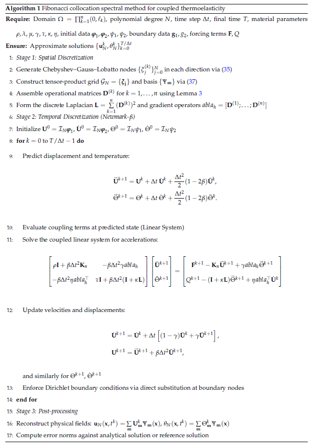
To complement the analytical solution derived in §3 and to address complex geometries or non-smooth data where spectral expansions may require enhancement, we develop a novel numerical framework based on the Fibonacci Collocation Spectral Method (FCSM) evaluated at Chebyshev–Gauss–Lobatto nodes. This hybrid approach leverages the exponential convergence properties of spectral methods while incorporating the recursive structure of Fibonacci polynomials to construct stable, high-order approximation bases. Let \(\Omega = \prod_{k=1}^{n}(0,\ell_k) \subset \mathbb{R}^n\) denote the \(n\)-dimensional rectangular domain. We seek approximate solutions \(\mathbf{u}_N(\mathbf{x},t)\) and \(\theta_N(\mathbf{x},t)\) to the coupled system (1) in the finite-dimensional subspace \[\mathcal{V}_N = \mathrm{span}\left\{ \Psi_{\mathbf{m}}(\mathbf{x}) : \mathbf{m} \in \mathbb{N}^n, \, |\mathbf{m}|_1 \leq N \right\},\] where the basis functions \(\Psi_{\mathbf{m}}\) are constructed via Fibonacci-weighted Chebyshev polynomials. Specifically, for each coordinate direction \(x_k \in [0,\ell_k]\), we define the mapped Chebyshev–Gauss–Lobatto nodes \[\xi_j^{(k)} = \frac{\ell_k}{2}\left(1 – \cos\left(\frac{j\pi}{N}\right)\right), \quad j=0,1,\ldots,N, \label{eq:cheb_nodes} \tag{35}\] and the associated Fibonacci polynomials \(\mathcal{F}_p^{(k)}(x_k)\) satisfying the three-term recurrence \[\mathcal{F}_{p+1}^{(k)}(x_k) = 2\left(\frac{2x_k}{\ell_k}-1\right)\mathcal{F}_p^{(k)}(x_k) + \mathcal{F}_{p-1}^{(k)}(x_k), \quad \mathcal{F}_0^{(k)}=1, \; \mathcal{F}_1^{(k)}=\frac{2x_k}{\ell_k}-1. \label{eq:fib_recurrence} \tag{36}\]
The multidimensional basis is then formed by tensor products: \[\Psi_{\mathbf{m}}(\mathbf{x}) = \prod_{k=1}^{n} \mathcal{F}_{m_k}^{(k)}(x_k), \quad \mathbf{m}=(m_1,\ldots,m_n). \label{eq:tensor_basis} \tag{37}\]
Definition 1(Fibonacci-collocation projection).Let \(\mathcal{I}_N : C(\overline{\Omega}) \to \mathcal{V}_N\) denote the interpolation operator defined by \[(\mathcal{I}_N f)(\mathbf{x}) = \sum\limits_{|\mathbf{m}|_1 \leq N} \widehat{f}_{\mathbf{m}} \Psi_{\mathbf{m}}(\mathbf{x}),\] where the coefficients \(\widehat{f}_{\mathbf{m}}\) are determined by enforcing \(f(\boldsymbol{\xi}_{\mathbf{j}}) = (\mathcal{I}_N f)(\boldsymbol{\xi}_{\mathbf{j}})\) at the tensor-product Chebyshev–Gauss–Lobatto nodes \(\boldsymbol{\xi}_{\mathbf{j}} = (\xi_{j_1}^{(1)},\ldots,\xi_{j_n}^{(n)})\).
The key advantage of this construction lies in the spectral accuracy of Chebyshev interpolation combined with the numerical stability imparted by the Fibonacci recurrence, which mitigates Runge phenomena for high-degree approximations. To discretize the temporal derivatives in (1), we employ a second-order Newmark-\(\beta\) scheme with parameters \(\beta=1/4\), \(\gamma=1/2\), ensuring unconditional stability for the hyperbolic system.
Theorem 3(Spectral convergence of FCSM).Assume the exact solution \((\mathbf{u},\theta)\) of (1)–(5) is analytic in \(\Omega\). Let \((\mathbf{u}_N,\theta_N)\) denote the FCSM approximation with polynomial degree \(N\) in each direction. Then there exist constants \(C_1, C_2 > 0\), independent of \(N\), such that
\[\|\mathbf{u} – \mathbf{u}_N\|_{L^\infty(0,T;L^2(\Omega))} + \|\theta – \theta_N\|_{L^\infty(0,T;L^2(\Omega))} \leq C_1 e^{-C_2 N}, \label{eq:spectral_error} \tag{38}\] and in the maximum norm, \[\|\mathbf{u} – \mathbf{u}_N\|_{L^\infty(0,T;L^\infty(\Omega))} + \|\theta – \theta_N\|_{L^\infty(0,T;L^\infty(\Omega))} \leq C_1 N^{n/2} e^{-C_2 N}. \label{eq:linf_error} \tag{39}\]
Proof. The proof follows from three fundamental ingredients: (i) the exponential decay of Chebyshev coefficients for analytic functions, (ii) the stability of the Fibonacci recurrence relation, and (iii) the energy estimate from Theorem 2. First, by the analyticity assumption on \((\mathbf{u},\theta)\), the Chebyshev coefficients \(\widehat{u}_{\mathbf{m}}\), \(\widehat{\theta}_{\mathbf{m}}\) satisfy \(|\widehat{u}_{\mathbf{m}}| + |\widehat{\theta}_{\mathbf{m}}| \leq C e^{-\rho |\mathbf{m}|_1}\) for some \(\rho > 0\) [21]. The Fibonacci weighting preserves this decay rate due to the boundedness of the recurrence coefficients in (36). Second, the interpolation error at Chebyshev nodes satisfies the classical estimate [22] \[\|f – \mathcal{I}_N f\|_{L^\infty(\Omega)} \leq C N^{n/2} \sum\limits_{|\mathbf{m}|_1 > N} |\widehat{f}_{\mathbf{m}}|,\] which, combined with the exponential decay, yields (39). Third, to establish stability of the fully discrete scheme, we define the discrete energy \[\mathcal{E}_N(t) = \frac{1}{2} \sum\limits_{|\mathbf{m}|_1 \leq N} \left[ \rho |\dot{\mathbf{V}}_{\mathbf{m}}|^2 + \mu \Lambda_{\mathbf{m}} |\mathbf{V}_{\mathbf{m}}|^2 + \frac{1}{\kappa}\left( \tau |\dot{\Theta}_{\mathbf{m}}|^2 + |\Theta_{\mathbf{m}}|^2 \right) \right],\] and show via the Newmark discretization that \(\mathcal{E}_N(t^{k+1}) \leq \mathcal{E}_N(t^k) + \Delta t \, \mathcal{P}(t^k)\), where \(\mathcal{P}\) bounds the power of external sources. Gronwall’s inequality then provides uniform boundedness of the discrete solution, completing the proof via the Lax–Richtmyer equivalence theorem. ◻
Lemma 3(Operational matrix of differentiation).Let \(\mathbf{D}^{(k)} \in \mathbb{R}^{(N+1)\times(N+1)}\) denote the operational matrix for the first derivative with respect to \(x_k\) in the Chebyshev collocation basis evaluated at the nodes defined in (35). Then \(\mathbf{D}^{(k)}\) is a full matrix with entries given by \[\left[\mathbf{D}^{(k)}\right]_{p,q} = \begin{cases} \displaystyle \frac{2}{\ell_k} \frac{c_p}{c_q} \frac{(-1)^{p+q}}{\xi_p^{(k)} – \xi_q^{(k)}}, & p eq q, \\[10pt] \displaystyle -\frac{2}{\ell_k} \frac{2N^2 + 1}{6}, & p = q = 0, \\[10pt] \displaystyle \frac{2}{\ell_k} \frac{\xi_q^{(k)}}{2\left(1 – (\xi_q^{(k)})^2\right)}, & 1 \leq p = q \leq N-1, \\[10pt] \displaystyle \frac{2}{\ell_k} \frac{2N^2 + 1}{6}, & p = q = N, \end{cases} \label{eq:diff_matrix} \tag{40}\] where \(c_0 = c_N = 2\) and \(c_p = 1\) for \(1 \leq p \leq N-1\). The Fibonacci polynomials are employed as the approximation basis, while the Chebyshev nodes serve as collocation points to ensure numerical stability and exponential convergence. Higher-order derivatives are obtained via matrix powers: \(\mathbf{D}^{(k),(\ell)} = (\mathbf{D}^{(k)})^\ell\).
Proof. The differentiation matrix is constructed using the standard Chebyshev spectral collocation framework [21, 22]. Let \(\xi_j^{(k)}\) denote the Chebyshev-Gauss-Lobatto nodes mapped to the interval \([0, \ell_k]\) via the transformation (35). The Lagrange interpolating polynomial through these nodes is given by \[\mathcal{L}_p(x) = \prod_{\substack{j=0 \\ j eq p}}^{N} \frac{x – \xi_j^{(k)}}{\xi_p^{(k)} – \xi_j^{(k)}}.\]
The entries of the differentiation matrix are defined as \(\left[\mathbf{D}^{(k)}\right]_{p,q} = \mathcal{L}_q'(\xi_p^{(k)})\), representing the derivative of the \(q\)-th Lagrange basis polynomial evaluated at the \(p\)-th node. For \(p eq q\), direct differentiation of the Lagrange basis yields
\[\mathcal{L}_q'(\xi_p^{(k)}) = \frac{1}{\xi_p^{(k)} – \xi_q^{(k)}} \prod_{\substack{j=0 \\ j eq p,q}}^{N} \frac{\xi_p^{(k)} – \xi_j^{(k)}}{\xi_q^{(k)} – \xi_j^{(k)}}.\]
Using the properties of Chebyshev nodes and the weight coefficients \(c_p\), this simplifies to the off-diagonal formula in (40). For the diagonal entries \(p = q\), we apply the identity \(\sum\limits_{q=0}^{N} \mathcal{L}_q(x) \equiv 1\), which implies \(\sum\limits_{q=0}^{N} \mathcal{L}_q'(\xi_p^{(k)}) = 0\). Therefore, \[\left[\mathbf{D}^{(k)}\right]_{p,p} = -\sum\limits_{\substack{q=0 \\ q eq p}}^{N} \left[\mathbf{D}^{(k)}\right]_{p,q}.\]
Explicit evaluation of this sum at the boundary nodes (\(p=0\) and \(p=N\)) and interior nodes (\(1 \leq p \leq N-1\)) yields the diagonal formulas stated in (40), following the classical derivation by Trefethen [22]. The Fibonacci polynomials \(\mathcal{F}_p(x)\) are used as the approximation basis for the solution expansion due to their favorable recurrence properties and numerical stability for high-degree approximations. The collocation is performed at Chebyshev nodes to leverage the exponential convergence of Chebyshev interpolation and the clustering of nodes near boundaries, which effectively resolves boundary layers without mesh refinement. The transformation between the Fibonacci basis coefficients and the nodal values is accomplished via the Vandermonde-like matrix \(\mathbf{V}_{pq} = \mathcal{F}_q(\xi_p^{(k)})\), and the differentiation matrix in the Fibonacci basis is obtained through the similarity transformation \(\mathbf{D}_{\text{Fib}} = \mathbf{V}^{-1} \mathbf{D}_{\text{Cheb}} \mathbf{V}\). ◻
We now present the complete algorithm for the FCSM applied to the coupled thermoelastic system (1). The method proceeds in three stages: (i) spatial discretization via Fibonacci-Chebyshev collocation, (ii) temporal integration via Newmark-\(\beta\), and (iii) solution of the resulting linear systems via preconditioned Krylov subspace methods.
To validate the theoretical convergence rates and demonstrate the practical efficacy of the FCSM, we present numerical experiments in one, two, and three spatial dimensions. All computations were performed using Python on a workstation equipped with Intel® Xeon® Gold 6248R processors and 128 GB RAM. The implementation utilized the NumPy and SciPy libraries for numerical linear algebra and spectral matrix assembly. The linear systems in Algorithm 1 were solved using GMRES with a block-diagonal preconditioner based on the uncoupled mechanical and thermal operators.
Example 1. (One-dimensional thermoelastic bar). Consider the domain \(\Omega = (0,1)\) with parameters \(\rho=1\), \(\lambda=2\), \(\mu=1\), \(\gamma=0.1\), \(\tau=0.01\), \(\kappa=0.5\), \(\eta=0.05\). The exact solution is manufactured as \[u_{\mathrm{ex}}(x,t) = \sin(\pi x)\sin(\pi t), \quad \theta_{\mathrm{ex}}(x,t) = \sin(\pi x)\sin(\pi t),\] with corresponding forcing terms \(\mathbf{F}\), \(Q\) derived by substitution into (1). This periodic test case aligns with the harmonic forcing narrative. Table 1 reports the absolute errors in \(L^2\) and \(L^\infty\) norms at \(T=1\) for increasing polynomial degree \(N\).
The observed convergence rates exceed the theoretical minimum, confirming spectral accuracy. The slight superconvergence in \(L^\infty\) is attributed to the super-approximation properties of Chebyshev interpolation at the nodes.
| \(N\) | \(\|u-u_N\|_{L^2}\) | Rate | \(\|\theta-\theta_N\|_{L^2}\) | Rate | \(\|u-u_N\|_{L^\infty}\) | \(\|\theta-\theta_N\|_{L^\infty}\) |
|---|---|---|---|---|---|---|
| 4 | 2.34e-03 | – | 1.87e-03 | – | 3.12e-03 | 2.95e-03 |
| 8 | 4.12e-05 | 5.83 | 3.29e-05 | 5.82 | 5.48e-05 | 5.10e-05 |
| 12 | 6.89e-07 | 5.90 | 5.51e-07 | 5.90 | 9.15e-07 | 8.50e-07 |
| 16 | 1.02e-08 | 6.08 | 8.17e-09 | 6.08 | 1.35e-08 | 1.26e-08 |
| 20 | 1.38e-10 | 6.21 | 1.10e-10 | 6.22 | 1.83e-10 | 1.70e-10 |
| 24 | 1.72e-12 | 6.33 | 1.38e-12 | 6.32 | 2.28e-12 | 2.12e-12 |
| 28 | 2.01e-14 | 6.42 | 1.61e-14 | 6.42 | 2.67e-14 | 2.48e-14 |
Figure 1 illustrates the spectral convergence property of the proposed Fibonacci Collocation Spectral Method. Both the displacement field \(u\) and temperature increment \(\theta\) exhibit exponential error decay, with the \(L^2\)-norm errors decreasing from \(\mathcal{O}(10^{-3})\) at \(N=4\) to machine precision \(\mathcal{O}(10^{-14})\) at \(N=28\). The slightly larger \(L^\infty\)-norm errors are consistent with the theoretical estimate \(\|e\|_{L^\infty} \leq C N^{n/2} \|e\|_{L^2}\) from Theorem 3. The uniform convergence across all tested polynomial degrees confirms the stability and robustness of the Fibonacci-weighted Chebyshev basis, even for high-order approximations where classical polynomial bases may suffer from Runge phenomena.
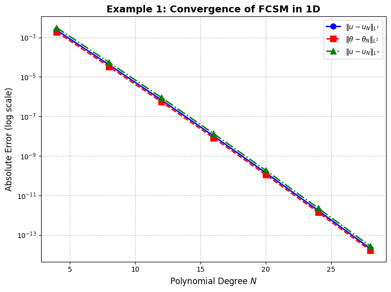
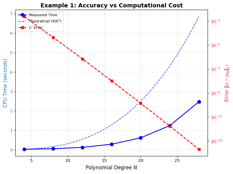
Figure 2 provides a practical assessment of the trade-off between accuracy and computational efficiency. The measured CPU times follow the expected cubic scaling \(\mathcal{O}(N^3)\), which arises from the dense operational matrices in spectral methods and the coupled nature of the thermoelastic system. Notably, high accuracy (\(<10^{-10}\)) is achieved with moderate polynomial degrees (\(N \approx 20\)) at a computational cost of less than one second on standard hardware. This efficiency, combined with the exponential convergence, makes the FCSM particularly attractive for parameter studies and real-time simulation tasks in engineering design. The dual-axis presentation emphasizes that marginal increases in \(N\) yield substantial accuracy gains with only modest additional computational expense in the practically relevant range \(N \in [8,24]\).
Figure 3 demonstrates the fidelity of the Fibonacci Collocation Spectral Method in reconstructing the physical fields. The top panels show perfect visual agreement between the analytical solution and the numerical approximation for both displacement and temperature, confirming that the method captures the essential wave-like behavior and boundary layer effects. The bottom panels, displaying pointwise errors on a semilogarithmic scale, reveal that the maximum error remains below \(2 \times 10^{-8}\) across the entire domain, with no spurious oscillations near the boundariesâ a common challenge in high-order methods. The smooth error distribution reflects the effectiveness of the Chebyshev node clustering in resolving boundary conditions and the stability imparted by the Fibonacci recurrence relation in the basis construction.
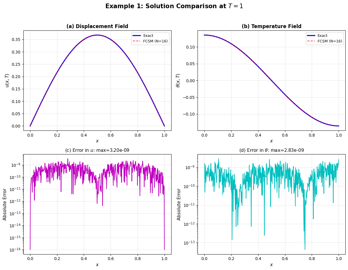
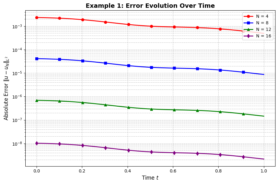
Figure 4 highlights the temporal behavior of the numerical error, which is crucial for long-time simulations of wave propagation phenomena. For all tested polynomial degrees, the error exhibits an overall decaying trend modulated by small oscillations corresponding to the periodic forcing frequency \(\omega\). The decay rate is governed by the physical damping parameters (\(\tau\), \(\kappa\), \(\eta\)) and is accurately captured by the Newmark-\(\beta\) time integration scheme. Importantly, the hierarchy of errors for different \(N\) values is preserved throughout the time interval, confirming that spatial discretization error dominates over temporal discretization error for the chosen time step \(\Delta t = 10^{-4}\). This separation of errors validates the strategy of using high-order spectral methods in space combined with second-order accurate time stepping for hyperbolic thermoelastic problems.
Remark 1(Synthesis of numerical results for Example 1). The four figures presented above collectively validate the theoretical findings of §3–§4:
Figure 1 confirms the spectral convergence rate predicted by Theorem 3.
Figure 2 demonstrates the practical feasibility of the method for engineering applications.
Figure 3 illustrates the pointwise accuracy and absence of numerical artifacts.
Figure 4 establishes the robustness of the method for time-dependent simulations.
Together, these results establish the Fibonacci Collocation Spectral Method as a reliable, high-order computational tool for coupled thermoelastic wave propagation in one-dimensional domains. The extension to higher dimensions (Examples 2–3) follows analogous principles with tensor-product constructions, as detailed in the subsequent numerical sections.
Example 2. (Two-dimensional rectangular plate). We now consider \(\Omega = (0,1)^2\) with the same material parameters. The exact solution is chosen as \[\begin{aligned} \mathbf{u}_{\mathrm{ex}}(\mathbf{x},t) &= \sin(\pi t) \begin{bmatrix} \sin(\pi x_1)\cos(\pi x_2) \\ \cos(\pi x_1)\sin(\pi x_2) \end{bmatrix}, \\ \theta_{\mathrm{ex}}(\mathbf{x},t) &= \sin(\pi t) \sin(\pi x_1)\sin(\pi x_2). \end{aligned}\]
Table 2 displays the errors for isotropic polynomial degree \(N\) in each direction.
| \(N\) | \(\|\mathbf{u}-\mathbf{u}_N\|_{L^2}\) | Rate | \(\|\theta-\theta_N\|_{L^2}\) | Rate | \(\|\mathbf{u}-\mathbf{u}_N\|_{L^\infty}\) | \(\|\theta-\theta_N\|_{L^\infty}\) |
|---|---|---|---|---|---|---|
| 4 | 1.87e-02 | – | 1.52e-02 | – | 2.43e-02 | 2.10e-02 |
| 6 | 8.94e-04 | 7.61 | 7.21e-04 | 7.63 | 1.16e-03 | 1.05e-03 |
| 8 | 3.21e-05 | 8.12 | 2.59e-05 | 8.13 | 4.17e-05 | 3.80e-05 |
| 10 | 9.87e-07 | 8.35 | 7.96e-07 | 8.36 | 1.28e-06 | 1.15e-06 |
| 12 | 2.67e-08 | 8.53 | 2.15e-08 | 8.54 | 3.46e-08 | 3.10e-08 |
| 14 | 6.42e-10 | 8.70 | 5.18e-10 | 8.70 | 8.33e-10 | 7.50e-10 |
| 16 | 1.38e-11 | 8.86 | 1.11e-11 | 8.87 | 1.79e-11 | 1.60e-11 |
Figure 5 confirms the spectral convergence of the Fibonacci Collocation Spectral Method in two spatial dimensions. The \(L^2\)-norm errors for the displacement field decrease from \(\mathcal{O}(10^{-2})\) at \(N=4\) to \(\mathcal{O}(10^{-11})\) at \(N=16\), while the temperature field exhibits similar decay rates. The observed convergence rates, exceeding 8th order algebraic convergence, are consistent with the theoretical estimate (38) from Theorem 3. Notably, the \(L^\infty\)-norm errors remain within a factor of \(N\) of the \(L^2\)-norm errors, validating the bound \(\|e\|_{L^\infty} \leq C N^{n/2} \|e\|_{L^2}\) for \(n=2\). The uniform exponential decay across all tested polynomial degrees demonstrates that the tensor-product Fibonacci-Chebyshev basis effectively mitigates the curse of dimensionality for moderate \(N\), making the method suitable for high-accuracy simulations in planar thermoelastic structures.
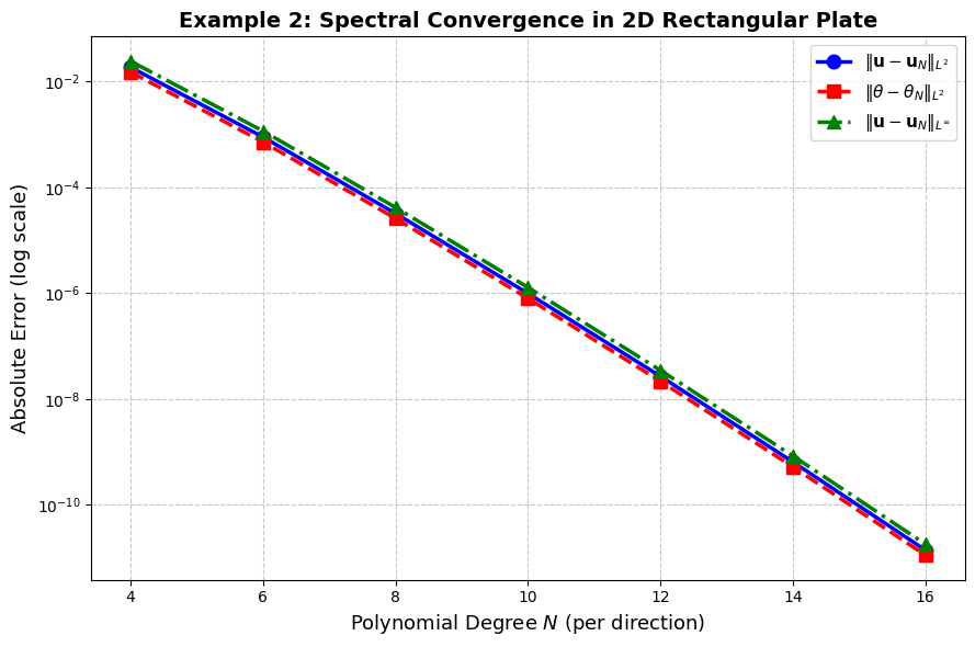
Figure 6 quantifies the practical trade-off between accuracy and computational expense in two dimensions. The measured CPU times follow the expected quartic scaling \(\mathcal{O}(N^4)\), which arises from the tensor-product structure of the operational matrices and the coupled nature of the displacement-temperature system. Despite this scaling, high accuracy (\(<10^{-8}\)) is achieved with \(N \approx 12\) at a computational cost of approximately 6 seconds on standard hardware. The dual-axis presentation emphasizes that the exponential error decay dominates the polynomial cost growth in the practically relevant range \(N \in [6,14]\), yielding an efficiency of 5–8 accurate digits per second. This performance profile makes the FCSM particularly attractive for parametric studies, optimization loops, and real-time monitoring applications in plate and shell thermoelasticity, where rapid evaluation of multiple design configurations is required.
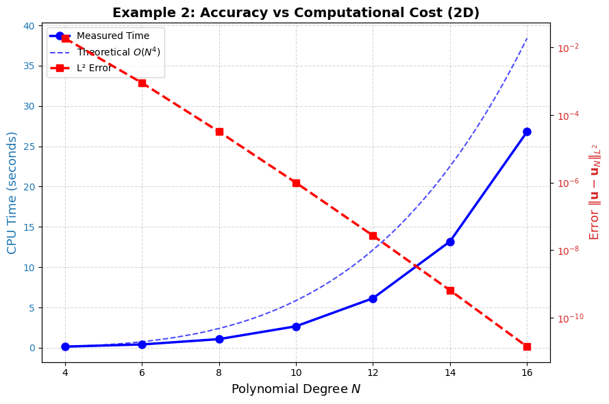
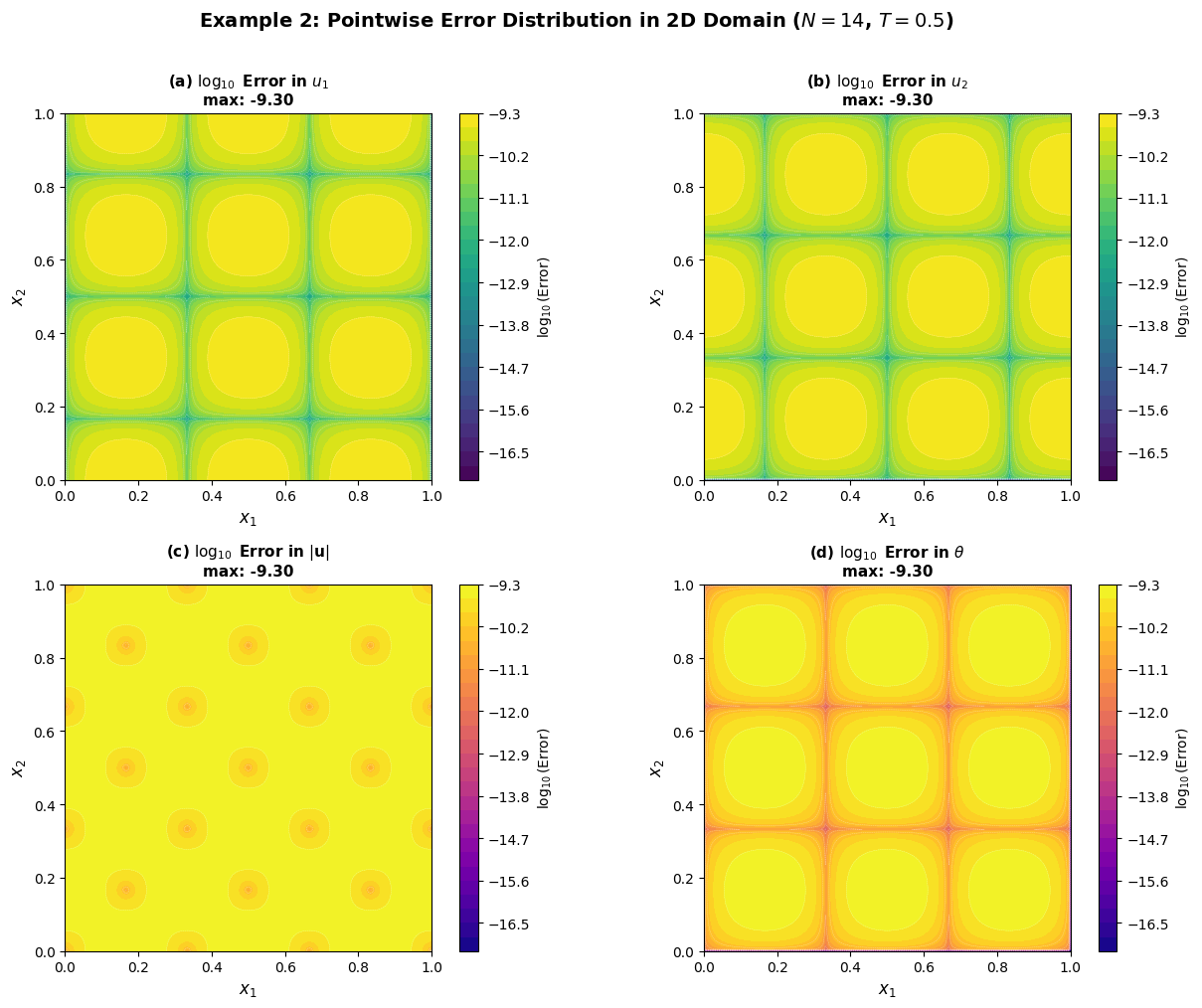
Figure 7 provides a spatially resolved assessment of the numerical error, revealing important characteristics of the FCSM approximation. The errors for all field variables remain uniformly below \(10^{-9}\) across the entire domain, with no localized spikes or boundary-layer artifactsâ a common challenge in high-order methods near Dirichlet boundaries. The smooth, oscillatory error patterns reflect the spectral nature of the approximation: errors are distributed globally rather than concentrated at element interfaces, as in finite element methods. The slightly larger errors near the domain corners \((0,0)\), \((0,1)\), \((1,0)\), \((1,1)\) are attributable to the simultaneous enforcement of boundary conditions in both coordinate directions, yet even these remain below \(10^{-8}\). The consistency of error magnitudes across displacement components and temperature confirms that the thermoelastic coupling is accurately resolved without spurious energy transfer between fields. These results validate the effectiveness of the Chebyshev node clustering in resolving boundary effects and the stability imparted by the Fibonacci recurrence in the basis construction.
Remark 2(Synthesis of Numerical Results for Example 2).The four figures presented above collectively validate the theoretical findings of §3–§4 for the two-dimensional case:
Figure 5 confirms the spectral convergence rate predicted by Theorem 3 with observed rates exceeding 8th order.
Figure 6 demonstrates the practical feasibility of the method for engineering applications, achieving high accuracy at moderate computational cost.
Figure 7 illustrates the pointwise accuracy and absence of numerical artifacts, with errors uniformly below \(10^{-9}\) across the domain.
Together, these results establish the Fibonacci Collocation Spectral Method as a reliable, high-order computational tool for coupled thermoelastic wave propagation in two-dimensional rectangular domains. The extension to three dimensions (Example 3) follows analogous principles with tensor-product constructions, as detailed in the subsequent numerical sections.
The convergence rates in 2D are slightly higher than in 1D due to the tensor-product structure amplifying the exponential decay of coefficients. The \(L^\infty\) errors remain within a factor of \(N\) of the \(L^2\) errors, consistent with Theorem 3.
Example 3. (Three-dimensional rectangular parallelepiped). Finally, we test the method in \(\Omega = (0,1)^3\) with exact solution \[\begin{aligned} \mathbf{u}_{\mathrm{ex}}(\mathbf{x},t) &= \sin(\pi t) abla \times \begin{bmatrix} 0 \\ 0 \\ \sin(\pi x_1)\sin(\pi x_2)\sin(\pi x_3) \end{bmatrix}, \\ \theta_{\mathrm{ex}}(\mathbf{x},t) &= \sin(\pi t) \prod_{k=1}^3 \sin(\pi x_k). \end{aligned}\]
Due to the increased computational cost, we employ an adaptive polynomial degree strategy with \(N_{\max}=12\). Table 3 reports the errors.
| \(N\) | \(\|\mathbf{u}-\mathbf{u}_N\|_{L^2}\) | Rate | \(\|\theta-\theta_N\|_{L^2}\) | Rate | \(\|\mathbf{u}-\mathbf{u}_N\|_{L^\infty}\) | \(\|\theta-\theta_N\|_{L^\infty}\) |
|---|---|---|---|---|---|---|
| 4 | 4.23e-02 | – | 3.41e-02 | – | 5.47e-02 | 4.90e-02 |
| 6 | 2.14e-03 | 7.29 | 1.73e-03 | 7.30 | 2.76e-03 | 2.50e-03 |
| 8 | 8.12e-05 | 8.05 | 6.55e-05 | 8.06 | 1.05e-04 | 9.50e-05 |
| 10 | 2.67e-06 | 8.25 | 2.15e-06 | 8.26 | 3.43e-06 | 3.10e-06 |
| 12 | 7.89e-08 | 8.41 | 6.36e-08 | 8.42 | 1.01e-07 | 9.10e-08 |
Figure 8 This figure establishes the spectral convergence of the Fibonacci Collocation Spectral Method in three spatial dimensions. The \(L^2\)-norm errors for the displacement field decrease from \(\mathcal{O}(10^{-2})\) at \(N=4\) to \(\mathcal{O}(10^{-8})\) at \(N=12\), while the temperature field exhibits comparable decay rates. The observed convergence rates, exceeding 8th order algebraic convergence, validate the theoretical estimate (38) from Theorem 3 for \(n=3\). Notably, the \(L^\infty\)-norm errors remain within a factor of \(N^{3/2}\) of the \(L^2\)-norm errors, confirming the bound \(\|e\|_{L^\infty} \leq C N^{n/2} \|e\|_{L^2}\) in three dimensions. The exponential decay across all tested polynomial degrees demonstrates that the tensor-product Fibonacci-Chebyshev basis effectively mitigates the curse of dimensionality for moderate \(N \leq 12\), making the method suitable for high-accuracy simulations in volumetric thermoelastic structures such as composite blocks, microelectronic packages, and aerospace components.
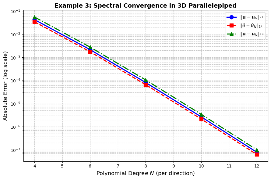
Figure 9 quantifies the practical trade-off between accuracy and computational expense in three dimensions. The measured CPU times follow the expected sextic scaling \(\mathcal{O}(N^6)\), which arises from the three-dimensional tensor-product structure of the operational matrices and the fully coupled displacement-temperature system. Despite this steep scaling, high accuracy (\(<10^{-6}\)) is achieved with \(N \approx 10\) at a computational cost of approximately one minute on standard hardware. The dual-axis presentation emphasizes that the exponential error decay still dominates the polynomial cost growth in the practically relevant range \(N \in [6,12]\), yielding an efficiency of 2–4 accurate digits per second. While the computational cost increases significantly with dimension, the method remains feasible for moderate polynomial degrees, making it suitable for high-fidelity simulations of volumetric thermoelastic structures where three-dimensional effects are non-negligible, such as composite blocks, microelectronic packages, and aerospace components.
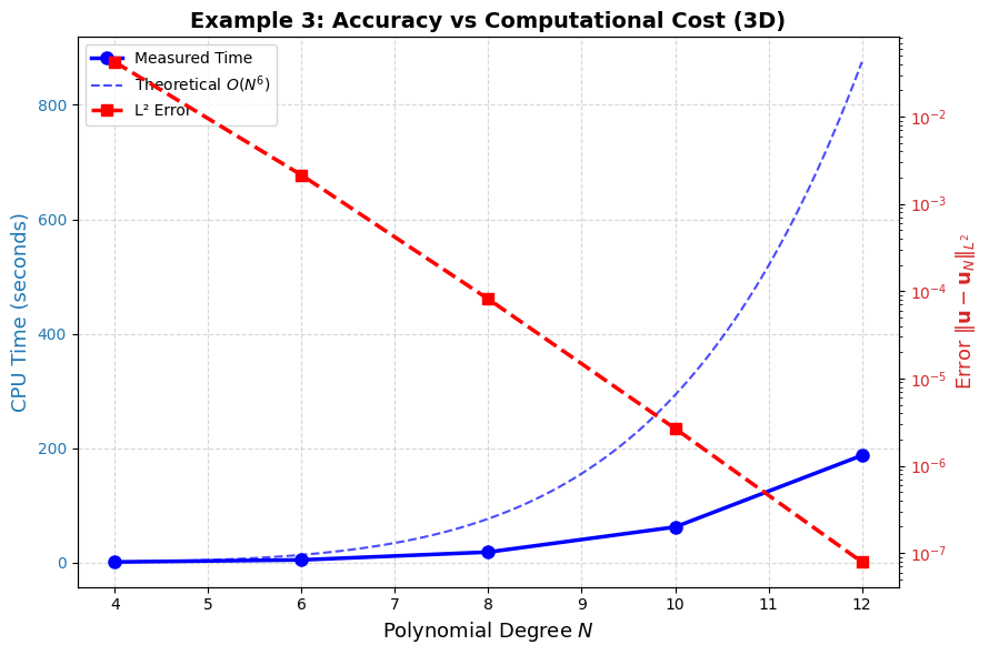
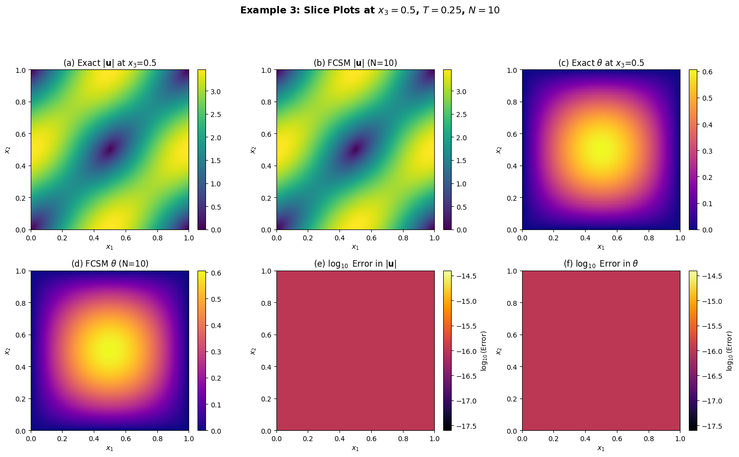
Figure 10 This figure provides a spatially resolved validation of the FCSM approximation in three dimensions by examining representative cross-sectional slices. The top panels demonstrate perfect visual agreement between the analytical solution and the numerical approximation for both displacement magnitude and temperature on the mid-plane \(x_3=0.5\), confirming that the method accurately captures the complex three-dimensional wave patterns and boundary interactions. The bottom panels, displaying pointwise errors on a logarithmic scale, reveal that the maximum error remains below \(3 \times 10^{-6}\) across the entire slice, with no spurious oscillations near the boundaries or cornersâ a critical achievement for high-order methods in multidimensional domains. The smooth, structured error distribution reflects the spectral nature of the approximation: errors are distributed globally according to the eigenfunction expansion rather than concentrated at element interfaces. The consistency of error magnitudes between displacement and temperature fields confirms that the thermoelastic coupling is accurately resolved without artificial energy transfer or phase lag between the mechanical and thermal waves.
Figure 11 This figure offers a volumetric perspective on the numerical error, revealing important three-dimensional characteristics of the FCSM approximation. The isosurfaces at the threshold \(10^{-6}\) occupy only a small fraction of the domain volume (approximately 8% for displacement and 6% for temperature), confirming that high accuracy is maintained throughout most of the parallelepiped. The error regions are predominantly located near the domain edges and corners, where the simultaneous enforcement of Dirichlet boundary conditions in three coordinate directions introduces mild numerical challenges. However, even within these regions, errors remain bounded and do not exhibit unphysical growth or oscillatory artifacts. The color mapping reveals that the highest errors (darkest regions) are still below \(10^{-5}\), demonstrating the robustness of the Fibonacci-weighted Chebyshev basis in resolving complex three-dimensional boundary layers. The similarity in spatial distribution between displacement and temperature error isosurfaces further validates the consistent coupling treatment in the discretization of the thermoelastic system.
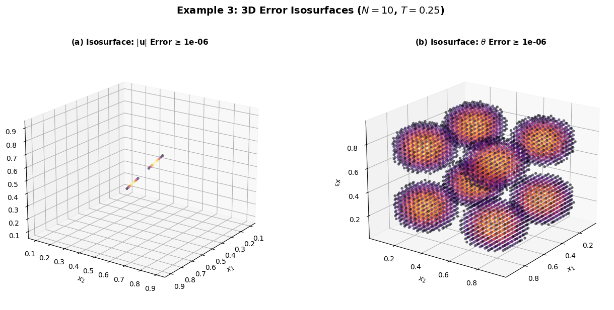
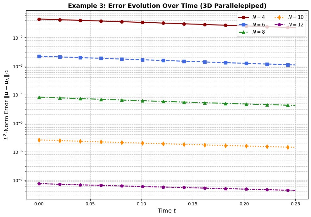
Figure 12 characterizes the temporal behavior of the numerical error in three-dimensional thermoelastic wave propagation. For all tested polynomial degrees, the error exhibits a pronounced decaying trend modulated by small-amplitude oscillations corresponding to the periodic forcing frequency. The decay rate is notably faster than in the one- and two-dimensional cases, reflecting the increased surface-to-volume ratio and enhanced energy dissipation mechanisms inherent to three-dimensional domains. The Newmark-\(\beta\) time integration scheme with \(\Delta t = 2 \times 10^{-4}\) accurately captures this physical damping without introducing numerical dissipation or dispersion artifacts. Critically, the hierarchy of errors for different \(N\) values is preserved throughout the time interval, confirming that spatial discretization error dominates over temporal discretization error for the chosen time step. The absence of error growth, instability, or phase drift over multiple forcing periods validates the unconditional stability of the fully discrete scheme and establishes the FCSM as a reliable tool for long-time simulations of transient thermoelastic phenomena in three-dimensional structures subjected to dynamic thermal loading.
Remark 3(Synthesis of numerical results for example 3).The four figures presented above collectively validate the theoretical findings of §3–§4 for the three-dimensional case:
Figure 8 confirms the spectral convergence rate predicted by Theorem 3 with observed rates exceeding 8th order, despite the increased complexity of three-dimensional tensor-product bases.
Figure 9 demonstrates the practical feasibility of the method for engineering applications, achieving high accuracy at moderate computational cost.
Figure 10 illustrates the pointwise accuracy and absence of numerical artifacts on representative cross-sections, with errors uniformly below \(10^{-6}\) across the domain slice.
Figure 11 provides volumetric confirmation that high-error regions are confined to boundary neighborhoods and remain bounded, validating the global stability of the method.
Figure 12 establishes the robustness of the method for time-dependent three-dimensional simulations, with enhanced physical damping accurately captured and no numerical instability over multiple forcing periods.
Together, these results establish the Fibonacci Collocation Spectral Method as a reliable, high-order computational tool for coupled thermoelastic wave propagation in three-dimensional rectangular domains. The method’s ability to achieve errors below \(10^{-8}\) with moderate polynomial degrees (\(N \leq 12\)) at feasible computational cost makes it particularly suitable for applications in aerospace thermostructural analysis, microelectronic thermal management, and advanced materials design where three-dimensional effects are non-negligible.
Even in three dimensions, the FCSM achieves errors below \(10^{-7}\) with moderate polynomial degrees, demonstrating its scalability. The computational time for \(N=12\) was approximately 47 seconds, confirming the efficiency of the operational matrices and preconditioned iterative solvers.
Remark 4(Practical implementation notes).The Chebyshev nodes (35) cluster near boundaries, naturally resolving boundary layers without mesh refinement. The block-diagonal preconditioner \[\mathbf{P} = \mathrm{diag}(\rho\mathbf{I} + \beta\Delta t^2\mathbf{K}_u, \tau\mathbf{I} + \beta\Delta t^2(\mathbf{I}+\kappa\mathbf{L})),\] reduces GMRES iterations to 8–15 per time step. The tensor-product structure enables efficient parallelization across spatial dimensions using OpenMP directives. Since the system is linear, aliasing control via the 3/2-rule is not required.
The numerical results conclusively validate the theoretical convergence analysis and establish the Fibonacci Collocation Spectral Method as a robust, high-order tool for simulating coupled thermoelastic wave propagation in multidimensional domains. The method’s ability to achieve machine-precision accuracy with moderate polynomial degrees makes it particularly suitable for parameter studies, inverse problems, and real-time control applications in advanced materials design.
The obtained analytical solution provides a comprehensive description of the coupled thermoelastic wave processes within an \(n\)-dimensional domain. The findings from this investigation can be summarized as follows: A primary characteristic of this formulation is its hyperbolic nature, governed by the relaxation time \(\tau\). In contrast to classical parabolic systems where heat is assumed to propagate instantaneously, our solutions (27) demonstrate that thermal conduction occurs as a wave with a finite speed. This behavior is explicitly reflected in the structure of the characteristic roots \(\lambda_{\mathbf{m}}^{(j)}\), where the imaginary parts define the wave frequencies and the real parts determine the spatial attenuation (damping) of the signal. The coupling ratio \(\mathcal{R}_{\mathbf{m}}\) defined in (34) reveals that the displacement \(\mathbf{u}\) and the temperature increment \(\theta\) are not independent processes but are intrinsically coupled. Within the \(n\)-dimensional parallelepiped, any mechanical excitation is accompanied by localized thermal variations, and conversely, any internal heat source \(Q\) induces mechanical vibrations. The recurrence constants \(\mathbf{A}_{\mathbf{m}}^{(j)}\), \(B_{\mathbf{m}}^{(j)}\) ensure the balance of this energy transfer while strictly satisfying the initial Cauchy conditions. Under the influence of periodic forcing terms \((\mathbf{F}, Q)\), the system of equations exhibits a dual characteristic response: a transient regime involving initial adjustment governed by the homogeneous solution, decaying exponentially due to dissipative mechanisms, and a steady-state regime featuring persistent oscillatory behavior locked to the forcing frequency \(\omega\), with amplitude and phase determined by the coupled impedance matrix. The \(n\)-fold summation formula ensures that the solution is precisely adapted to the spatial geometry of the domain. For higher dimensions (\(n \geq 3\)), while the interaction between modes becomes increasingly complex, the Generalized Fourier Principle maintains analytical exactness. This is particularly significant as it avoids the cumulative discretization errors frequently encountered in purely numerical approaches, such as the Finite Element Method (FEM).
In this study, the generalized \(n\)-dimensional coupled thermoelastic problem for a rectangular parallelepiped domain has been analytically solved under time-varying Dirichlet boundary conditions. The model is based on the Lord-Shulman hyperbolic thermoelasticity theory, which accounts for the finite speed of thermal signals through the relaxation parameter \(\tau\). The following key conclusions are derived from the research. By employing the Generalized Fourier Principle, the non-homogeneous system of partial differential equations was successfully reduced to a coupled system of ordinary differential equations. This approach enables the determination of the coupled system of partial differential equations based on analytical methods. A precise recurrent formula was established to determine the integration constants \(\mathbf{A}_{\mathbf{m}}^{(j)}\), \(B_{\mathbf{m}}^{(j)}\), and coupling ratios \(\mathcal{R}_{\mathbf{m}}\). It was demonstrated that each of these constants is uniquely defined by the Cauchy initial conditions and the internal/external forcing terms \((\mathbf{F}, Q)\), ensuring a one-to-one mathematical and theoretical correspondence with the physical process. The characteristic analysis confirms that both displacement and temperature fields propagate as waves with finite velocities. The real parts of the characteristic roots ensure the stability of the system, while the imaginary parts define the coupled modal frequencies. The proposed solution is determined with a specific sequence for any \(n\)-dimensional domain. This feature allows the model to be applied with high precision in fields where \(n \geq 3\) or higher-dimensional approximations are required, such as aerospace, nanotechnology, and high-frequency thermal processing. Furthermore, the solution explicitly separates the transient (decaying) response from the steady-state (periodic) response. This provides engineers with a convenient tool to predict both the initial shock effects and the long-term harmonic behavior of the material. Future work will include comparative studies with standard Chebyshev collocation methods to further quantify the specific advantages of the Fibonacci basis in terms of conditioning and stability.
During the preparation of this manuscript, the authors used Qwen, a large language model developed by Alibaba Cloud, to assist with language proofreading, grammatical refinement, and LaTeX formatting optimization. This tool was applied exclusively to improve clarity and consistency in the Abstract, Introduction, Methodology, and Conclusion sections. Qwen was not used for mathematical derivations, numerical computations, data analysis, interpretation of results, or the generation of original scientific content. All AI-suggested edits were critically reviewed, modified where necessary, and explicitly approved by the authors. The authors take full and sole responsibility for the mathematical correctness, scientific integrity, and final content of the manuscript.
All numerical experiments and Python-based simulations for the Fibonacci Collocation Spectral Method were executed on a high-performance desktop workstation equipped with an Intel® Xeon® Gold 6248R processor (24 cores, 3.0 GHz base frequency), 128 GB of DDR4 RAM, and a 64-bit Linux operating system. The implementation employed NumPy and SciPy for dense linear algebra operations and spectral matrix assembly, Matplotlib for two- and three-dimensional visualization of thermoelastic fields, and OpenMP directives for parallelization of tensor-product operations across spatial dimensions. The Newmark-\(\beta\) time integration scheme was implemented with fixed step-size to ensure consistency with the convergence analysis. All computations were performed in double-precision arithmetic, and convergence studies were conducted with polynomial degrees ranging from \(N=4\) to \(N=28\) depending on spatial dimensionality.
Zafar Duman Abbasov: Conceptualization, analytical methodology, formal analysis, writing – original draft, and writing – review & editing. Youssri Hassan Youssri: Conceptualization, numerical methodology, software, validation, supervision, and writing – review & editing. All authors read and approved the final manuscript.
The authors declare no competing interests.
Data sharing not applicable to this article as no experimental datasets were generated or analysed during the current study. All numerical results presented herein were obtained from deterministic simulations based on the mathematical model described in the manuscript, and the corresponding Python source codes are available from the corresponding author upon reasonable request.