
This article develops duality principles applicable to a large class of models in the calculus of variations. We present applications to the full Ginzburg-Landau in superconductivity in the presence of a magnetic field and respective magnetic potential.
We emphasize the results on duality theory here addressed and developed are inspired mainly in the approaches of J.J. Telega, W.R. Bielski and co-workers presented in the articles [1–4]. Other main reference is the article by Toland, [5].
Moreover, details on the Sobolev spaces involved may be found in [6] and basic theoretical results in superconductivity may be found in [7,8].
Similar results and models are addressed in [9–16].
Basic results on convex analysis are addressed in [17,18]. Finally, other related results may be found in [19,20].
Now we start to describe the primal variational formulation for the Ginzburg-Landau model in superconductivity in question.
Let \(\Omega, \Omega_1 \subset \mathbb{R}^3\) be open, bounded and connected sets such that \(\overline{\Omega} \subset \Omega_1\) and \(\Omega_1\) is convex.
Denote the boundaries of \(\Omega\) and \(\Omega_1\) by \(\partial \Omega\) and \(\partial \Omega_1\), respectively.
Denote also by \(|\phi|^2\) the density of super-conducting electrons in the superconductor sample \(\Omega\) and by \(\mathbf{A}\) the magnetic potential on the set \(\Omega_1\). Moreover, define the Ginzburg-Landau functional \(J:V=V_1 \times V_2 \rightarrow \mathbb{R}\), by \[ J(\phi, \mathbf{A})= \frac{\gamma}{2}\int_\Omega |\nabla \phi-i \;\rho \mathbf{A}\phi|^2\;dx +\frac{\alpha}{2}\int_\Omega (|\phi|^2-\beta)^2\;dx+\frac{1}{8\pi}\|\text{ Curl } \mathbf{A}-\mathbf{B}_0\|_{0,2,\Omega_1}^2.\tag{1} \]
Here, \[V_1=W^{1,2}(\Omega; \mathbb{C}),\] and we also set \[V_2= W^{1,2}(\Omega_1; \mathbb{R}^3),\] where \(\gamma>0\), \(\alpha>0\), \(\beta>0\), \(\rho>0\), \(i\) denotes complex imaginary unit and \(\mathbf{B}_0 \in W^{1,2}(\Omega_1; \mathbb{R}^3)\cap C(\overline{\Omega_1};\mathbb{R}^3)\) denotes an external magnetic field.
In the first part of this article, we obtain a global minimizer \((\phi_0,\mathbf{A}_0) \in V\) for \(J\).
We assume also the restriction concerning the London Gauge, that is,
\[\text{ div } \mathbf{A}=0, \text{ in } \Omega_1,\] and \[\mathbf{A} \cdot \mathbf{n}=0, \text{ on } \partial \Omega_1.\]
From the variation of \(J\) in \(\phi\), we obtain
\[ -\text{ div }(\gamma (\nabla \phi-i \rho \mathbf{A}\phi))+\gamma (\nabla \phi-i \rho \mathbf{A}\phi)(-i\rho\mathbf{A})+2\alpha(|\phi|^2-\beta)\phi = 0, \text{ in } \Omega,\tag{2} \]
\[\gamma (\nabla \phi-i\rho\mathbf{A}\phi) \cdot \mathbf{n}=0, \text{ on } \partial \Omega.\]
From the variation of \(J\) in \(\mathbf{A}\), we obtain
\[ \text{ Curl} \left(\text{ Curl } \mathbf{A}-\mathbf{B}_0\right)+\text{ Re }(\gamma (\nabla \phi-i \rho\mathbf{A}\phi)(-i \rho\phi)) =\mathbf{0}, \text{ in } \Omega.\tag{3} \] and \[\text{ Curl } (\text{ Curl } \mathbf{A}) -\text{ Curl } \mathbf{B}_0=\mathbf{0}, \text{ in } \Omega_1\setminus \Omega.\]
Finally, from the London Gauge (we explain in the next section why is not necessary a Lagrange multiplier for such a restriction), we have
\[\text{ div } \mathbf{A}=0, \text{ in } \Omega_1,\] and \[\mathbf{A} \cdot \mathbf{n}=0, \text{ on } \partial \Omega_1.\]
In this section we develop a proof of existence of solution for such a Ginzburg-Landau system in the presence of a magnetic field and concerning potential, as it has been described in the previous section. We emphasize similar models are addressed in [7,8].
We also highlight similar existence results have been presented in the books [9] and [13].
Even though originally a similar existence result have been presented in the book [9], such a result has not been so far peer reviewed by a Journal.
This is the reason we present here such an existence result in details.
Finally, as a previous related existence result we would cite [10].
Theorem 1. Consider again the functional \(J: V \rightarrow \mathbb{R}\) where \[ J(\phi,\mathbf{A})= \frac{\gamma}{2}\int_\Omega |\nabla \phi-i \rho\mathbf{A}\phi|^2\;dx +\frac{\alpha}{2}\int_\Omega (|\phi|^2-\beta)^2\;dx + \frac{1}{8\pi}\int_{\Omega_1} | \text{ Curl } \mathbf{A}-\mathbf{B}_0|^2\;dx.\tag{4} \]
Under these hypotheses and those stated in the previous section, there exists \((\phi_0,\mathbf{A}_0) \in V\) such that \[J(\phi_0,\mathbf{A}_0) =\min_{(\phi,\mathbf{A}) \in V}\{J(\phi,\mathbf{A})\}.\]
Proof. Define \[\alpha_3=\inf_{(\phi,\mathbf{A}) \in V}\{J(\phi,\mathbf{A})\} \in \mathbb{R}.\]
Let \((\phi_n, \mathbf{A}_n) \subset V\) be a sequence such that \[\lim_{n \rightarrow \infty} J(\phi_n,\mathbf{A}_n)=\alpha_3.\]
From the expression of \(J\), there exists \(K_1>0\) such that \[\|\text{Curl} (\mathbf{A}_n)\|_2^2 \leq K_1, \; \forall n \in \mathbb{N}.\]
Given \((\phi,\mathbf{A}) \in V,\) define \((\phi’, \mathbf{A}’) \in V\) by \[\phi’=\phi e^{i\rho \varphi},\] and \[\mathbf{A}’=\mathbf{A}+\nabla \varphi,\] where \(\varphi\) will be specified in the next lines.
Observe that,
\[\begin{aligned} |\nabla \phi’-i \rho \mathbf{A}’ \phi’|_2 =& |\nabla(\phi e^{i\rho \varphi})-i\rho(\mathbf{A}+\nabla \varphi)\phi e^{i\rho \varphi}|_2 \nonumber \\ =& |\nabla \phi (e^{i\rho \varphi})+\phi i\rho e^{i\rho \varphi}\nabla \varphi -i \rho\mathbf{A}\phi e^{i\rho \varphi}-i\rho\phi\nabla \varphi e^{i \rho \varphi}|_2 \nonumber \\ =& |(\nabla \phi-i \rho \mathbf{A}\phi)e^{i\rho \varphi}|_2 \nonumber \\ =& |\nabla \phi-i \rho \mathbf{A}\phi|_2. \end{aligned}\tag{5}\]
Moreover \[\text{Curl}(\mathbf{A}’)=\text{Curl}(\mathbf{A})+\text{Curl}(\nabla \varphi)=\text{Curl}(\mathbf{A}).\]
Also \[|\phi’|=|\phi e^{i \rho \varphi}|=|\phi|.\]
From these last calculations, we may infer the system gauge invariance, that is, \[J(\phi,\mathbf{A})=J(\mathbf{\phi’},\mathbf{A}’).\]
In particular, we shall choose \(\varphi \in W^{1,2}(\Omega_1)\) such that \[div(\mathbf{A}’)=div(\mathbf{A})+\nabla^2\varphi=0,\] and, denoting by \(\mathbf{n}\) the outward normal to \(\partial \Omega_1\), \[\mathbf{A}’\cdot \mathbf{n}=\mathbf{A}\cdot\mathbf{n}+\nabla \varphi \cdot \mathbf{n}=0, \text{ on } \partial \Omega_1,\] that is, \[\nabla^2 \varphi=-div(\mathbf{A}),\; \text{ in } \Omega_1,\] \[\nabla \varphi \cdot \mathbf{n}=-\mathbf{A}\cdot \mathbf{n},\; \text{ on } \partial \Omega_1.\]
Observe that at first we would have, \[\inf_{(\phi,\mathbf{A}) \in V} J(\phi,\mathbf{A}) \leq \inf_{(\phi’,\mathbf{A}’) \in V} J(\phi’,\mathbf{A}’).\]
However \[J(\phi’_n,\mathbf{A}’_n)=J(\phi_n,\mathbf{A}_n) \rightarrow \alpha_3, \; \text{ as } n \rightarrow \infty,\] so that \[\inf_{(\phi,\mathbf{A}) \in V} J(\phi,\mathbf{A}) = \inf_{(\phi’,\mathbf{A}’) \in V} J(\phi’,\mathbf{A}’).\]
From Friedrichs’ inequality, we have, \[\begin{aligned} K_1^2 \geq& \|\text{Curl} (\mathbf{A}_n)\|_2^2 \nonumber \\ =& \|\text{ Curl}(\mathbf{A}’_n)\|_2^2+\|\text{ div }(\mathbf{A}’_n)\|_2^2 \geq K_2\|\mathbf{A}’_n\|_{1,2}^2, \; \forall n \in \mathbb{N}, \end{aligned}\tag{6}\] for some \(K_2>0\).
Hence, \[\|\mathbf{A}’_n\|_{1,2} \leq K_3, \forall n \in \mathbb{N},\] for some \(K_3>0.\)
From such a result and the Sobolev Imbedding theorem, there exists \(K_8>0\) such that
\[\|\mathbf{A}’_n\|_{0,4} \leq K_8, \forall n \in \mathbb{N},\] and \[\|\mathbf{A}’_n\|_{0,2} \leq K_8, \forall n \in \mathbb{N}.\]
Also, from the expression of \(J\), clearly there exists a real constant \(K_9>0\) such that \[\|(\phi)_n’\|_{0,4} = \|(\phi)_n\|_{0,4} \leq K_9, \forall n \in \mathbb{N},\] and since \(\Omega\) is bounded, such a \(K_9>0\) may be also such that \[\|(\phi)_n’\|_{0,2} = \|(\phi)_n\|_{0,2} \leq K_9, \forall n \in \mathbb{N}.\]
Hence, \[\begin{aligned} J(\phi’_n,\mathbf{A}’_n)=& \frac{\gamma}{2}\int_\Omega|\nabla (\phi)’_n-i \rho \mathbf{A}’_n(\phi)’_n|^2_2\;dx +\frac{\alpha}{2}\int_\Omega (|(\phi)’_n|^2-\beta)^2\;dx + \frac{1}{8\pi}\int_{\Omega_1} |\text{Curl}(\mathbf{A}’_n)-\mathbf{B}_0|_2^2\;dx \nonumber \\ \geq& \frac{\gamma}{2}\int_\Omega|\nabla (\phi)’_n|^2\;dx-\gamma |\rho|\|(\phi)_n’\|_{0,4}\|\mathbf{A}_n’\|_{0,4}\|\nabla (\phi)_n’\|_{0,2} +\frac{\gamma}{2}|\rho|^2\|\mathbf{A}_n’ (\phi)’_n\|_{0,2}^2 \nonumber \\ &+\frac{\alpha}{2}\int_\Omega (|(\phi)’_n|^2-\beta)^2\;dx + \frac{1}{8\pi}\int_{\Omega_1} |\text{Curl}(\mathbf{A}’_n)-\mathbf{B}_0|_2^2\;dx \nonumber \\ \geq& \frac{\gamma}{2}\|\nabla (\phi)’_n\|^2_2\;dx-\gamma K_8 K_9 |\rho|\|\nabla (\phi)_n’\|_2 +\frac{\gamma}{2}|\rho|^2\|\mathbf{A}_n'(\phi)’_n\|_2^2 +\frac{\alpha}{2}\int_\Omega (|(\phi)’_n|^2-\beta)^2\;dx \nonumber \\ &+ \frac{1}{8\pi}\int_{\Omega_1} |\text{ Curl}(\mathbf{A}’_n)-\mathbf{B}_0|_2^2\;dx. \end{aligned}\tag{7}\]
Suppose, to obtain contradiction, there exists a subsequence \(\{n_k\}\) such that \[\|\nabla (\phi)’_{n_k}\|_2 \rightarrow +\infty, \text{ as } k \rightarrow \infty.\]
From this and (7) we obtain, \[J(\phi_{n_k}’,\mathbf{A}_{n_k}’) \rightarrow +\infty, \text{ as } k \rightarrow +\infty,\] which contradicts \[J(\phi’_n,\mathbf{A}_n’) \rightarrow \alpha_3, \; \text{ as } n \rightarrow +\infty.\]
Therefore, there exists \(K_4>0\) such that \[\|\nabla (\phi)’_n\|_2 \leq K_4 \in \mathbb{R}^+, \; \forall n \in \mathbb{N}.\]
Hence, from the Rellich-Krondrashov Theorem, there exists \(\phi_0 \in W^{1,2}(\Omega; \mathbb{C}^2)\) such that, up to a not relabeled subsequence, \[\nabla (\phi)_n’ \rightharpoonup \nabla (\phi)_0, \text{ weakly in } L^2,\] and \[\phi_n’ \rightarrow \phi_0, \text{ strongly in } L^2.\]
Also, since \[\|\text{Curl}(\mathbf{A}’_n)\|_2 \leq K_1, \; \forall n \in \mathbb{N},\] there exists \(\mathbf{v}_0 \in L^2(\Omega_1; \mathbb{R}^3)\) such that \[\text{Curl}(\mathbf{A}_n’) \rightharpoonup \mathbf{v}_0, \text{ weakly in } L^2(\Omega_1; \mathbb{R}^3).\]
Moreover, since \[\|\mathbf{A}_n’\|_2 \leq K_8, \forall n \in \mathbb{N},\] there exists \[\mathbf{A}_0 \in L^2(\Omega_1; \mathbb{R}^3),\] such that, up to a not relabeled subsequence, \[\mathbf{A}_n’ \rightharpoonup \mathbf{A}_0, \; \text{ weakly in } L^2(\Omega_1;\mathbb{R}^3).\]
Now fix \[\hat{\phi} \in C_c^\infty(\Omega_1; \mathbb{R}^3).\]
Thus, we have, \[\begin{aligned} \langle \mathbf{A}_0, \text{curl}^*(\hat{\phi}) \rangle_{L^2} =& \lim_{n \rightarrow \infty}\langle \mathbf{A}_n’, \text{Curl}^*(\hat{\phi}) \rangle_{L^2} \nonumber \\ =&\lim_{n \rightarrow \infty}\langle \text{Curl} (\mathbf{A}_n’), \hat{\phi} \rangle_{L^2} \nonumber \\ =& \langle \mathbf{v}_0, \hat{\phi} \rangle_{L^2}. \end{aligned}\tag{8}\]
Since \(\hat{\phi} \in C_c^\infty(\Omega_1;\mathbb{R}^3)\) is arbitrary, we may infer that \[\mathbf{v}_0=\text{Curl}(\mathbf{A}_0),\] in a distributional sense.
Recall again that, from the Rellich-Kondrashov theorem, up to a subsequence
\[\mathbf{A}_n’ \rightarrow \mathbf{A}_0, \text{ strongly in } L^2,\] and \[\phi’_n \rightarrow \phi_0, \text{ strongly in } L^2,\] so that
\[\mathbf{A}_n’ (\phi)’_n \rightharpoonup \mathbf{A}_0 (\phi)_0, \text{ weakly in } L^2.\]
From this we obtain \[\nabla (\phi)_n’ -i \rho \mathbf{A}_n'(\phi)’_n \rightharpoonup \nabla (\phi_0)-i \rho_k \mathbf{A}_0 (\phi)_0, \text{ weakly in } L^2(\Omega; \mathbb{C}^3),\] so that \[\begin{aligned} \liminf_{n \rightarrow \infty}\left\{\int_\Omega|\nabla (\phi)_n’ -i \rho \mathbf{A}_n'(\phi)’_n|_2^2\;dx\right\} \geq \int_\Omega|\nabla (\phi)_0-i \rho \mathbf{A}_0(\phi)_0|_2^2\;dx, \end{aligned}\tag{9}\]
Recall also that we have obtained \[\phi_n’ \rightharpoonup \phi_0, \text{ weakly in }W^{1,2}(\Omega; \mathbb{C}),\]
\[\phi_n’ \rightarrow \phi_0, \text{ strongly in } L^2(\Omega;\mathbb{C}^2) \text{ and } L^4(\Omega; \mathbb{C}^2),\] and \[\text{Curl}(\mathbf{A}_n’) \rightharpoonup \text{Curl}(\mathbf{A}_0), \text{ weakly in }L^2(\Omega_1,\mathbb{R}^3).\]
From such results and from the the convexity in \(\nabla \phi-i \rho \mathbf{A} \phi\) and \(\text{ Curl } \mathbf{A},\) of the functional involved, we obtain, \[\liminf_{n \rightarrow \infty} J(\phi_n’,\mathbf{A}_n’) \geq J(\phi_0, \mathbf{A}_0).\]
Therefore,
\[\begin{aligned} \inf_{(\phi, \mathbf{A}) \in V}J(\phi,\mathbf{A})=&\alpha_3 \nonumber \\ =& \liminf_{n \rightarrow \infty} J(\phi_n’,\mathbf{A}_n’) \nonumber \\ \geq& J(\phi_0, \mathbf{A}_0), \end{aligned}\tag{10}\] so that $$J(\phi_0, \mathbf{A}_0)=\min_{(\phi,\mathbf{A}) \in V}J(\phi, \mathbf{A}).$$
The proof is complete. ◻
In this section we develop in details the main duality principle and respective convex dual variational formulation for the model in question.
We start with a remark.
Remark 1. Let \(V\) be a Banach space and let \(F:V \rightarrow \mathbb{R}\) be a twice Fréchet-differentiable functional.
Denoting by \[\delta^2F(u, \varphi, \eta),\] the second variation of \(F\) at \(u \in V\) on the directions \(\varphi, \eta \in V\), we generically denote \[\delta^2 F(u) \geq \mathbf{0},\] if \[\delta^2F(u, \varphi,\varphi)\geq 0,\; \forall \varphi \in V.\]
Moreover, we denote \[\delta^2 F(u) > \mathbf{0},\] if there exists \(c \in \mathbb{R}^+\) such that \[\delta^2F(u, \varphi,\varphi)\geq c\|\varphi\|_V^2,\; \forall \varphi \in V.\]
We may also denote \[\delta^2 F(u)=\frac{\partial^2 F(u)}{\partial u^2}.\]
Finally, analogous notations hold for a general space \[V=V_1 \times \cdots \times V_n,\] where \(V_j\) is a Banach space \(\forall j \in \{1, \cdots,n\}.\)
Here we redefine \[V_2=\{ \mathbf{A} \in W^{1,2}(\Omega_1; \mathbb{R}^3)\;:\; \text{ div } \mathbf{A}=0, \text{ in } \Omega_1, \mathbf{A}\cdot \mathbf{n}=0, \text{ on } \partial \Omega_1 \}.\]
Generically, we denote \[\begin{aligned} \langle \phi, v_1^*\rangle_{L^2}=&Re\left[\int_\Omega \phi \;\overline{v_1^*}\;dx\right] \nonumber \\ =& Re\left[\int_\Omega \phi \;v_1^*\;dx\right]+Im\left[\int_\Omega \phi \;v_1^*\;dx\right], \end{aligned}\tag{11}\] \(\forall \phi,v_1^* \in L^2(\Omega;\mathbb{C})\), where \(Re[z]\) and \(I_m[z]\) denote the real and imaginary parts of \(z \in \mathbb{C}\), with similar corresponding notations for a vectorial case and for the sets \(\Omega_1\) and \(\Omega_1 \setminus \Omega.\)
Furthermore, we set \[\langle \mathbf{A}, v^*\rangle_{L^2}=\int_{\Omega_1} \mathbf{A} \cdot v^*\;dx,\] \(\forall \mathbf{A},v^* \in L^2(\Omega_1;\mathbb{R}^3)\), with similar corresponding notations for a scalar case and for the sets \(\Omega\) and \(\Omega_1\setminus \Omega.\)
Moreover, denoting \(Y_1=Y_1^*=L^2(\Omega;\mathbb{C}^3)\), \(Y_2=Y_2^*=L^2(\Omega; \mathbb{R}^3)\), \(Y_3=Y_3^*=L^2(\Omega),\) \(Y_4=Y_4^*=L^2(\Omega;\mathbb{C})\) and \(Y_5=Y_5^*=L^2(\Omega_1;\mathbb{R}^3)\), we define the functionals \(F_1: V \times Y_1^* \times Y_3^* \rightarrow \mathbb{R}\), \(F_2:Y_5 \rightarrow \mathbb{R}\) and \(F_3:V \rightarrow \mathbb{R}\), by \[\begin{aligned} F_1(\phi,\mathbf{A},v_1^*,v_0^*)=& \langle \nabla \phi-i\;\rho \mathbf{A}\phi,v_1^*\rangle_{L^2}+\langle |\phi|^2,v_0^*\rangle_{L^2} +\frac{K}{2}\int_\Omega |\phi|^2\;dx+\frac{K}{2}\int_\Omega |\mathbf{A}|^2\;dx+\frac{1}{8\pi}\|\text{ Curl } \mathbf{A}-\mathbf{B}_0\|_{0,2,\Omega}^2 \nonumber \\ &-\frac{1}{2\gamma}\int_\Omega |v_1^*|^2\;dx-\frac{1}{2\alpha} \int_\Omega (v_0^*)^2\;dx -\beta \int_\Omega v_0^*\;dx, \end{aligned}\tag{12}\] \[F_2(\text{ Curl }\mathbf{A})= \frac{1}{8\pi}\|\text{ Curl } \mathbf{A}-\mathbf{B}_0\|_{0,2,\Omega_1\setminus \Omega}^2,\] and \[F_3(\phi,\mathbf{A})= \frac{K}{2}\int_\Omega |\phi|^2\;dx+\frac{K}{2}\int_\Omega |\mathbf{A}|^2\;dx.\]
Also, we define the polar functionals \[F_1^*:Y_1^*\times Y_3^* \times Y_5^* \times Y_4^* \times Y_5^* \rightarrow \mathbb{R},\] \(F_2^* : Y_5^* \rightarrow \mathbb{R}\) and \(F_3^*: Y_4^* \times Y_5^* \rightarrow \mathbb{R}\), by \[\begin{aligned} F_1^*(v_1^*,v_0^*,v_3^*,z_1^*,z_2^*)=& \sup_{(\phi,\mathbf{A}) \in V} \{ \langle \phi,z_1^*\rangle_{L^2}+\langle \mathbf{A},z_2^* \rangle_{L^2} -\langle \text{ curl } \mathbf{A},v_3^* \rangle_{L^2(\Omega_1\setminus \Omega;\mathbb{R}^3)}-F_1(\phi,\mathbf{A}, v_1^*,v_0^*)\}, \end{aligned}\tag{13}\] \[\begin{aligned} F_2^*(v_3^*)=&\sup_{ w_3 \in L^2(\Omega_1 \setminus \Omega;\mathbb{R}^3)}\left\{ \langle w_3,v_3^*\rangle_{L^2(\Omega_1 \setminus \Omega;\mathbb{R}^3)}-\frac{1}{8 \pi} \|w_3-\mathbf{B}_0\|_{0,2,\Omega_1\setminus \Omega}^2\right\} \nonumber \\ =&\frac{4\pi}{2}\|v_3^*\|_{0,2, \Omega_1 \setminus \Omega}^2+\int_{\Omega_1\setminus \Omega} v_3^* \cdot \mathbf{B}_0\;dx, \end{aligned}\tag{14}\] and \[\begin{aligned} F_3^*(z_1^*,z_2^*)=& \sup_{( w_1,w_2) \in L^2}\{\langle w_1,z_1^* \rangle_{L^2}+\langle w_2,z_2^* \rangle_{L^2} -F_3(w_1,w_2)\} \nonumber \\ =& \frac{1}{2 K} \int_\Omega |z_1^*|^2\;dx+\frac{1}{2K} \int_\Omega |z_2^*|^2\;dx. \end{aligned}\tag{15}\]
Define now,
\[V_3=\{ \phi \in V_1\;:\; \|\phi\|_\infty \leq K_3\},\] \[V_5=\{ \mathbf{A} \in V_2\;:\;\|\mathbf{A}\|_\infty \leq K_5\},\] for some appropriate constants \(K_3,K_5>0\) to be specified.
Define also, \[D_1^*=\left\{ z_1^* \in Y_4^*\;:\; \|z_1^*\|_\infty \leq K\;K_3 \right\},\] \[D_2^*=\left\{ z_2^* \in Y_5^*\;:\; \|z_2^*\|_\infty \leq K\;K_5 \right\},\] \[B_1^*=\left\{v_1^* \in Y_1^*\;:\; \|v_1^*\|_\infty \leq \frac{K}{16}\right\},\] \[B_2^*=\left\{v_0^* \in Y_3^*\;:\; \|2v_0^*\|_\infty \leq \frac{K}{16}\right\},\] \[D^*=D_1^* \times D_2^*,\] \[B^*=B_1^* \times B_2^*.\]
Let \(\alpha_1 \in \mathbb{R}\) be such that \[\alpha_1=\inf_{(\phi,\mathbf{A}) \in V} J(\phi,\mathbf{A}).\]
Denoting \[\tilde{F}_1(\nabla \phi-i \; \rho \mathbf{A}\phi)=\frac{\gamma}{2}\int_\Omega |\nabla \phi-i \; \rho \mathbf{A}\phi|^2\;dx,\] \[\tilde{F}_2(|\phi|^2)=\frac{\alpha}{2}\int_\Omega (|\phi|^2-\beta)^2\;dx,\] \[\tilde{F}_3(\mathbf{A})=\frac{1}{8\pi}\|\text{ Curl } \mathbf{A}-\mathbf{B}_0\|_{0,2,\Omega}^2,\] we have, \[\begin{aligned} \alpha_1 \leq& J(\phi,\mathbf{A}) \nonumber \\ =& \tilde{F}_1(\nabla \phi-i \; \rho \mathbf{A}\phi)+\tilde{F}_2(|\phi|^2) +\tilde{F}_3(\mathbf{A})+F_2(\text{ Curl }\mathbf{A}) \nonumber \\ =& -\langle \nabla \phi -i\;\rho\mathbf{A}\phi, v_1^*\rangle_{L^2}+\tilde{F}_1(\nabla \phi-i \; \rho \mathbf{A}\phi) -\langle |\phi|^2,v_0^*\rangle_{L^2}+\tilde{F}_2(|\phi|^2) -\langle \text{ Curl } \mathbf{A},v_3^*\rangle_{L^2(\Omega_1\setminus \Omega;\mathbb{R}^3)} +F_2(\text{ Curl }\mathbf{A}) \nonumber \\ &+\langle \nabla \phi -i\;\rho\mathbf{A}\phi, v_1^*\rangle_{L^2}+\langle |\phi|^2,v_0^*\rangle_{L^2} +\langle \text{ Curl } \mathbf{A},v_3^*\rangle_{L^2(\Omega_1\setminus \Omega;\mathbb{R}^3)}+\tilde{F}_3(\mathbf{A}) \nonumber \\ &+F_3(\phi,\mathbf{A})-\langle \phi,z_1^* \rangle_{L^2}-\langle \mathbf{A},z_2^* \rangle_{L^2} +\langle \phi,z_1^* \rangle_{L^2}+\langle \mathbf{A},z_2^* \rangle_{L^2}-F_3(\phi,\mathbf{A}). \end{aligned}\tag{16}\]
Thus, \[\begin{aligned} \alpha_1 =& \inf_{(\phi,\mathbf{A}) \in V} J(\phi,\mathbf{A}) \nonumber \\ \leq& -\langle \nabla \phi -i\;\rho\mathbf{A}\phi, v_1^*\rangle_{L^2}+\tilde{F}_1(\nabla \phi-i \; \rho \mathbf{A}\phi) -\langle |\phi|^2,v_0^*\rangle_{L^2}+\tilde{F}_2(|\phi|^2) -\langle \text{ Curl } \mathbf{A},v_3^*\rangle_{L^2(\Omega_1\setminus \Omega;\mathbb{R}^3)}+F_2(\text{ Curl }\mathbf{A}) \nonumber \\ &+\langle \nabla \phi -i\;\rho\mathbf{A}\phi, v_1^*\rangle_{L^2}+\langle |\phi|^2,v_0^*\rangle_{L^2} +\langle \text{ Curl } \mathbf{A},v_3^*\rangle_{L^2(\Omega_1\setminus \Omega;\mathbb{R}^3)}+\tilde{F}_3(\mathbf{A}) +F_3(\phi,\mathbf{A})-\langle \phi,z_1^* \rangle_{L^2}-\langle \mathbf{A},z_2^* \rangle_{L^2} \nonumber \\ &+ \sup_{(w_1,w_2) \in L^2}\{\langle w_1,z_1^* \rangle_{L^2}+\langle w_2,z_2^* \rangle_{L^2}-F_3(w_1,w_2)\}. \end{aligned}\tag{17}\]
Defining \[\begin{aligned} H_1(\phi,\mathbf{A},z_1^*,z_2^*)=& -\langle \nabla \phi -i\;\rho\mathbf{A}\phi, v_1^*\rangle_{L^2}+\tilde{F}_1(\nabla \phi-i \; \rho \mathbf{A}\phi) -\langle |\phi|^2,v_0^*\rangle_{L^2}+\tilde{F}_2(|\phi|^2) \nonumber \\ &-\langle \text{ Curl } \mathbf{A},v_3^*\rangle_{L^2(\Omega_1\setminus \Omega;\mathbb{R}^3)}+F_2(\text{ Curl }\mathbf{A}) +\langle \nabla \phi -i\;\rho\mathbf{A}\phi, v_1^*\rangle_{L^2}+\langle |\phi|^2,v_0^*\rangle_{L^2} \nonumber \\ &+\langle \text{ Curl } \mathbf{A},v_3^*\rangle_{L^2(\Omega_1\setminus \Omega;\mathbb{R}^3)}+\tilde{F}_3(\mathbf{A}) +F_3(\phi,\mathbf{A})-\langle \phi,z_1^* \rangle_{L^2}-\langle \mathbf{A},z_2^* \rangle_{L^2}, \end{aligned}\tag{18}\] so that \[\begin{aligned} H_1(\phi,\mathbf{A},z_1^*,z_2^*)=& \tilde{F}_1(\nabla \phi-i \; \rho \mathbf{A}\phi) +\tilde{F}_2(|\phi|^2) +\tilde{F}_3(\mathbf{A}) +F_2(\text{ Curl }\mathbf{A}) +F_3(\phi,\mathbf{A})-\langle \phi,z_1^* \rangle_{L^2}-\langle \mathbf{A},z_2^* \rangle_{L^2}, \end{aligned}\tag{19}\]
we have obtained, \[\begin{aligned} \alpha_1 =& \inf_{(\phi,\mathbf{A}) \in V} J(\phi,\mathbf{A}) \nonumber \\ \leq& H_1(\phi,\mathbf{A},z_1^*,z_2^*)+F_3^*(z_1^*,z_2^*). \end{aligned}\tag{20}\]
Observe that
\[\begin{aligned} H_1(\phi,\mathbf{A},z_1^*,z_2^*) \geq& \inf_{ w_3 \in L^2}\{-\langle w_3,v_1^*\rangle_{L^2}+\tilde{F}_1(w_3)\}+\inf_{ w_4 \in L^2}\{-\langle w_4,v_0^*\rangle_{L^2}+\tilde{F}_2(w_4)\} \nonumber \\ &+\inf_{w_5 \in L^2(\Omega_1\setminus\Omega;\mathbb{R}^3)}\left\{-\langle w_5,v_3^*\rangle_{L^2(\Omega_1\setminus\Omega;\mathbb{R}^3)} +F_2(w_5)\right\} +\inf_{(\phi,\mathbf{A}) \in V}\{\langle \nabla \phi -i\;\rho\mathbf{A}\phi, v_1^*\rangle_{L^2}+\langle |\phi|^2,v_0^*\rangle_{L^2} \nonumber \\ &+\langle \text{ Curl } \mathbf{A},v_3^*\rangle_{L^2(\Omega_1\setminus \Omega;\mathbb{R}^3)}+\tilde{F}_3(\mathbf{A}) +F_3(\phi,\mathbf{A})-\langle \phi,z_1^* \rangle_{L^2}-\langle \mathbf{A},z_2^* \rangle_{L^2}\} \nonumber \\ =& -\frac{1}{2 \gamma} \int_\Omega |v_1^*|^2\;dx-\frac{1}{2\alpha}\int_\Omega (v_0^*)^2\;dx -\beta \int_\Omega v_0^*\;dx-F_2^*(v_3^*) \nonumber \\ & +\inf_{(\phi,\mathbf{A}) \in V}\{\langle \nabla \phi -i\;\rho\mathbf{A}\phi, v_1^*\rangle_{L^2}+\langle |\phi|^2,v_0^*\rangle_{L^2} +\langle \text{ Curl } \mathbf{A},v_3^*\rangle_{L^2(\Omega_1\setminus \Omega;\mathbb{R}^3)}+\tilde{F}_3(\mathbf{A}) \nonumber \\ &+F_3(\phi,\mathbf{A})-\langle \phi,z_1^* \rangle_{L^2}-\langle \mathbf{A},z_2^* \rangle_{L^2}\} \nonumber \\ =& -F_1^*(v_1^*,v_0^*,v_3^*,z_1^*,z_2^*)-F_2^*(v_3^*), \end{aligned}\tag{21}\] \(\forall (v_1^*,v_0^*,v_3^*,z_1^*,z_2^*) \in B^* \times C^* \times D^*,\) where \[C^*=C_1^* \cap C_2^*,\] \[C_1^*=\{ v_3^* \in W^{1,2}(\Omega_1\setminus \Omega;\mathbb{R}^3)\;:\; \text{ Curl } v_3^*=\mathbf{0}, \text{ in } \Omega_1\setminus \Omega\},\] \[C_2^*=\{v_3^* \in W^{1,2}(\Omega_1\setminus \Omega;\mathbb{R}^3)\;:\; v_3^*\cdot \mathbf{n}=0, \text{ on } \partial \Omega_1\}.\]
In summary, we have got
\[\inf_{(\phi,\mathbf{A}) \in V}H_1(\phi,\mathbf{A},z_1^*,z_2^*) \geq \sup_{(v_1^*,v_2^*,v_3^*) \in B^* \times C^*}\{-F_1^*(v_1^*,v_0^*,v_3^*,z_1^*,z_2^*)-F_2^*(v_3^*)\}.\tag{22}\]
Here we shall assume \(K \gg \max\{\gamma,\alpha,\beta, \rho,1/\alpha, 1/\gamma,K_3,K_5,1\}\) so that from standard results on convex analysis, we may obtain \[\inf_{(\phi,\mathbf{A}) \in V}H_1(\phi,\mathbf{A},z_1^*,z_2^*) = \sup_{(v_1^*,v_0^*,v_3^*) \in B^* \times C^*}\{-F_1^*(v_1^*,v_0^*,v_3^*,z_1^*,z_2^*)-F_2^*(v_3^*)\},\tag{23}\] \(\forall (z_1^*,z_2^*) \in D^*.\)
Here we provide some details about how to obtain this last equality.
Observe that, for fixed \((z_1^*,z_2^*) \in D^*\) for such a \(K>0\) sufficiently large, from the Banach fixed point Theorem, we may obtain \((\tilde{\phi},\tilde{\mathbf{A}}) \in V\) such that \[\frac{\partial H_1(\tilde{\phi}, \tilde{\mathbf{A}},z_1^*,z_2^*)}{\partial \phi}=0,\] and \[\frac{\partial H_1(\tilde{\phi}, \tilde{\mathbf{A}},z_1^*,z_2^*)}{\partial \mathbf{A}}=0,\] so that \[\delta H_1(\tilde{\phi},\tilde{\mathbf{A}},z_1^*,z_2^*)=\mathbf{0}.\]
Define now \[\tilde{v}_1^*=\gamma (\nabla \tilde{\phi}-i\rho \tilde{\mathbf{A}} \tilde{\phi}),\] \[\tilde{v}_0^*=\alpha(|\tilde{\phi}_0|^2-\beta), \text{ in } \Omega,\] and \[\tilde{v}_3^*=\frac{1}{4\pi} (\text{ Curl }\mathbf{\tilde{A}} -\mathbf{B}_0) \text{ in }\Omega_1\setminus \Omega.\]
From \[\frac{\partial H_1(\tilde{\phi}, \tilde{\mathbf{A}},z_1^*,z_2^*)}{\partial \mathbf{A}}=0,\] we have \[\text{ Curl }(\text{ Curl } \mathbf{\tilde{A}}-\mathbf{B}_0)=\mathbf{0}, \text{ in } \Omega_1 \setminus \Omega,\] so that \[\text{ Curl }\tilde{v}_3^*=\mathbf{0}, \text{ in } \Omega_1\setminus \Omega.\]
Moreover, from \[\frac{\partial H_1(\tilde{\phi}, \tilde{\mathbf{A}},z_1^*,z_2^*)}{\partial \phi}=0,\] we may obtain \[-\gamma \text{ div }(\nabla \tilde{\phi}-i\rho \tilde{\mathbf{A}} \tilde{\phi})+\gamma(\nabla \tilde{\phi}-i\rho \tilde{\mathbf{A}}\tilde{\phi})(-i\rho \tilde{\mathbf{A}}) +2\alpha(|\tilde{\phi}|^2-\beta)\tilde{\phi}+K\tilde{\phi}-z_1^*=0,\] so that \[-\gamma \text{ div } \tilde{v}_1^*-\tilde{v}_1^* \;i\rho \tilde{\mathbf{A}}+2\tilde{v}_0\tilde{\phi}+K \tilde{\phi}-z_1^*=0.\tag{24}\]
On the other hand, from \[\frac{\partial H_1(\tilde{\phi}, \tilde{\mathbf{A}},z_1^*,z_2^*)}{\partial \mathbf{A}}=0,\] we obtain \[Re[\gamma (\nabla \tilde{\phi}-i\rho\tilde{\mathbf{A}}\tilde{\phi})(-i\rho\tilde{\phi})] +\frac{1}{4\pi}\text{ Curl }(\text{ Curl }\tilde{\mathbf{A}}-\mathbf{B}_0)+K\tilde{\mathbf{A}}-z_2^*=\mathbf{0},\] so that \[Re[\tilde{v}_1^*(-i\rho\tilde{\phi})] +\frac{1}{4\pi}\text{ Curl }(\text{ Curl }\tilde{\mathbf{A}}-\mathbf{B}_0)+K\tilde{\mathbf{A}}-z_2^*=\mathbf{0}, \text{ in } \Omega.\tag{25}\]
From Eqs. (24) and (25) and a concerning convexity in \((\phi,\mathbf{A})\), we have obtained \[\begin{aligned} \inf_{(\phi,\mathbf{A}) \in V}\{F_1(\phi,\mathbf{A},\tilde{v}_1^*, \tilde{v}_0^*)&-\langle \text{ Curl }\mathbf{A}, \tilde{v}_3^*\rangle_{L^2(\Omega_1\setminus \Omega;\mathbb{R}^3)} -\langle \phi,z_1^* \rangle_{L^2}-\langle \mathbf{A},z_2^* \rangle_{L^2}\}\nonumber \\ =& \inf_{(\phi,\mathbf{A}) \in V}\{\langle \nabla \phi -i\;\rho\mathbf{A}\phi, v_1^*\rangle_{L^2}+\langle |\phi|^2,v_0^*\rangle_{L^2} +\langle \text{ Curl } \mathbf{A},v_3^*\rangle_{L^2(\Omega_1\setminus \Omega;\mathbb{R}^3)}+\tilde{F}_3(\mathbf{A}) \nonumber \\ &+F_3(\phi,\mathbf{A})-\langle \phi,z_1^* \rangle_{L^2}-\langle \mathbf{A},z_2^* \rangle_{L^2}\}-\frac{1}{2 \gamma} \int_\Omega |v_1^*|^2\;dx-\frac{1}{2\alpha}\int_\Omega (v_0^*)^2\;dx-\beta \int_\Omega v_0^*\;dx \nonumber \\ =& -F_1^*(v_1^*,v_0^*,v_3^*,z_1^*,z_2^*)\nonumber \\ =& F_1(\tilde{\phi},\tilde{\mathbf{A}},\tilde{v}_1^*, \tilde{v}_0^*)-\langle \text{ Curl }\tilde{\mathbf{A}}, \tilde{v}_3^*\rangle_{L^2(\Omega_1\setminus \Omega;\mathbb{R}^3)} -\langle \tilde{\phi},z_1^* \rangle_{L^2}-\langle \tilde{\mathbf{A}},z_2^* \rangle_{L^2}. \end{aligned}\tag{26}\]
From such results, we may infer that
\[\begin{aligned} -F_1^*(\tilde{v}_1^*,\tilde{v}_0^*,\tilde{v}_3^*,z_1^*,z_2^*)-F_2^*(\tilde{v}_3^*) =& F_1(\tilde{\phi},\tilde{\mathbf{A}},\tilde{v}_1^*, \tilde{v}_0^*)+\langle \text{ Curl }\tilde{\mathbf{A}}, \tilde{v}_3^*\rangle_{L^2(\Omega_1\setminus \Omega;\mathbb{R}^3)} -F_2^*(\tilde{v}_3^*)-\langle \tilde{\phi},z_1^* \rangle_{L^2}-\langle \tilde{\mathbf{A}},z_2^* \rangle_{L^2}\} \nonumber \\ =& \langle \nabla \tilde{\phi}-i\;\rho \tilde{\mathbf{A}}\tilde{\phi},\tilde{v}_1^*\rangle_{L^2}+\langle |\tilde{\phi}|^2,\tilde{v}_0^*\rangle_{L^2} \nonumber \\ & +\frac{K}{2}\int_\Omega |\tilde{\phi}|^2\;dx+\frac{K}{2}\int_\Omega |\tilde{\mathbf{A}}|^2\;dx+\frac{1}{8\pi}\|\text{ Curl } \tilde{\mathbf{A}}-\mathbf{B}_0\|_{0,2,\Omega}^2 \nonumber \\ &-\frac{1}{2\gamma}\int_\Omega |\tilde{v}_1^*|^2\;dx-\frac{1}{2\alpha} \int_\Omega (\tilde{v}_0^*)^2\;dx -\beta \int_\Omega \tilde{v}_0^*\;dx+\langle \text{ Curl }\tilde{\mathbf{A}}, \tilde{v}_3^*\rangle_{L^2(\Omega_1\setminus \Omega;\mathbb{R}^3)} \nonumber \\ &-\langle \text{ Curl }\tilde{\mathbf{A}}, \tilde{v}_3^*\rangle_{L^2(\Omega_1\setminus \Omega;\mathbb{R}^3)}+\frac{1}{8\pi}\|\text{ Curl } \tilde{\mathbf{A}}-\mathbf{B}_0\|_{0,2,\Omega_1\setminus \Omega}^2\nonumber \\ &-\langle \tilde{\phi},z_1^* \rangle_{L^2}-\langle \tilde{\mathbf{A}},z_2^* \rangle_{L^2}\} \nonumber \\ =& \frac{\gamma}{2} \int_\Omega |\nabla \tilde{\phi}-i \rho \tilde{\mathbf{A}} \tilde{\phi}|^2\;dx+\frac{\alpha}{2} \int_\Omega (|\tilde{\phi}|^2-\beta)^2\;dx +\frac{1}{8\pi}\|\text{ Curl } \tilde{\mathbf{A}}-\mathbf{B}_0\|_{0,2,\Omega_1}^2 \nonumber \\ & +\frac{K}{2}\int_\Omega |\tilde{\phi}|^2\;dx+\frac{K}{2}\int_\Omega |\tilde{\mathbf{A}}|^2\;dx-\langle \tilde{\phi},z_1^* \rangle_{L^2}-\langle \tilde{\mathbf{A}},z_2^* \rangle_{L^2(\Omega)}\} \nonumber \\ =& H_1(\tilde{\phi}, \tilde{\mathbf{A}}, z_1^*,z_2^*). \end{aligned}\tag{27}\]
From this and (22), we have obtained
\[\inf_{(\phi,\mathbf{A}) \in V}H_1(\phi,\mathbf{A},z_1^*,z_2^*) = \sup_{(v_1^*,v_0^*,v_3^*) \in B^* \times C^*}\{-F_1^*(v_1^*,v_0^*,v_3^*,z_1^*,z_2^*)-F_2^*(v_3^*)\},\tag{28}\] \(\forall (z_1^*,z_2^*) \in D^*.\)
From such a result and (20), we may infer that
\[\begin{aligned} \alpha_1 =& \inf_{(\phi,\mathbf{A}) \in V} J(\phi,\mathbf{A}) \nonumber \\ \leq& \inf_{(\phi,\mathbf{A}) \in V} \{H_1(\phi,\mathbf{A},z_1^*,z_2^*)\}+F_3^*(z_1^*,z_2^*) \nonumber \\ =& \sup_{(v_1^*,v_0^*,v_3^*) \in B^* \times C^*}\{-F_1^*(v_1^*,v_0^*,v_3^*,z_1^*,z_2^*)-F_2^*(v_3^*)\}+F_3^*(z_1^*,z_2^*), \end{aligned}\tag{29}\] \(\forall (z_1^*,z_2^*) \in D^*.\)
Therefore, we have got \[\begin{aligned} \alpha_1 =& \inf_{(\phi,\mathbf{A}) \in V} J(\phi,\mathbf{A}) \nonumber \\ \leq& \inf_{(z_1^*,z_2^*) \in D^*}\left\{\sup_{(v_1^*,v_0^*,v_3^*) \in B^* \times C^*}\{-F_1^*(v_1^*,v_0^*,v_3^*,z_1^*,z_2^*)-F_2^*(v_3^*)\}+F_3^*(z_1^*,z_2^*)\right\}. \end{aligned}\tag{30}\]
Define now \(J^*:B^*\times C^* \times D^* \rightarrow \mathbb{R},\) where \[J^*(v_1^*,v_0^*,v_3^*,z_1^*,z_2^*)=-F_1^*(v_1^*,v_0^*,v_3^*,z_1^*,z_2^*)-F_2^*(v_3^*)+F_3^*(z_1^*,z_2^*).\]
Define also \[J_1^*(v_1^*,v_0^*,v_3^*,z_1^*,z_2^*,\mathbf{A})=J^*(v_1^*,v_0^*,v_3^*,z_1^*,z_2^*) +\langle \text{ Curl } v_3^*,\mathbf{A}\rangle_{L^2(\Omega_1\setminus\Omega;\mathbb{R}^3)},\]
It is worth highlighting we have obtained, for the value of \(K>0\) previously specified, \[\inf_{(\phi,\mathbf{A}) \in V}J(\phi,\mathbf{A})\leq \inf_{(z_1^*,z_2^*) \in D^*} \left\{ \sup_{(v_1^*,v_0^*,v_3^*) \in B^* \times C^*}J^*(v_1^*,v_0^*,v_3^*,z_1^*,z_2^*)\right\}.\]
From the general results in Toland [5], also for such a value of \(K>0\) previously specified, we may infer that \[\inf_{(\phi,\mathbf{A}) \in V}J(\phi,\mathbf{A})=\inf_{(z_1^*,z_2^*) \in D^*} \left\{ \sup_{(v_1^*,v_0^*,v_3^*) \in B^* \times C^*}J^*(v_1^*,v_0^*,v_3^*,z_1^*,z_2^*)\right\}.\]
Here we provide some details about how to obtain such a result.
Let \((\phi_0,\mathbf{A}_0) \in V\) be such that \[J(\phi_0,\mathbf{A}_0)=\inf_{(\phi,\mathbf{A}) \in V} J(\phi,A).\]
Suppose \(K_3>0\) is large enough so that \((\phi_0,\mathbf{A}_0) \in V_3 \times V_5.\)
Observe that, we have necessarily the following optimality condition satisfied,
\[\delta J(\phi_0,\mathbf{A}_0)=\mathbf{0}.\]
Define \[\hat{v}_1^*=\gamma (\nabla \phi_0-i\rho \mathbf{A}_0 \phi_0),\]
\[\hat{v}_0^*=\alpha(|\phi_0|^2-\beta).\]
Let \[\hat{v}_3^*=\frac{1}{4\pi} (\text{ Curl } \mathbf{A}_0-\mathbf{B}_0) \text{ in } \Omega_1\setminus \Omega,\] so that \[\text{ Curl } \hat{v}_3^*=\mathbf{0} \text{ in }\Omega_1 \setminus \Omega.\]
Define also \[\hat{z}_1^*=K \phi_0,\] and \[\hat{z}_2^*=K \mathbf{A}_0, \text{ in } \Omega.\]
From the standard proprieties of Legendre transform, we may obtain that \((\hat{v}_1^*,\hat{v}_0^*,\hat{v}_3^*,\hat{z}_1^*,\hat{z}_2^*,\mathbf{A}_0) \in B^*\times C^* \times D^* \times V_5\) is also such that \[\delta J_1^*(\hat{v}_1^*,\hat{v}_0^*,\hat{v}_3^*,\hat{z}_1^*,\hat{z}_2^*,\mathbf{A}_0)=\mathbf{0}.\]
and \[J(\phi_0,\mathbf{A}_0)=J^*(\hat{v}_1^*,\hat{v}_0^*,\hat{v}_3^*,\hat{z}_1^*,\hat{z}_2^*).\]
Here we provide some details about how to obtain these last two results.
Observe that the extremal equation \[\frac{\partial J(\phi_0,\mathbf{A}_0)}{\partial \phi}=0,\] stands for
\[-\gamma \text{ div }(\nabla \phi_0 -i\rho\mathbf{A}\phi_0)+\gamma (\nabla \phi_0-i\rho \mathbf{A}_0)(-i\rho \mathbf{A}_0)+2 (|\phi_0|^2-\beta)\phi_0=0, \text{ in } \Omega\] so that \[-\text{ div }(\hat{v}_1^*)- \hat{v}_1^* i \rho \mathbf{A}_0 +2\hat{v}_0^* \phi_0+K\phi_0-\hat{z}_1^*=0.\]
Moreover, the extremal equation \[\frac{\partial J(\phi_0,\mathbf{A}_0)}{\partial \mathbf{A}}=0,\] stands for \[Re[-\gamma (\nabla \phi_0-i\rho \mathbf{A}_0\phi_0)(-i\rho \phi_0)]+\frac{1}{4\pi}\text{ Curl }(\text{ Curl }\mathbf{A}_0-\mathbf{B}_0)=\mathbf{0}, \text{ in } \Omega,\] and \[\text{ Curl }(\text{ Curl } \mathbf{A}_0-\mathbf{B}_0)=\mathbf{0}, \text{ in }\Omega_1\setminus \Omega,\] so that \[Re[\hat{v}_1^*(-i\rho \phi_0)]+ \frac{1}{4\pi}\text{ Curl }(Curl \mathbf{A}_0-\mathbf{B}_0)+K \mathbf{A}_0-\hat{z}_2^*=\mathbf{0}, \text{ in } \Omega,\] and \[\text{ Curl }\hat{v}_3^*=\mathbf{0}, \text{ in } \Omega_1\setminus \Omega.\]
Thus, \[\frac{\partial ( F_1(\phi_0, \mathbf{A}_0, \hat{v}_1^*,\hat{v}_0^*)-\langle \phi_0,\hat{z}_1^*\rangle_{L^2(\Omega)}-\langle \mathbf{A}_0, \hat{z}_2^*\rangle_{L^2(\Omega)})}{\partial \phi}=0,\] and \[\frac{\partial ( F_1(\phi_0, \mathbf{A}_0, \hat{v}_1^*,\hat{v}_0^*)-\langle \phi_0, \hat{z}_1^*\rangle_{L^2(\Omega)} -\langle \mathbf{A}_0, \hat{z}_2^*\rangle_{L^2(\Omega)})}{\partial \mathbf{A}}=\mathbf{0},\]
From these results and from the convexity of \(F_1\) in \((\phi,A)\) on \(V_3 \times V_5\) (for \(K>0\) large enough), we obtain
\[\begin{aligned} -F_1^*(\hat{v}_1^*,\hat{v}_0^*, \hat{v}_3^*,\hat{z}_1^*, \hat{z}_2^*) =&\inf_{(\phi,\mathbf{A}) \in V}\{F_1(\phi,\mathbf{A},\hat{v}_1^*, \hat{v}_0^*)-\langle \phi,\hat{z}_1^*\rangle_{L^2(\Omega)}-\langle \mathbf{A},\hat{z}_2^*\rangle_{L^2(\Omega;\mathbb{R}^3)}\} \nonumber \\ =&F_1(\phi_0,\mathbf{A}_0,\hat{v}_1^*, \hat{v}_0^*)-\langle \phi_0,\hat{z}_1^*\rangle_{L^2(\Omega)}-\langle \mathbf{A}_0,\hat{z}_2^*\rangle_{L^2(\Omega;\mathbb{R}^3)}. \end{aligned}\tag{31}\]
Thus, here denoting \[F_8=F_1(\phi_0,\mathbf{A}_0, \hat{v}_1^*, \hat{v}_0^*)-\langle \phi_0, \hat{z}_1^*\rangle_{L^2(\Omega)}-\langle \mathbf{A}_0,\hat{z}_2^*\rangle_{L^2(\Omega;\mathbb{R}^3)},\] we have \[\frac{\partial F_8}{\partial \phi}=0,\] and \[\frac{\partial F_8}{\partial \mathbf{A}}=\mathbf{0},\] so that \[\begin{aligned} \frac{\partial J_1^*(\hat{v}_1^*, \hat{v}_0^*, \hat{v}_3^*, \hat{z}_1^*, \hat{z}_2^*,\mathbf{A}_0)}{\partial v_1^*}=& -\frac{\hat{v}_1^*}{\gamma}-\frac{\partial F_1^*(\hat{v}_1^*, \hat{v}_0^*, \hat{v}_3^*, \hat{z}_1^*, \hat{z}_2^*)}{\partial v_1^*} \nonumber \\ =& -\frac{\hat{v}_1^*}{\gamma}+\frac{\partial F_8}{\partial v_1^*}+\frac{\partial F_8}{\partial \phi}\frac{\partial \phi_0}{\partial v_1^*} +\frac{\partial F_8}{\partial \mathbf{A}}\frac{\partial \mathbf{A}_0}{\partial v_1^*} \nonumber \\ =&-\frac{\hat{v}_1^*}{\gamma}+\frac{\partial F_8}{\partial v_1^*}\nonumber \\ =&-\frac{v_1^*}{\gamma}+ (\nabla \phi_0-i\rho \mathbf{A}_0\phi_0) \nonumber \\ =& \mathbf{0}. \end{aligned}\tag{32}\]
In summary, we have obtained, \[\frac{\partial J_1^*(\hat{v}_1^*, \hat{v}_0^*, \hat{v}_3^*, \hat{z}_1^*, \hat{z}_2^*,\mathbf{A}_0)}{\partial v_1^*}=\mathbf{0}.\]
Similarly, \[\begin{aligned} \frac{\partial J_1^*(\hat{v}_1^*, \hat{v}_0^*, \hat{v}_3^*, \hat{z}_1^*, \hat{z}_2^*,\mathbf{A}_0)}{\partial v_0^*}=& -\frac{\hat{v}_0^*}{\alpha}-\beta-\frac{\partial F_1^*(\hat{v}_1^*, \hat{v}_0^*, \hat{v}_3^*, \hat{z}_1^*, \hat{z}_2^*)}{\partial v_0^*} \nonumber \\ =& -\frac{\hat{v}_0^*}{\alpha}-\beta+\frac{\partial F_8}{\partial v_0^*}+\frac{\partial F_8}{\partial \phi}\frac{\partial \phi_0}{\partial v_0^*} +\frac{\partial F_8}{\partial \mathbf{A}}\frac{\partial \mathbf{A}_0}{\partial v_0^*} \nonumber \\ =&-\frac{\hat{v}_0^*}{\gamma}-\beta+\frac{\partial F_8}{\partial v_0^*}\nonumber \\ =&-\frac{\hat{v}_0^*}{\alpha}-\beta+|\phi_0|^2 \nonumber \\ =& 0. \end{aligned}\tag{33}\]
In summary, we have obtained, \[\frac{\partial J_1^*(\hat{v}_1^*, \hat{v}_0^*, \hat{v}_3^*, \hat{z}_1^*, \hat{z}_2^*,\mathbf{A}_0)}{\partial v_0^*}=0.\]
Finally, \[\begin{aligned} \frac{\partial J_1^*(\hat{v}_1^*, \hat{v}_0^*, \hat{v}_3^*, \hat{z}_1^*, \hat{z}_2^*,\mathbf{A}_0)}{\partial v_3^*}=& -\frac{\partial F_3(\hat{v}_3^*)}{\partial v_3^*}+\frac{\partial (\langle \hat{v}_3^*, \text{ Curl }\mathbf{A}_0\rangle_{L^2(\Omega_1\setminus \Omega; \mathbb{R}^3)})}{\partial v_3} \nonumber \\ =& -4\pi\hat{v}_3^*-\mathbf{B}_0+\text{ Curl }\mathbf{A}_0 \nonumber \\ =& \mathbf{0}, \text{ in } \Omega_1\setminus \Omega, \end{aligned}\tag{34}\] so that \[\frac{\partial J_1^*(\hat{v}_1^*, \hat{v}_0^*, \hat{v}_3^*, \hat{z}_1^*, \hat{z}_2^*,\mathbf{A}_0)}{\partial v_3^*}=\mathbf{0}.\]
Similarly, \[\begin{aligned} \frac{\partial J_1^*(\hat{v}_1^*, \hat{v}_0^*, \hat{v}_3^*, \hat{z}_1^*, \hat{z}_2^*,\mathbf{A}_0)}{\partial z_1^*}=& -\frac{\hat{z}_1^*}{K}-\frac{\partial F_1^*(\hat{v}_1^*, \hat{v}_0^*, \hat{v}_3^*, \hat{z}_1^*, \hat{z}_2^*)}{\partial z_1^*} \nonumber \\ =& \frac{\hat{z}_1^*}{K}+\frac{\partial F_8}{\partial z_1^*}+\frac{\partial F_8}{\partial \phi}\frac{\partial \phi_0}{\partial z_1^*} +\frac{\partial F_8}{\partial \mathbf{A}}\frac{\partial \mathbf{A}_0}{\partial z_1^*} \nonumber \\ =&\frac{\hat{z}_1^*}{K}+\frac{\partial F_8}{\partial z_1^*}\nonumber \\ =&\frac{\hat{z}_1^*}{K}-\phi_0 \nonumber \\ =& 0. \end{aligned}\tag{35}\] so that \[\frac{\partial J_1^*(\hat{v}_1^*, \hat{v}_0^*, \hat{v}_3^*, \hat{z}_1^*, \hat{z}_2^*)}{\partial z_1^*}=\mathbf{0}.\]
Also, we have \[\begin{aligned} \frac{\partial J_1^*(\hat{v}_1^*, \hat{v}_0^*, \hat{v}_3^*, \hat{z}_1^*, \hat{z}_2^*,\mathbf{A}_0)}{\partial z_2^*}=& -\frac{\hat{z}_2^*}{K}-\frac{\partial F_1^*(\hat{v}_1^*, \hat{v}_0^*, \hat{v}_3^*, \hat{z}_1^*, \hat{z}_2^*)}{\partial z_2^*} \nonumber \\ =& \frac{\hat{z}_2^*}{K}+\frac{\partial F_8}{\partial z_2^*}+\frac{\partial F_8}{\partial \phi}\frac{\partial \phi_0}{\partial z_2^*} +\frac{\partial F_8}{\partial \mathbf{A}}\frac{\partial \mathbf{A}_0}{\partial z_2^*} \nonumber \\ =&\frac{\hat{z}_2^*}{K}+\frac{\partial F_8}{\partial z_2^*}\nonumber \\ =&\frac{\hat{z}_2^*}{K}-\mathbf{A}_0 \nonumber \\ =& 0, \end{aligned}\tag{36}\] so that \[\frac{\partial J_1^*(\hat{v}_1^*, \hat{v}_0^*, \hat{v}_3^*, \hat{z}_1^*, \hat{z}_2^*)}{\partial z_2^*}=\mathbf{0}.\]
From such results, we may infer that \[\delta J_1^*(\hat{v}_1^*, \hat{v}_0^*, \hat{v}_3^*, \hat{z}_1^*, \hat{z}_2^*,\mathbf{A}_0)=\mathbf{0}.\]
Moreover, from such results and from the standard Legendre transform properties, we may also obtain \[J(\phi_0, \mathbf{A}_0)=J_1^*(\hat{v}_1^*, \hat{v}_0^*, \hat{v}_3^*, \hat{z}_1^*, \hat{z}_2^*,\mathbf{A}_0)=J^*(\hat{v}_1^*, \hat{v}_0^*, \hat{v}_3^*, \hat{z}_1^*, \hat{z}_2^*).\]
Observe that \[J(\phi_0,\mathbf{A}_0)=J^*(\hat{v}_1^*,\hat{v}_0^*,\hat{v}_3^*,\hat{z}_1^*,\hat{z}_2^*)\geq \inf_{(z_1^*,z_2^*) \in D^*}J^*(\hat{v}_1^*,\hat{v}_0^*,\hat{v}_3^*,z_1^*,z_2^*).\]
Observe also that \(J^*(\hat{v}_1^*,\hat{v}_0^*,\hat{v}_3^*,z_1^*,z_2^*)\) is quadratic in \((z_1^*,z_2^*)\).
Assume now \[\left\{ \frac{\partial^2 J^*(\hat{v}_1^*,\hat{v}_0^*,\hat{v}_3^*,z_1^*,z_2^*)}{\partial z_j^* \partial z_k^*}\right\} > \mathbf{0}.\]
Thus, in such a case \(J^*(\hat{v}_1^*,\hat{v}_0^*,\hat{v}_3^*,z_1^*,z_2^*)\) is convex in \((z_1^*,z_2^*)\) so that from such a convexity we may infer that \[J^*(\hat{v}_1^*,\hat{v}_0^*,\hat{v}_3^*,\hat{z}_1^*,\hat{z}_2^*)=\inf_{(z_1^*,z_2^*) \in D^*} J^*(\hat{v}_1^*,\hat{v}_0^*,\hat{v}_3^*,z_1^*,z_2^*).\]
On the other hand, from a concavity of \(J^*(v_1^*,v_0^*,v_3^*,\hat{z}_1^*,\hat{z}_2^*)\) in \((v_1^*,v_0^*,v_3^*)\), we may obtain \[J^*(\hat{v}_1^*,\hat{v}_0^*,\hat{v}_3^*,\hat{z}_1^*,\hat{z}_2^*) =\sup_{(v_1^*,v_0^*,v_3^*) \in B^* \times C^*} J^*(v_1^*,v_0^*,v_3^*,\hat{z}_1^*,\hat{z}_2^*).\]
From such results and from a standard Saddle Point Theorem, we have got \[\begin{aligned} J(\phi_0,\mathbf{A}_0)=& \min_{(\phi,\mathbf{A}) \in V} J(\phi,\mathbf{A}) \nonumber \\ =& J^*(\hat{v}_1^*,\hat{v}_0^*,\hat{v}_3^*,\hat{z}_1^*,\hat{z}_2^*) \nonumber \\ =& \inf_{(z_1^*,z_2^*) \in D^*} \left\{ \sup_{(v_1^*,v_0^*,v_3^*) \in B^* \times C^*}J^*(v_1^*,v_0^*,v_3^*,z_1^*,z_2^*)\right\}. \end{aligned}\tag{37}\]
In summary, since the Saddle point is unique, we have proven the following theorem.
Theorem 2. Considering the notation and context in the previous lines in this section, as previously specified, assume \(K \gg \max\{\gamma,\alpha,\beta, \rho,1/\alpha, 1/\gamma,K_3,K_5,1\}\).
Suppose also, \(K_3>0,K_5>0\) are such that \[\inf_{(u,\phi) \in V}J(\phi,\mathbf{A})=\inf_{(u,\phi) \in V_3 \times V_5}J(\phi,\mathbf{A}).\]
Under such hypotheses, \[\inf_{(u,\phi) \in V}J(\phi,\mathbf{A})=\inf_{(z_1^*,z_2^*) \in D^*} \left\{ \sup_{(v_1^*,v_0^*,v_3^*) \in B^* \times C^*}J^*(v_1^*,v_0^*,v_3^*,z_1^*,z_2^*)\right\}.\]
Moreover, suppose \((\hat{v}_1^*,\hat{v}_0^*,\hat{v}_3^*,\hat{z}_1^*,\hat{z}_2^*,\mathbf{A}_0) \in B^*\times C^* \times D^* \times V_5\) is such that \[\delta J_1^*(\hat{v}_1^*,\hat{v}_0^*,\hat{v}_3^*,\hat{z}_1^*,\hat{z}_2^*,\mathbf{A}_0)=\mathbf{0}.\] Assume also \[\left\{ \frac{\partial^2 J^*(\hat{v}_1^*,\hat{v}_0^*,\hat{v}_3^*,z_1^*,z_2^*)}{\partial z_j^* \partial z_k^*}\right\} > \mathbf{0}.\]
Under such hypotheses, \(\mathbf{A}_0 \in V_5\) is such that \[\frac{\hat{z}_2^*}{K}=\mathbf{A}_0,\] and \(\phi_0 \in V_3\) such that \[\phi_0=\frac{\hat{z}_1^*}{K},\] is also such that \[\delta J(\phi_0,\mathbf{A}_0)=\mathbf{0},\] and \[\begin{aligned} J(\phi_0,\mathbf{A}_0)=& \min_{(\phi,\mathbf{A}) \in V} J(\phi,\mathbf{A}) \nonumber \\ =& J^*(\hat{v}_1^*,\hat{v}_0^*,\hat{v}_3^*,\hat{z}_1^*,\hat{z}_2^*) \nonumber \\ =& \inf_{(z_1^*,z_2^*) \in D^*} \left\{ \sup_{(v_1^*,v_0^*,v_3^*) \in B^* \times C^*}J^*(v_1^*,v_0^*,v_3^*,z_1^*,z_2^*)\right\}. \end{aligned}\tag{38}\]
The objective of this section is complete.
In this subsection we develop in details another duality principle and respective convex dual variational formulation for the model in question.
Remark 2. In this section, for \(v^* \in L^2(\Omega)\), we define \[\|v^*\|_{H^{-1}(\Omega)}=\sup\left\{ |\langle \varphi,v^* \rangle_{L^2(\Omega)}|\;:\; \varphi \in H_0^{1,2}(\Omega) \text{ and } \|\varphi\|_{1,2} \leq 1\right\}.\]
Observe that for \(v_1^* \in W^{1,2}(\Omega;\mathbb{R}^3)\) and \(\varphi \in H_0^1(\Omega)\), we have \[|\langle \varphi, \text{ div }v_1^*\rangle_{L^2(\Omega)}|= |\langle \nabla \varphi, v_1^*\rangle_{L^2(\Omega; \mathbb{R}^3)}| \leq \|\varphi\|_{1,2}\|v_1^*\|_{L^2(\Omega; \mathbb{R}^3)},\] so that \[\|\text{ div }v_1^*\|_{H^{-1}(\Omega)} \leq \|v_1^*\|_{L^2(\Omega; \mathbb{R}^3)}.\]
Analogous notations and results hold for complex spaces.
Denoting again \(Y_1=Y_1^*=L^2(\Omega;\mathbb{C}^3)\), \(Y_2=Y_2^*=L^2(\Omega; \mathbb{R}^3)\), \(Y_3=Y_3^*=L^2(\Omega),\) \(Y_4=Y_4^*=L^2(\Omega;\mathbb{C})\) and \(Y_5=Y_5^*=L^2(\Omega_1;\mathbb{R}^3)\), considering an exact penalization, we define the functionals \(F_1: V \times Y_1^* \times Y_3^* \rightarrow \mathbb{R}\) and \(F_2:V \rightarrow \mathbb{R}\), by \[\begin{aligned} F_1(\phi,\mathbf{A},v_1^*,v_0^*)=& \langle \nabla \phi-i\;\rho \mathbf{A}\phi,v_1^*\rangle_{L^2}+\langle |\phi|^2,v_0^*\rangle_{L^2} +\frac{K}{2}\int_\Omega |\phi|^2\;dx+\frac{K}{2}\int_\Omega |\mathbf{A}|^2\;dx+\frac{1}{8\pi}\|\text{ Curl } \mathbf{A}-\mathbf{B}_0\|_{0,2,\Omega_1}^2 \nonumber \\ &+K_8\|-\text{ div }v_1^*-i \rho \mathbf{A} \cdot v_1^*+2v_0^* \phi\|_{H^{-1}(\Omega)}^2 -\frac{1}{2\gamma}\int_\Omega |v_1^*|^2\;dx-\frac{1}{2\alpha} \int_\Omega (v_0^*)^2\;dx -\beta \int_\Omega v_0^*\;dx, \end{aligned}\tag{39}\] \[F_2(\phi,\mathbf{A})= \frac{K}{2}\int_\Omega |\phi|^2\;dx+\frac{K}{2}\int_\Omega |\mathbf{A}|^2\;dx.\]
Also, we define the polar functionals \[F_1^*:Y_1^*\times Y_3^* \times Y_4^* \times Y_5^* \rightarrow \mathbb{R},\] and \(F_2^*: Y_4^* \times Y_5^* \rightarrow \mathbb{R}\), by \[\begin{aligned} F_1^*(v_1^*,v_0^*,z_1^*,z_2^*)=& \sup_{(\phi,\mathbf{A}) \in V} \{ \langle \phi,z_1^*\rangle_{L^2}+\langle \mathbf{A},z_2^* \rangle_{L^2} -F_1(\phi,\mathbf{A}, v_1^*,v_0^*)\}, \end{aligned}\tag{40}\] and \[\begin{aligned} F_2^*(z_1^*,z_2^*)=& \sup_{( w_1,w_2) \in L^2}\{\langle w_1,z_1^* \rangle_{L^2}+\langle w_2,z_2^* \rangle_{L^2} -F_3(w_1,w_2)\} \nonumber \\ =& \frac{1}{2 K} \int_\Omega |z_1^*|^2\;dx+\frac{1}{2K} \int_\Omega |z_2^*|^2\;dx. \end{aligned}\tag{41}\]
Define now,
\[V_3=\{ \phi \in V_1\;:\; \|\phi\|_\infty \leq K_3\},\] \[V_5=\{ \mathbf{A} \in V_2\;:\; \|\mathbf{A}_5\|_\infty \leq K_5\},\] for some appropriate constants \(K_3,K_5>0\) to be specified.
Define also, \[D_1^*=\left\{ z_1^* \in Y_4^*\;:\; \|z_1^*\|_\infty \leq K\;K_3 \right\},\] \[D_2^*=\left\{ z_2^* \in Y_5^*\;:\; \|z_2^*\|_\infty \leq K\;K_5 \right\},\] \[B_1^*=\left\{v_1^* \in Y_1^*\;:\; \|v_1^*\|_\infty \leq \frac{K}{16}\right\},\] \[B_2^*=\left\{v_0^* \in Y_3^*\;:\; \|2v_0^*\|_\infty \leq \frac{K}{16}\right\},\] \[D^*=D_1^* \times D_2^*,\] \[B^*=B_1^* \times B_2^*.\]
Denoting \[\tilde{F}_1(\nabla \phi-i \; \rho \mathbf{A}\phi)=\frac{\gamma}{2}\int_\Omega |\nabla \phi-i \; \rho \mathbf{A}\phi|^2\;dx,\] \[\tilde{F}_2(|\phi|^2)=\frac{\alpha}{2}\int_\Omega (|\phi|^2-\beta)^2\;dx,\] \[\tilde{F}_3(\mathbf{A})=\frac{1}{8\pi}\|\text{ Curl }\mathbf{A}-\mathbf{B}_0\|_{0,2,\Omega_1}^2,\] we have, \[\begin{aligned} J(\phi,\mathbf{A})+ K_8\|-\text{ div }v_1^*-i \rho \mathbf{A} \cdot v_1^*+2v_0^* \phi\|_{H^{-1}(\Omega)}^2 =& \tilde{F}_1(\nabla \phi-i \; \rho \mathbf{A}\phi)+\tilde{F}_2(|\phi|^2) \nonumber \\ &+\tilde{F}_3(\mathbf{A})+ K_8\|-\text{ div }v_1^*-i \rho \mathbf{A} \cdot v_1^*+2v_0^* \phi\|_{H^{-1}(\Omega)}^2 \nonumber \\ =& -\langle \nabla \phi -i\;\rho\mathbf{A}\phi, v_1^*\rangle_{L^2}+\tilde{F}_1(\nabla \phi-i \; \rho \mathbf{A}\phi) \nonumber \\ &-\langle |\phi|^2,v_0^*\rangle_{L^2}+\tilde{F}_2(|\phi|^2) \nonumber \\ &+\langle \nabla \phi -i\;\rho\mathbf{A}\phi, v_1^*\rangle_{L^2}+\langle |\phi|^2,v_0^*\rangle_{L^2} \nonumber \\ &+\tilde{F}_3(\mathbf{A})+K_8\|- \text{ div }v_1^*-i \rho \mathbf{A} \cdot v_1^*+2v_0^* \phi\|_{H^{-1}(\Omega)}^2 \nonumber \\ &+F_3(\phi,\mathbf{A})-\langle \phi,z_1^* \rangle_{L^2}-\langle \mathbf{A},z_2^* \rangle_{L^2} \nonumber \\ &+\langle \phi,z_1^* \rangle_{L^2}+\langle \mathbf{A},z_2^* \rangle_{L^2}-F_3(\phi,\mathbf{A}). \end{aligned}\tag{42}\]
Thus, \[\begin{aligned} J(\phi,\mathbf{A})+ K_8\|-\text{ div }v_1^*-i \rho \mathbf{A} \cdot v_1^*+2v_0^* \phi\|_{H^{-1}(\Omega)}^2 =& \tilde{F}_1(\nabla \phi-i \; \rho \mathbf{A}\phi)+\tilde{F}_2(|\phi|^2) \nonumber \\ &+\tilde{F}_3(\mathbf{A})+ K_8\|-\text{ div }v_1^*-i \rho \mathcal{A} \cdot v_1^*+2v_0^* \phi\|_{H^{-1}(\Omega)}^2 \nonumber \\ \leq& -\langle \nabla \phi -i\;\rho\mathbf{A}\phi, v_1^*\rangle_{L^2}+\tilde{F}_1(\nabla \phi-i \; \rho \mathbf{A}\phi) \nonumber \\ &-\langle |\phi|^2,v_0^*\rangle_{L^2}+\tilde{F}_2(|\phi|^2) \nonumber \\ &+\langle \nabla \phi -i\;\rho\mathbf{A}\phi, v_1^*\rangle_{L^2}+\langle |\phi|^2,v_0^*\rangle_{L^2} \nonumber \\ &+\tilde{F}_3(\mathbf{A})+K_8\|-\text{ div }v_1^*-i \rho \mathcal{A} \cdot v_1^*+2v_0^* \phi\|_{H^{-1}(\Omega)}^2 \nonumber \\ &+F_3(\phi,\mathbf{A})-\langle \phi,z_1^* \rangle_{L^2}-\langle \mathbf{A},z_2^* \rangle_{L^2} \nonumber \\ &+ \sup_{(w_1,w_2) \in L^2}\{\langle w_1,z_1^* \rangle_{L^2}+\langle w_2,z_2^* \rangle_{L^2}-F_3(w_1,w_2)\}. \end{aligned}\tag{43}\]
Defining \[\begin{aligned} H_1(\phi,\mathbf{A},v_1^*,v_0^*,z_1^*,z_2^*)=& -\langle \nabla \phi -i\;\rho\mathbf{A}\phi, v_1^*\rangle_{L^2}+\tilde{F}_1(\nabla \phi-i \; \rho \mathbf{A}\phi) -\langle |\phi|^2,v_0^*\rangle_{L^2}+\tilde{F}_2(|\phi|^2) \nonumber \\ &+\langle \nabla \phi -i\;\rho\mathbf{A}\phi, v_1^*\rangle_{L^2}+\langle |\phi|^2,v_0^*\rangle_{L^2} \nonumber \\ &+\tilde{F}_3(\mathbf{A})+K_8\|-\text{ div }v_1^*-i \rho \mathbf{A} \cdot v_1^*+2v_0^* \phi\|_{H^{-1}(\Omega)}^2 +F_3(\phi,\mathbf{A})-\langle \phi,z_1^* \rangle_{L^2}-\langle \mathbf{A},z_2^* \rangle_{L^2}, \end{aligned}\tag{44}\] so that \[\begin{aligned} H_1(\phi,\mathbf{A},v_1^*,v_0^*,z_1^*,z_2^*) =& \tilde{F}_1(\nabla \phi-i \; \rho \mathbf{A}\phi) +\tilde{F}_2(|\phi|^2) +\tilde{F}_3(\mathbf{A})+K_8\|-\text{ div }v_1^*-i \rho \mathbf{A} \cdot v_1^*+2v_0^* \phi\|_{H^{-1}(\Omega)}^2 \nonumber \\ &+F_3(\phi,\mathbf{A})-\langle \phi,z_1^* \rangle_{L^2}-\langle \mathbf{A},z_2^* \rangle_{L^2}. \end{aligned}\tag{45}\]
Observe that
\[\begin{aligned} H_1(\phi,\mathbf{A},v_1^*,v_0^*,z_1^*,z_2^*) \geq& \inf_{ w_3 \in L^2}\{-\langle w_3,v_1^*\rangle_{L^2}+\tilde{F}_1(w_3)\} +\inf_{ w_4 \in L^2}\{-\langle w_4,v_0^*\rangle_{L^2}+\tilde{F}_2(w_4)\} \nonumber \\ & +\inf_{(\phi,\mathbf{A}) \in V}\{\langle \nabla \phi -i\;\rho\mathbf{A}\phi, v_1^*\rangle_{L^2}+\langle |\phi|^2,v_0^*\rangle_{L^2} \nonumber \\ &+\tilde{F}_3(\mathbf{A})+K_8\|-\text{ div }v_1^*-i \rho \mathbf{A} \cdot v_1^*+2v_0^* \phi\|_{H^{-1}(\Omega)}^2 +F_3(\phi,\mathbf{A})-\langle \phi,z_1^* \rangle_{L^2}-\langle \mathbf{A},z_2^* \rangle_{L^2}\} \nonumber \\ =& -\frac{1}{2 \gamma} \int_\Omega |v_1^*|^2\;dx-\frac{1}{2\alpha}\int_\Omega (v_0^*)^2\;dx -\beta \int_\Omega v_0^*\;dx +\inf_{(\phi,\mathbf{A}) \in V}\{\langle \nabla \phi -i\;\rho\mathbf{A}\phi, v_1^*\rangle_{L^2}+\langle |\phi|^2,v_0^*\rangle_{L^2}\nonumber \\ &+\tilde{F}_3(\mathbf{A})+K_8\|-\text{ div }v_1^*-i \rho \mathbf{A} \cdot v_1^*+2v_0^* \phi\|_{H^{-1}(\Omega)}^2 +F_3(\phi,\mathbf{A})-\langle \phi,z_1^* \rangle_{L^2}-\langle \mathbf{A},z_2^* \rangle_{L^2}\} \nonumber \\ =& -F_1^*(v_1^*,v_0^*,v_3^*,z_1^*,z_2^*), \end{aligned}\tag{46}\] \(\forall (v_1^*,v_0^*,z_1^*,z_2^*) \in B^* \times D^*.\)
Here we shall assume \(K \gg \max\{\gamma,\alpha,\beta, \rho,1/\alpha, 1/\gamma,K_3,K_5,1\}\). Furthermore, we assume that \(K_8>0\) is (under) very close to the largest constant possible such that \(-F_1^*\) is concave in \((v_1^*,v_0^*)\) on \(B^*\), \(\forall (z_1^*,z_2^*) \in D^*\).
Define now \(J^*:B^*\times D^* \rightarrow \mathbb{R},\) where \[J^*(v_1^*,v_0^*,z_1^*,z_2^*)=-F_1^*(v_1^*,v_0^*,z_1^*,z_2^*)+F_2^*(z_1^*,z_2^*).\]
Now we proceed to obtain sufficient optimality conditions for the dual and primal formulations.
Suppose \((\hat{v}_1^*,\hat{v}_0^*,\hat{z}_1^*,\hat{z}_2^*) \in B^* \times D^*\) is such that \[\delta J^*(\hat{v}_1^*,\hat{v}_0^*,\hat{z}_1^*,\hat{z}_2^*)=\mathbf{0}.\]
From the standard properties of Legendre transform, \((\phi_0,\mathbf{A}_0) \in V_3\times V_5\) such that \[\mathbf{A}_0=\frac{\hat{z}_2^*}{K},\] and \[\phi_0=\frac{\hat{z}_1^*}{K},\] are also such that \[\delta J(\phi_0,\mathbf{A}_0)=\mathbf{0},\] and \[J(\phi_0,\mathbf{A}_0)=J^*(\hat{v}_1^*,\hat{v}_0^*,\hat{z}_1^*,\hat{z}_2^*).\]
Observe that \[J(\phi_0,\mathbf{A}_0)=J^*(\hat{v}_1^*,\hat{v}_0^*,\hat{z}_1^*,\hat{z}_2^*)\geq \inf_{(z_1^*,z_2^*) \in D^*}J^*(\hat{v}_1^*,\hat{v}_0^*,z_1^*,z_2^*).\]
Observe also that \(J^*(\hat{v}_1^*,\hat{v}_0^*,z_1^*,z_2^*)\) is quadratic in \((z_1^*,z_2^*)\).
Assume now \[\left\{ \frac{\partial^2 J^*(\hat{v}_1^*,\hat{v}_0^*,z_1^*,z_2^*)}{\partial z_j^* \partial z_k^*}\right\} > \mathbf{0}.\]
Thus, in such a case \(J^*(\hat{v}_1^*,\hat{v}_0^*,z_1^*,z_2^*)\) is convex in \((z_1^*,z_2^*)\) so that from such a convexity we may infer that \[J^*(\hat{v}_1^*,\hat{v}_0^*,\hat{z}_1^*,\hat{z}_2^*)=\inf_{(z_1^*,z_2^*) \in D^*} J^*(\hat{v}_1^*,\hat{v}_0^*,z_1^*,z_2^*).\]
On the other hand, from a concavity of \(J^*(v_1^*,v_0^*,\hat{z}_1^*,\hat{z}_2^*)\) in \((v_1^*,v_0^*,v_3^*)\), we may obtain \[J^*(\hat{v}_1^*,\hat{v}_0^*,\hat{z}_1^*,\hat{z}_2^*) =\sup_{(v_1^*,v_0^*) \in B^* } J^*(v_1^*,v_0^*,\hat{z}_1^*,\hat{z}_2^*).\]
From such results and from a standard Saddle Point Theorem, we have got \[\begin{aligned} J(\phi_0,\mathbf{A}_0) =& J^*(\hat{v}_1^*,\hat{v}_0^*,\hat{z}_1^*,\hat{z}_2^*) \nonumber \\ =& \inf_{(z_1^*,z_2^*) \in D^*} \left\{ \sup_{(v_1^*,v_0^*) \in B^*}J^*(v_1^*,v_0^*,z_1^*,z_2^*)\right\}. \end{aligned}\tag{47}\]
On the other hand, \[\begin{aligned} J(\phi_0,\mathbf{A}_0)=& J^*(\hat{v}_1^*,\hat{v}_0^*,\hat{z}_1^*, \hat{z}_2^*) \leq-F_1^*(\hat{v}_1^*,\hat{v}_0^*,z_1^*,z_2^*)+F_2^*(z_1^*,z_2^*) \nonumber \\ \leq& J(\phi,\mathbf{A})+K_8\|-\text{ div }\hat{v}_1^*-i \rho \mathbf{A} \cdot \hat{v}_1^*+2\hat{v}_0^* \phi\|_{H^{-1}(\Omega)}^2 +F_2(\phi,\mathbf{A})-\langle \phi,z_1^*\rangle_{L^2}-\langle \mathbf{A},z_2^*\rangle_{L^2} +F_2^*(z_1^*,z_2^*), \end{aligned}\tag{48}\] \(\forall (z_1^*,z_2^*) \in D^*, \; (\phi,\mathbf{A}) \in V_3 \times V_5.\)
In particular, for \(z_1^*=K\phi\) and \(z_2^*=K \mathbf{A}\), we obtain \[\begin{aligned} J(\phi_0,\mathbf{A}_0)=& J^*(\hat{v}_1^*,\hat{v}_0^*,\hat{z}_1^*, \hat{z}_2^*) \leq J(\phi,\mathbf{A})+K_8\|-\text{ div }\hat{v}_1^*-i \rho \mathbf{A} \cdot \hat{v}_1^*+2\hat{v}_0^* \phi\|_{H^{-1}(\Omega)}^2, \end{aligned}\tag{49}\] \(\forall (\phi,\mathbf{A}) \in V_3 \times V_5.\)
Joining the pieces, we have got \[\begin{aligned} J(\phi_0,\mathbf{A}_0)=& \inf_{(\phi,\mathbf{A}) \in V_3 \times V_5}\{J(\phi,\mathbf{A})+K_8\|-\text{ div }\hat{v}_1^*-i \rho \mathbf{A} \cdot \hat{v}_1^*+2\hat{v}_0^* \phi\|_{H^{-1}(\Omega)}^2\} \nonumber \\ =& J^*(\hat{v}_1^*,\hat{v}_0^*,\hat{z}_1^*, \hat{z}_2^*) = \inf_{(z_1^*,z_2^*) \in D^*} \left\{ \sup_{(v_1^*,v_0^*) \in B^*}J^*(v_1^*,v_0^*,z_1^*,z_2^*)\right\}. \end{aligned}\tag{50}\]
The objective of this subsection is complete.
In this section we obtain an approximate procedure for improving the convexity conditions for an originally non-convex variational formulation.
We present an application for the following Ginzburg-Landau type equation, \[-\gamma u”+\alpha u^3-\beta u-f=0, \; \text{ in } [0,1].\]
Here \[u \in V_1=\{ u \in W_0^{1,2}([0,1]),\; 0\leq u(x)\leq 2, \text{ a.e. in } \Omega=[0,1]\},\] \(\gamma =0.1\), \(\alpha=\beta=1\) and \(f\equiv 1, \text{ on } [0,1].\)
The corresponding variational formulation is given by the functional \(J:V_1 \rightarrow \mathbb{R}\), where \[\begin{aligned} J(u)=& \frac{\gamma}{2}\int_\Omega (u’)^2\;dx +\frac{\alpha}{4}\int_\Omega u^4\;dx- \frac{\beta}{2} \int_\Omega u^2\;dx-\langle u,f \rangle_{L^2}. \end{aligned}\tag{51}\]
Here we define the functional \(J_3:V_1 \rightarrow \mathbb{R}\) by \[J_3(u)=-\frac{10^{14}}{K^3}\int_\Omega \cos\left(\frac{K^4}{u/10^{10}+K}\right)\;dx,\] where \[K=500000\;(2\;\pi).\]
Moreover, we define the functional \(J_5:V_1 \rightarrow \mathbb{R}\), by \[J_5(u)=J(u)+J_3(u).\]
The functions \[\frac{\partial J_3(x)}{\partial x},\] and \[\frac{\partial^2 J_3(x)}{\partial x^2},\] on the interval \([0,1]\) stands for \[\frac{\partial J_3(x)}{\partial x}=\frac{10^{14}}{K^3}\sin\left(\frac{K^4}{x/10^{10}+K}\right)\;\left(\frac{-K^4}{(x/10^{10}+K)^2}\right)\left(\frac{1}{10^{10}}\right),\]
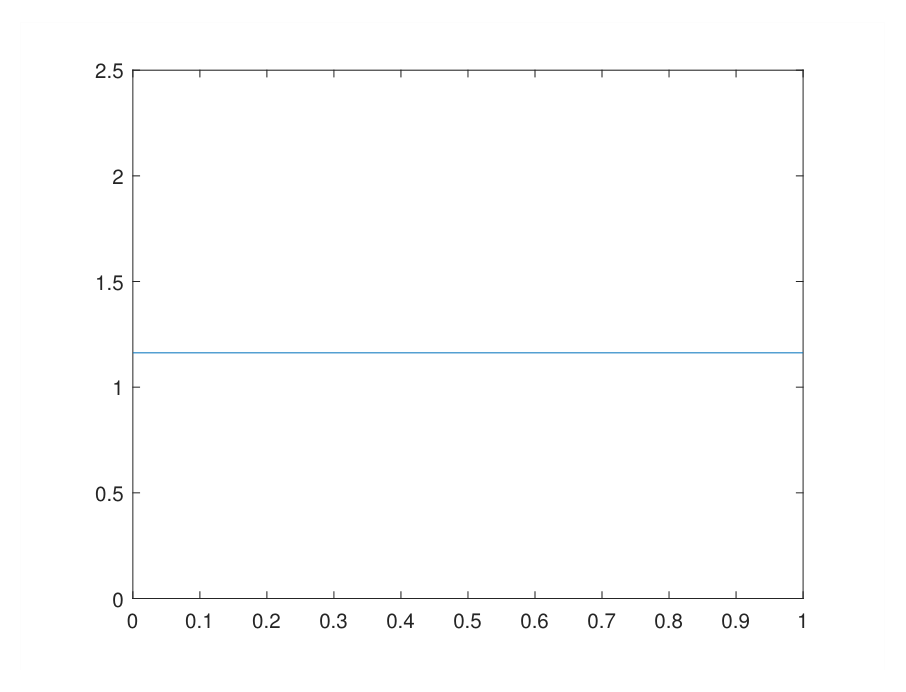
\[\begin{aligned} \frac{\partial^2 J_3(x)}{\partial x^2}=&\frac{10^{14}}{K^3}\cos\left(\frac{K^4}{x/10^{10}+K}\right)\;\left(\frac{-K^4}{(x/10^{10}+K)^2}\right)^2\left(\frac{1}{10^{10}}\right)^2 \nonumber \\ &+2\frac{10^{14}}{K^3}\sin\left(\frac{K^4}{x/10^{10}+K}\right)\;\left(\frac{K^4}{(x/10^{10}+K)^3}\right)\left(\frac{1}{10^{10}}\right)^2, \end{aligned}\tag{52}\] respectively.
For their graphs, please see Figures 1 and 2, repectively.
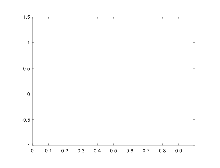
Thus, with the results of the previous section in mind, we may obtain \[\begin{aligned} \frac{\partial J_5(u)}{\partial u}=&\frac{\partial J(u)}{\partial u} +\frac{\partial J_3(u)}{\partial u} = \frac{\partial J(u)}{\partial u}+\mathcal{O}\left(0.003\right). \end{aligned}\tag{53}\]
Moreover, \[\begin{aligned} \frac{\partial^2 J_5(u)}{\partial u^2}=&\frac{\partial^2 J(u)}{\partial u^2}+\frac{\partial^2 J_3(u)}{\partial u^2} = \frac{\partial^2 J(u)}{\partial u^2}+\mathcal{O}\left(1.16\right) > \mathbf{0}, \text{ in } V_1. \end{aligned}\tag{54}\]
Observe that \(J_5\) is convex and its first variation has a very small perturbation concerning the original first variation of \(J\).
For a initial solution \(u_0\equiv 0.1, \text{ in } [0,1],\) we shall apply the Newton’s Method with a grid of 100 nodes in a finite differences context, for the interval \([0,1].\) For standard results on the finite differences method, please see [21].
For the approximate functional \(J_5\), the Newton’s method iterations stand for \[(u_1)_{n+1}=(u_1)_n-[J_5”((u_1)_n)]^{-1} (J_5′(u_1)_n).\]
On the other hand, the iterations for the Newton’s Method for \(J\), stand for \[(u_2)_{n+1}=(u_2)_n-[J”((u_2)_n)]^{-1} (J'(u_2)_n),\] where generically, \(u_1\) denotes the solution for the approximate problem and \(u_2\) the solution for the original one.
Here we present tables with the concerning iterations.
For the approximate problem related to the functional \(J_5\), please see Table 1.
For the original problem related to the functional \(J\), please see Table 2.
| iteration \(k\) | \(u_1(0.5)\) |
|---|---|
| 1 | 1.1604 |
| 2 | 1.1436 |
| 3 | 1.1443 |
| 4 | 1.1450 |
| 5 | 1.1453 |
| 6 | 1.1453 |
| iteration \(k\) | \(u_2(0.5)\) |
|---|---|
| 1 | 75.5311 |
| 2 | 50.3542 |
| 3 | 33.5697 |
| 4 | 22.3802 |
| 5 | 14.9210 |
| 6 | 9.9491 |
| 7 | 6.6365 |
| 8 | 4.4327 |
| 9 | 2.9745 |
| 10 | 2.0300 |
| 11 | 1.4663 |
| 12 | 1.2080 |
| 13 | 1.1493 |
| 14 | 1.1464 |
| 15 | 1.1464 |
For the graphs obtained for the solutions \(u_1\) e \(u_2\), please see Figures 3 and 4, respectively.
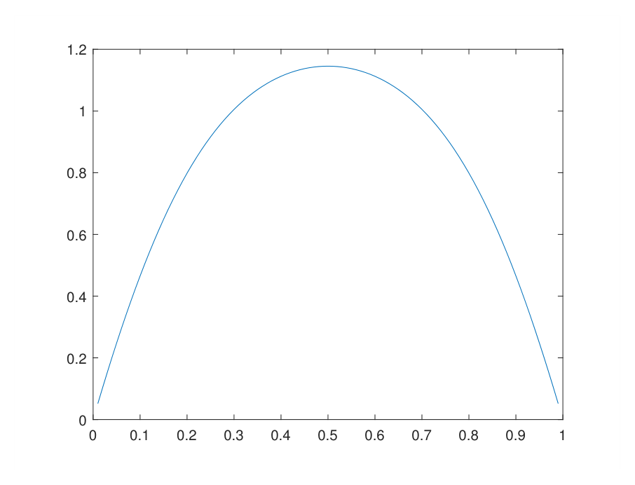
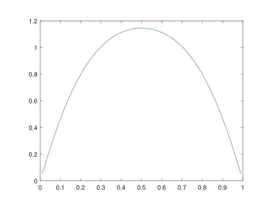
Looking at Tables 1 and 2, we may see that the approximate solution \(u_1\), related to the functional \(J_5\), converged in \(5\) iterations, whereas solution \(u_2\), related to the original functional \(J\), converged in \(14\) iterations.
Therefore, the convergence for the convex approximate model is considerably faster, as expected.
Finally, here we present the software in MAT-LAB through which such results were obtained:
clear all
m8=100;
d=1/m8;
A=1;
B=1;
e1=0.1;
\(K=500000*2*\pi;\)
yo=ones(m8-1,1);
m2=zeros(m8-1,m8-1);
for i=2:m8-2
m2(i,i)=-2.0;
m2(i,i+1)=1.0;
m2(i,i-1)=1.0;
end;
m2(1,1)=-2.0;
m2(1,2)=1.0;
m2(m8-1,m8-1)=-2.0;
m2(m8-1,m8-2)=1.0;
Id=eye(m8-1);
for i=1:m8-1
uo(i,1)=0.1;
end;
k1=1;
b12=1.0;
while \((b12>10^{-4})\) && \((k1<100)\)
k1
k1=k1+1;
for i=1:m8-1
\(F1(i,1)=10^{14}/K^3*sin(K^4/(uo(i,1)/10^{10}+K))*(-K^4)/(uo(i,1)/10^{10}+K)^2*1/10^{10};\)
\(F2(i,1)=10^{14}/K^3*cos(K^4/(uo(i,1)/10^{10}+K))\\ *((-K^4)/(uo(i,1)/10^{10}+K)^2)^2*(1/10^{10})^2;\)
\(F2(i,1)=F2(i,1) \\ +2*10^{14}/K^3*sin(K^4/(uo(i,1)/10^{10}+K))*(K^4)/(uo(i,1)/10^{10}+K)^3*(1/10^{10})^2;\)
end;
\(M=-e1*m2/d^2+diag(3*uo(:,1).*uo(:,1))*A-B*Id+diag(F2(:,1));\)
\(u1=uo-inv(M)*(-e1*m2/d^2*uo(:,1)-yo(:,1) \\ +uo(:,1).*uo(:,1).*uo(:,1)*A-B*uo(:,1)+F1(:,1));\)
b12=max(abs(u1-uo));
uo=u1;
u11(k1-1)=uo(m8/2,1);
end;
for i=1:m8-1
uo(i,1)=0.1;
end;
k=1;
b14=1.0;
while \((b14>10^{-4})\) && \((k<100)\)
k
k=k+1;
\(M=-e1*m2/d^2+diag(3*uo(:,1).*uo(:,1))*A-B*Id;\)
\(u2=uo-inv(M)*(-e1*m2/d^2*uo(:,1)-yo(:,1)\\ +uo(:,1).*uo(:,1).*uo(:,1)*A-B*uo(:,1));\)
b14=max(abs(u2-uo));
uo=u2;
u12(k-1)=uo(m8/2,1);
end;
for i=1:m8-1
x1(i,1)=i*d;
end;
plot(x1,u1);
The objective of this section is complete.
Let \(\Omega \subset \mathbb{R}^3\) be an open, bounded and connected set with a regular (Lipschitzian) boundary denoted by \(\partial \Omega.\)
Consider a functional \(J:V \rightarrow \mathbb{R}\) defined by
\[J(u)=F(\Lambda u)-\langle u,f \rangle_V,\] where \(V=W_0^{1,2}(\Omega; \mathbb{R}^N).\)
Moreover, denoting \(Y=Y^*=L^2(\Omega;\mathbb{R}^N)\), \(Y_1=Y_1^*=L^2(\Omega;\mathbb{R}^m)\), \(F:Y \rightarrow \mathbb{R}\) is such that \[F(\Lambda u)=\frac{1}{2}\int_\Omega \min_{k \in \{1,\cdots, M\}} g_k(\Lambda u)\;dx.\]
Here, \(g_k:\mathbb{R}^m \rightarrow \mathbb{R}\) is a twice differentiable convex function, \(\forall k \in \{1, \cdots, M\},\) for some \(M \in \mathbb{N}.\)
Also, \(f \in Y^*\) and \(\Lambda :V \rightarrow Y_1\) is a bounded and linear operator whose the adjoint one is denoted by \(\Lambda^*:Y_1^* \rightarrow V^*.\)
Observe that \[\begin{aligned} J(u)=& F(\Lambda u)-\langle u,f \rangle_V \nonumber \\ =& -\langle \Lambda u,v^* \rangle_{L^2}+F(\Lambda u) + \langle \Lambda u,v^* \rangle_{L^2}-\langle u,f \rangle_V \nonumber \\ \geq& \inf_{ v \in Y_1} \{-\langle v,v^* \rangle_{L^2}+F(v) \} +\inf_{ u \in V}\{ \langle \Lambda u,v^* \rangle_{L^2}-\langle u,f \rangle_V\} \nonumber \\ =& -F^*(v^*), \end{aligned}\tag{55}\] \(\forall v^* \in A^*\), where \[A^*=\{ v^* \in Y_1^*\;:\; \Lambda^* v^*-f=\mathbf{0}\}.\]
Observe also that \[\begin{aligned} \inf_{ v \in Y_1} \{-\langle v,v^* \rangle_{L^2}+F(v) \} =& \inf_{ v \in Y_1} \left\{-\langle v,v^* \rangle_{L^2}+\frac{1}{2}\int_\Omega \min_{k \in \{1, \cdots,M\}} g_k(v)\;dx \right\} \nonumber \\ =& \int_\Omega \left(\min_{k \in \{1,\cdots, M\}} \left\{\inf_{ v \in Y_1} \{ -v v^*+g_k(v)\}\right\}\right)\;dx \nonumber \\ =& \int_\Omega \min_{k \in \{1,\cdots, M\}}(- g_k^*(v^*))\;dx \nonumber \\ =& -\int_\Omega \max_{k \in \{1,\cdots, M\}} g_k^*(v^*)\;dx \nonumber \\ =& -F^*(v^*). \end{aligned}\tag{56}\]
In summary, we have got, \[\begin{aligned} \inf_{ u \in V} J(u) \geq& \inf_{u \in V} \{F^{**}(\Lambda u)-\langle u,f \rangle_V\} \nonumber \\ =& \sup_{ v^* \in A^*}\{-F^*(v^*)\}. \end{aligned}\tag{57}\]
The dual problem is concave and has a solution \((u_0,v_0^*)\) where \(u_0 \in V\) is an appropriate Lagrange multiplier for the Lagrangian \[\begin{aligned} L(v^*,u)=&F^*(v^*)-\langle u, \Lambda^*v^*-f\rangle_V \nonumber \\ =&F^*(v^*)-\langle \Lambda u,v^* \rangle_{L^2}+\langle u,f \rangle_V, \end{aligned}\tag{58}\] so that the following extremal equations are satisfied \[\Lambda u_0 = \partial F^*(v_0^*),\] and \[\Lambda^*v_0^*-f= \mathbf{0}.\]
Hence, \[v_0^* \in \partial F^{**}(\Lambda u_0),\] \[\begin{aligned} F^*(v_0^*)=& \langle \Lambda u_0,v_0^*\rangle_{L^2}-F^{**}(\Lambda u_0) \nonumber \\ =& \langle u_0, \Lambda^*v^* \rangle_V-F^{**}(u_0), \end{aligned}\tag{59}\] and thus, \[F^{**}(u_0)-\langle u,f \rangle_{L^2}=-F^*(v_0^*),\] so that \[\begin{aligned} J(u_0)=&F(\Lambda u_0)-\langle u_0, f \rangle_V \nonumber \\ \geq& F^{**}(\Lambda u_0)-\langle u_0,f \rangle_V \nonumber \\ =&\inf_{u \in V} \{F^{**}(\Lambda u)-\langle u,f \rangle_V\} \nonumber \\ =& \sup_{ v^* \in A^*}\{-F^*(v^*)\} \nonumber \\ =& -F^*(v_0^*). \end{aligned}\tag{60}\]
Observe that an optimal point may not be attained, so that it remains still the issue of obtaining an appropriate critical point for \(J\) at least close to optimal.
Having obtained such a \(u_0 \in V\) which minimizes the relaxed functional \[F^{**}(u)-\langle u,f \rangle_{V},\] we shall propose a procedure for obtaining such a appropriate \(\hat{u}_0\) close to optimal for \(J.\)
We start by defining the functionals \(F_1:V \rightarrow \mathbb{R}\) and \(F_2:V \rightarrow \mathbb{R}\), by \[F_1(u)=F(\Lambda u)+\frac{K}{2}\int_\Omega |u-u_0|^2\;dx-\langle u,f\rangle_V,\] and \[F_2(u)=\frac{K}{2}\int_\Omega |u-u_0|^2\;dx,\] so that \[J(u)=F_1(u)-F_2(u).\]
Moreover, we define \(F_1^*:Y^* \rightarrow \mathbb{R}\) and \(F_2^*:Y^* \rightarrow \mathbb{R}\), by \[F_1^*(z^*)=\sup_{ u \in V}\{\langle u-u_0,z^* \rangle_{L^2}-F_1(u)\},\] and \[\begin{aligned} F_2^*(z^*)=&\sup_{ v \in Y}\{\langle v-u_0,z^* \rangle_{L^2}-F_2(v)\} \nonumber \\ =& \frac{1}{2 K}\int_\Omega |z^*|^2\;dx. \end{aligned}\tag{61}\]
Observe that \[\begin{aligned} J(u)=&F_1(u)-F_2(u) \nonumber \\ =& -\langle u-u_0,z^* \rangle_{L^2}+F_1(u) +\langle u-u_0,z^* \rangle_{L^2}-F_2(u) \nonumber \\ \leq& -\langle u-u_0,z^* \rangle_{L^2}+F_1(u)+\sup_{ v \in Y}\{\langle v-u_0,z^* \rangle_{L^2}-F_2(v)\} \nonumber \\ =& F_1(u)-\langle u-u_0,z^* \rangle_{L^2}+F_2^*(z^*), \end{aligned}\tag{62}\] \(\forall u \in V,\; z^* \in Y^*.\)
Let \(\alpha_1 \in \mathbb{R}\) be such that \[\alpha_1=\inf_{ u \in V} J(u).\]
From the last previous lines we have got \[\begin{aligned} \alpha_1 =& \inf_{u \in V} J(u) \nonumber \\ \leq& \inf_{ u \in V}\{F_1(u)-\langle u-u_0,z^* \rangle_{L^2}\}+F_2^*(z^*) \nonumber \\ =& -F_1^*(z^*)+F_2^*(z^*), \end{aligned}\tag{63}\] \(\forall z^* \in Y^*\).
Therefore \[\begin{aligned} \alpha_1 =& \inf_{u \in V} J(u) \nonumber \\ \leq& \inf_{z^* \in Y^*}\{ -F_1^*(z^*)+F_2^*(z^*)\}. \end{aligned}\tag{64}\]
Indeed, from the general results in Toland [5], we may obtain \[\begin{aligned} \alpha_1 =& \inf_{u \in V} J(u) \nonumber \\ =& \inf_{z^* \in Y^*}\{ -F_1^*(z^*)+F_2^*(z^*)\}. \end{aligned}\tag{65}\] so that \[\begin{aligned} \alpha_1 =& \inf_{u \in V} J(u) \nonumber \\ =& \inf_{z^* \in Y^*}\{ -F_1^*(z^*)+F_2^*(z^*)\} \nonumber \\ =& \inf_{(u,z^*) \in V \times Y^*}\{F_1(u)-\langle u-u_0,z^* \rangle_{L^2}+F_2^*(z^*)\}. \end{aligned}\tag{66}\]
Defining \(J_8:V \times Y^* \rightarrow \mathbb{R}\) by \[J_8(u,z^*)=F_1(u)-\langle u-u_0,z^* \rangle_{L^2}+F_2^*(z^*),\] we have got \[\begin{aligned} \alpha_1 =& \inf_{u \in V} J(u) \nonumber \\ =& \inf_{z^* \in Y^*}\{ -F_1^*(z^*)+F_2^*(z^*)\} \nonumber \\ =& \inf_{(u,z^*) \in V \times Y^*}\{J_8(u,z^*)\}. \end{aligned}\tag{67}\]
For a very large value for \(K>0\) we shall propose to obtain an appropriate critical point for \(J\), through obtaining a critical point of \(J_8\) intended to be close to optimal.
In the next subsection we present some numerical examples for related models.
In this subsection we develop duality principles for some models in phase transition. Similar results and models are addressed in [22].
Let \(\Omega=[0,1] \subset \mathbb{R},\) and consider a functional \(J:V \rightarrow \mathbb{R}\) defined by \[J(u)= \frac{1}{2}\int_\Omega \min\{(u’-1)^2,(u’+1)^2\}\;dx+\frac{1}{2} \int_\Omega (u-f)^2\;dx,\] where \[V=\{ u \in W^{1,2}(\Omega)\;:\; u(0)=0 \text{ and } u(1)=1/2\}.\]
In this subsection, we also denote \[Y=Y^*=L^2(\Omega).\]
Observe that \[\begin{aligned} J(u)=& -\langle u’,v^* \rangle_{L^2}+\frac{1}{2}\int_\Omega \min\{(u’-1)^2,(u’+1)^2\}\;dx +\langle u’,v^* \rangle_{L^2}+\frac{1}{2}\int_\Omega (u-f)^2\;dx \nonumber \\ \geq& \inf_{ v \in Y}\left\{-\langle v,v^* \rangle_{L^2}+\frac{1}{2}\int_\Omega \min\{(v-1)^2,(v+1)^2\}\;dx\right\} +\inf_{u \in V}\left\{\langle u’,v^* \rangle_{L^2}+\frac{1}{2}\int_\Omega (u-f)^2\;dx\right\} \nonumber \\ =& -\int_\Omega \max\left\{ \frac{1}{2}(v^*)^2+v^*, \frac{1}{2}(v^*)^2-v^*\right\}\;dx -\frac{1}{2}\int_\Omega ((v^*)’+f)^2\;dx -v^*(1) u(1) \nonumber \\ =&-\frac{1}{2}\int_\Omega (v^*)^2\;dx-\int_\Omega |v^*|\;dx -\frac{1}{2}\int_\Omega ((v^*)’+f)^2\;dx +v^*(1) u(1). \end{aligned}\tag{68}\]
Defining \[\begin{aligned} J^*(v^*)=& -\frac{1}{2}\int_\Omega (v^*)^2\;dx-\int_\Omega |v^*|\;dx-\frac{1}{2}\int_\Omega ((v^*)’+f)^2\;dx +v^*(1) u(1). \end{aligned}\tag{69}\] we have obtained \[\inf_{u \in V} J(u) \geq \sup_{v^* \in Y^*}J^*(v^*).\]
Indeed, from standard results on basic convex analysis for such a scalar case, we have \[\inf_{u \in V} J(u) = \sup_{v^* \in Y^*}J^*(v^*).\]
We have obtained numerical results concerning the maximization of \(J^*\) for the cases \(A\) and \(B\), where
Case \(A\): \(f(x)=\sin(\pi x)/2,\)
Case \(B\): \(f(x)\equiv 0, \text{ on } [0,1].\)
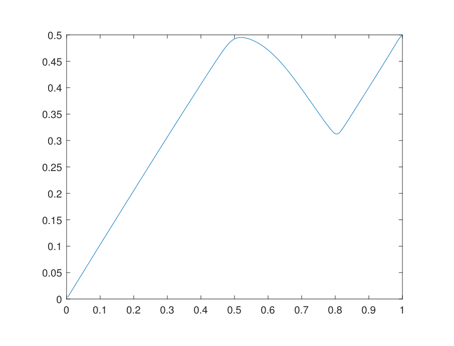
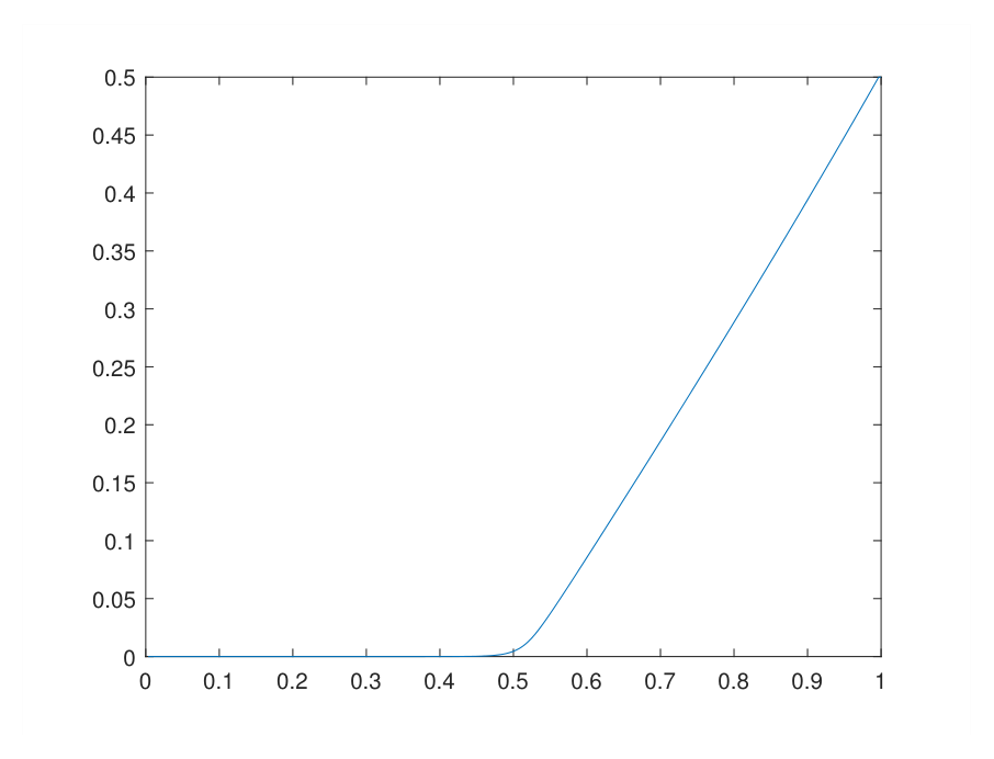
For the corresponding graphs for the optimal solutions \[u_0=(v^*_0)’+f,\] obtained, please see Figures 5 and 6, respectively.
The results were obtained through the first part of software presented at the end of this subsection.
Consider now a closely related functional \(J_1:V \rightarrow \mathbb{R},\) where \[J_1(u)=\frac{1}{2}\int_\Omega ((u’)^2-1)^2\;dx+\frac{1}{2}\int_\Omega(u-f)^2\;dx.\]
It is well known from the current literature that a global minimum for \(J_1\) may not be attained.
Having obtained such a previous solution \(u_0 \in V\) of the closely related functional \(J\), which has critical points close to those of \(J_1\), we shall present a procedure to obtain a critical point for \(J_1\) intended to be approximately optimal.
Define the functionals \(F_1:V \rightarrow \mathbb{R}\) and \(F_2:V \rightarrow \mathbb{R}\) by
\[F_1(u)=\frac{1}{2}\int_\Omega ((u’)^2-1)^2\;dx+\frac{K}{2}\int_\Omega (u-u_0)^2\;dx+\frac{1}{2}\int_\Omega (u-f)^2\;dx,\] and \[F_2(u)=\frac{K}{2}\int_\Omega(u-u_0)^2\;dx,\] so that \[\begin{aligned} J_1(u)=& F_1(u)-F_2(u) \nonumber \\ =& -\langle u-u_0,z^*\rangle_{L^2}+F_1(u) +\langle u-u_0,z^*\rangle_{L^2}-F_2(u) \nonumber \\ \leq& -\langle u-u_0,z^*\rangle_{L^2}+F_1(u) +\sup_{ v \in Y}\{\langle v-u_0,z^*\rangle_{L^2}-F_2(v)\} \nonumber \\ =& F_1(u)-\langle u-u_0,z^*\rangle_{L^2}+F_2^*(z^*) \nonumber \\ =& J_3(u,z^*). \end{aligned}\tag{70}\]
Observed that clearly \[\inf_{u \in V} J_1(u)=\inf_{(u,z^*) \in V \times Y^*} J_3(u,z^*).\]
Therefore, for a large value of \(K>0\), we shall obtain an appropriate critical point of \(J_1\), by obtaining a critical point of \(J_3\), intended to be approximately optimal for \(J_1\), through the following algorithm.
Set \(n=1\), \(K=3000000\), \(0<\varepsilon \ll 1\) (small) and \(z_n^*\equiv 0.\)
Find \(u_n \in V\) such that \[\frac{\partial J_3(u_n,z^*_n)}{\partial u}=\mathbf{0}.\]
Find \(z_{n+1}^* \in Y^*\) such that \[\frac{\partial J_3(u_n,z^*_{n+1})}{\partial z^*}=\mathbf{0},\] so that \[z^*_{n+1}=K(u_n-u_0).\]
If \(\|z^*_{n+1}-z^*_n\|_\infty\leq \varepsilon\), then stop. Otherwise \(n:=n+1\) and go to item 2.
We have obtained solutions for the cases \(C\) and \(D\).
Case \(C\), for \(f(x)=\sin(\pi x)/2\) and \(u_0\) of Case \(A\) of the previous section.
Case \(D\), for \(f(x)\equiv 0\) and \(u_0\) obtained in Case \(B\) of the previous section.
For the corresponding graphs obtained for the solutions \(\hat{u}\), please see Figures 7 and 8, respectively.
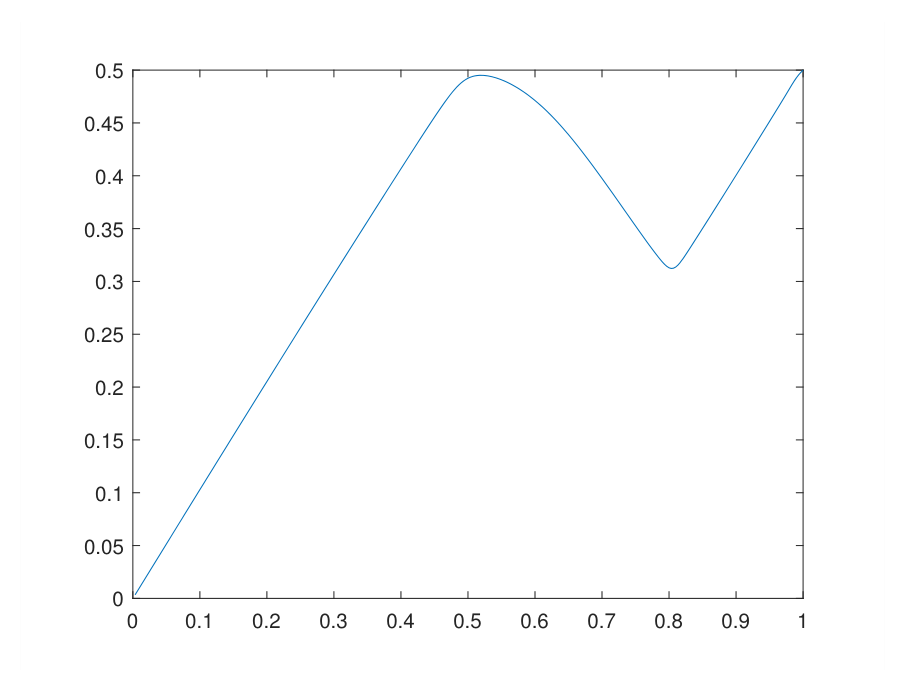
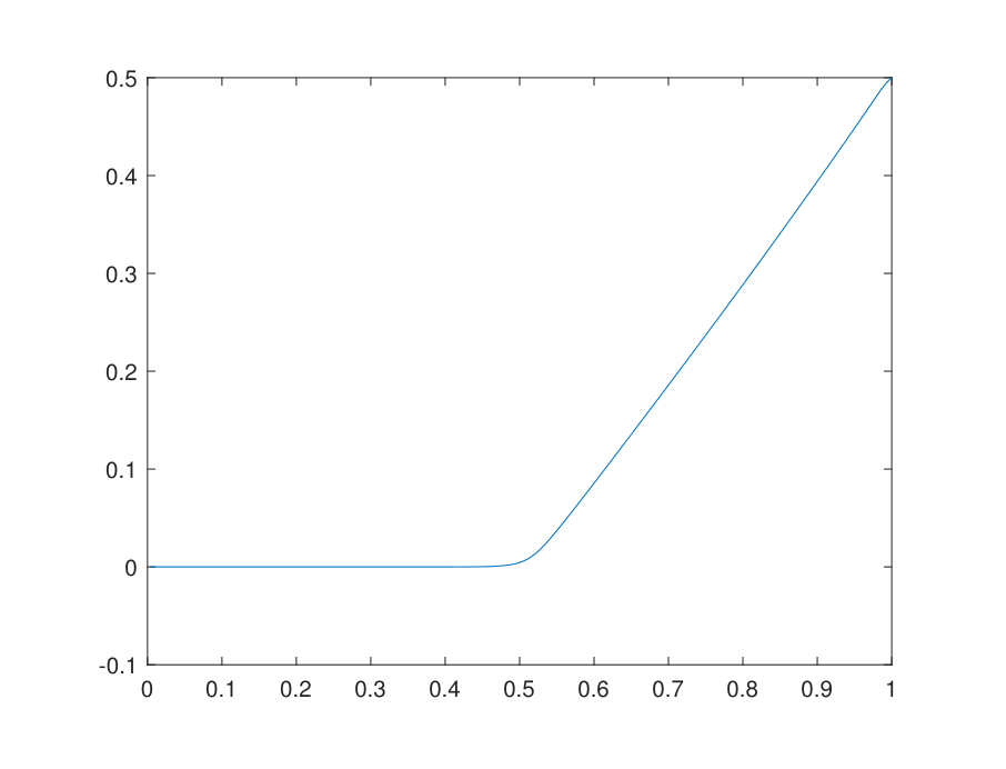
Remark 3. Observe that figures for the Cases \(A\) and \(C\) and, \(B\) and \(D\) respectively, are very similar, as expected since it is well known in the literature the functionals \(J\) and \(J_1\) have in general very close critical points.
Here we present the software in MAT-LAB through which such results have been obtained.
clear all
global m8 d yo K e1 u z1 u3 e3
m8=300;
d=1/m8;
e3=0.0000001;
K=3000000;
e1=0.0001;
for i=1:m8
yo(i,1)=sin(i*d*pi)/2*0;
z1(i,1)=0.0;
end;
for i=1:m8-1
y1(i,1)=(yo(i+1,1)-yo(i,1))/d;
end;
vo(:,1)=0.1*ones(m8,1);
b12=1.0;
k=1;
while \((b12>10^{-4})\) && \((k<100)\)
k
k=k+1;
for i=1:m8
\(wo(i,1)=\sqrt{vo(i,1)^2+e3};\)
end;
i=1;
\(m12=1+d^2/wo(i,1)+d^2;\)
m50(i)=1/m12;
\(z(i)=m50(i)*(y1(i,1)*d^2+yo(i,1)*d);\)
for i=2:m8-1
\(m12=2+d^2/wo(i,1)+d^2-m50(i-1);\)
m50(i)=1/m12;
\(z(i)=m50(i)*(y1(i,1)*d^2+z(i-1));\)
end;
v(m8,1)=1/(1-m50(m8-1))*(d/2-d*yo(m8,1)+z(m8-1));
for i=1:m8-1
v(m8-i,1)=m50(m8-i)*v(m8-i+1,1)+z(m8-i);
end;
b12=max(abs(v-vo));
vo=v;
for i=1:m8-1
u(i,1)=(vo(i+1,1)-vo(i,1))/d+yo(i+1,1);
end;
u(m8,1)=1/2;
u(m8/2,1)
end;
u3=u;
xo=u3;
x1=u3;
b14=1;
k1=1;
while \((b14>10^{-4})\) && \((k1<100)\)
k1
k1=k1+1;
b12=1;
k=1;
while \((b12>10^{-4})\) && \((k<100)\)
k
k=k+1;
X=fminunc(’funsep20244’,xo);
b12=max(abs(X-xo));
xo=X;
u(m8/2,1)
end;
z1=K*(u-u3);
b14=max(abs(x1-xo));
x1=xo;
end;
for i=1:m8
x5(i,1)=i*d;
end;
plot(x5,u);
***********************
With the auxiliary function “funsep20244”
*************************************
function S=funsep20244(x)
global m8 d yo K e1 u z1 u3 e3
for i=1:m8
u(i,1)=x(i,1);
end;
u(m8,1)=1/2;
du(1,1)=u(1,1)/d;
for i=2:m8
du(i,1)=(u(i,1)-u(i-1,1))/d;
end;
\(d2u(1,1)=(-2*u(1,1)+u(2,1))/d^2;\)
for i=2:m8-1
\(d2u(i,1)=(u(i+1,1)-2*u(i,1)+u(i-1,1))/d^2;\)
end;
S=0;
for i=1:m8
\(S=S+1/2*(du(i,1)^2-1)^2+1/2*(u(i,1)-yo(i,1))^2+K*(u(i,1)-u3(i,1))^2/2;\)
S=S-z1(i,1)*(u(i,1)-u3(i,1));
end;
for i=1:m8-1
\(S=S+e1*d2u(i,1)^2;\)
end;
*****************************************
Let \(\Omega \subset \mathbb{R}^n\) be an open, bounded and connected set with a regular (Lipschitzian) boundary denoted by \(\partial \Omega.\)
Consider a functional \(J:V \rightarrow \mathbb{R}\) defined by
\[J(u)=F(\nabla u)-\langle u,f \rangle_{L^2},\] where \(V=W_0^{1,2}(\Omega; \mathbb{R}^N).\)
Moreover, denoting \(Y=Y^*=L^2(\Omega;\mathbb{R}^N)\), \(Y_1=Y_1^*=L^2(\Omega;\mathbb{R}^{Nn})\), assume \(F:Y_1 \rightarrow \mathbb{R}\) is such that \[F(\nabla u)=\int_\Omega \min_{k \in \{1,\cdots, M\}} g_k(\nabla u)\;dx.\]
Here, \(g_k:\mathbb{R}^{Nn} \rightarrow \mathbb{R}\) is a twice differentiable convex function, \(\forall k \in \{1, \cdots, M\},\) for some \(M \in \mathbb{N}.\)
Also, \(f \in Y^*\) and \(\nabla :V \rightarrow Y_1\) is a bounded and linear operator whose the adjoint one is denoted by \(-\text{ div }:Y_1^* \rightarrow V^*.\)
Observe that defining \[B=\left\{\{t_k\} \text{ measurable }\;:\; 0 \leq t_k \leq 1, \; \forall k \in \{1, \cdots, M\} \text{ and } \sum_{k=1}^Mt_k=1, \text{ in } \Omega\right\},\] we have \[F(\nabla u)=\inf_{t \in B} \left\{\int_\Omega \left(\sum_{k=1}^M t_k g_k(\nabla u)\right)\;dx\right\}.\]
Here we define \(F_1: Y_1 \times B \rightarrow \mathbb{R}\) and \(J_1: V \times B \rightarrow \mathbb{R}\), by
\[F_1(\nabla u,t)=\int_\Omega \left(\sum_{k=1}^M t_k g_k(\nabla u)\right)\;dx,\] and \[J_1(u,t)=F_1(\nabla u,t)-\langle u,f \rangle_{L^2}.\]
Observe that \[\begin{aligned} J(u)=& F(\nabla u)-\langle u,f \rangle_{L^2} \nonumber \\ =& \inf_{t \in B} \left\{\int_\Omega \left(\sum_{k=1}^M t_k g_k(\nabla u)\right)\;dx\right\} -\langle u,f \rangle_{L^2} \nonumber \\ =& -\langle \nabla u,v^*\rangle_{L^2}+\inf_{t \in B} \left\{\int_\Omega \left(\sum_{k=1}^M t_k g_k(\nabla u)\right)\;dx\right\} +\langle \nabla u,v^*\rangle_{L^2}-\langle u,f \rangle_{L^2} \nonumber \\ \geq& \inf_{v \in Y_1}\left\{-\langle v,v^*\rangle_{L^2}+\inf_{t \in B} \left\{\int_\Omega \left(\sum_{k=1}^M t_k g_k(v)\right)\;dx\right\} \right\}+\inf_{ u \in V}\left\{ -\langle u, \text{ div }v^* \rangle_{L^2}-\langle u,f \rangle_{L^2}\right\} \nonumber \\ =& \inf_{t \in B}\left\{\inf_{v \in Y_1}\left\{-\langle v,v^*\rangle_{L^2}+\int_\Omega \left(\sum_{k=1}^M t_k g_k(v)\right)\;dx\right\} \right\}+\inf_{ u \in V}\left\{ -\langle u,\text{ div }v^* \rangle_{L^2}-\langle u,f \rangle_{L^2}\right\} \nonumber \\ =& \inf_{t \in B}\int_\Omega \left(-\left(\sum_{k=1}^M t_kg_k\right)^*(v^*)\right)\;dx+\inf_{ u \in V}\left\{ -\langle u,\text{ div }v^* \rangle_{L^2}-\langle u,f \rangle_{L^2}\right\} \nonumber \\ =& \inf_{t \in B}\left(-\int_\Omega \left(\sum_{k=1}^M t_k g_k\right)^*(v^*)\;dx\right), \end{aligned}\tag{71}\] \(\forall v^* \in A^*\), where \[A^*=\{ v^* \in Y_1^*\;:\; \text{ div } v_j^*+f_j=\mathbf{0},\; \text{ in } \Omega,\; \forall j \in \{1,\cdots, N\}\}.\]
In summary, denoting \(F^*:Y_1^*\times B \rightarrow \mathbb{R}\) by \[F^*(v^*,t)=\int_\Omega \left(\sum_{k=1}^M t_kg_k\right)^*(v^*)\;dx,\] we have got \[\begin{aligned} \inf_{ u \in V} J(u)=& \inf_{(u,t) \in V \times B}J_1(u,t) \nonumber \\ \geq& \sup_{ v^* \in A^*}\left\{\inf_{t \in B}\{-F^*(v^*,t)\}\right\}. \end{aligned}\tag{72}\]
Observe also that, fixing \(t \in B\), from standard results on convex analysis, we have \[\inf_{u \in V} J_1(u,t)=\sup_{ v^* \in A^*}\{-F^*(v^*,t)\},\] so that \[\inf_{(u,t) \in V \times B}J_1(u,t)= \inf_{ t \in B}\left\{ \sup_{ v^* \in A^*}\{-F^*(v^*,t)\}\right\},\]
Thus, we have obtained \[\begin{aligned} \inf_{ u \in V} J(u)=& \inf_{(u,t) \in V \times B}J_1(u,t) \nonumber \\ =& \inf_{ t \in B}\left\{ \sup_{ v^* \in A^*}\{-F^*(v^*,t)\}\right\} \nonumber \\ \geq& \sup_{ v^* \in A^*}\left\{\inf_{t \in B}\{-F^*(v^*,t)\}\right\}. \end{aligned}\tag{73}\]
Recall that the restriction defining \(B\) is equivalent to \[t_k^2-t_k \leq 0, \forall k \in \{1, \cdots,M\},\] and \[\sum_{k=1}^M t_k=1, \text{ in } \Omega.\]
Thus, already including the Lagrange multipliers for the concerning restrictions, define now the Lagrangian \[L(v^*,t,u,\lambda)=-F^*(v^*,t)-\langle u, \text{ div } v^*+f\rangle_{L^2}+\sum_{k=1}^M\langle\lambda_k^2,t_k^2-t_k\rangle_{L^2} +\left\langle \lambda_0, \sum_{k=1}^M t_k-1\right\rangle_{L^2}.\]
Let \[(\hat{v}^*, t_0,u_0, \hat{\lambda}) \in Y_1^* \times B \times V \times L^2(\Omega; \mathbb{R}^{M+1}),\] be such that \[\delta L(\hat{v}^*,t_0,u_0,\hat{\lambda})=\mathbf{0}.\]
From evident convexity \[-F^*(\hat{v}^*,t_0)=\sup_{ v^* \in A^*}\{-F^*(v^*,t_0)\}.\]
Suppose such a \(t_0 \in B\) is such that \[-F^*(\hat{v}^*,t_0)=\inf_{ t \in B}\{-F^*(\hat{v}^*,t)\}.\]
In summary, we have got \[\begin{aligned} -F^*(\hat{v}^*,t_0)=&\inf_{ t \in B}\{-F^*(\hat{v}^*,t)\} \nonumber \\ =& \sup_{ v^* \in A^*}\{-F^*(v^*,t_0)\}. \end{aligned}\tag{74}\]
From such results and a standard Saddle Point Theorem we may infer that \[\begin{aligned} -F^*(\hat{v}^*,t_0)=&\inf_{ t \in B}\left\{\sup_{ v^* \in A^*}\{-F^*(v^*,t)\}\right\} \nonumber \\ =& \sup_{ v^* \in A^*}\left\{ \inf_{t \in B} \{-F^*(v^*,t)\}\right\}. \end{aligned}\tag{75}\]
Moreover from the extremal equation \[\nabla u_0 =\frac{ \partial F^*(\hat{v}^*,t_0)}{\partial v^*},\] we obtain \[F^*(\hat{v}^*,t_0)=\langle \nabla u_0, \hat{v}^*\rangle_{L^2}-F_1(u_0,t_0),\] that is, \[F^*(\hat{v}^*,t_0)=\langle u_0,-\text{ div }\hat{v}^*\rangle_{L^2}-F_1(u_0,t_0),\] so that \[F^*(\hat{v}^*,t_0)=\langle u_0,f \rangle_{L^2}-F_1(u_0,t_0),\] so that \[J_1(u_0,t_0)=-F^*(\hat{v}^*,t_0).\]
Joining the pieces, we have got \[\begin{aligned} J(u_0)=&\inf_{u \in V} J(u) \nonumber \\ =& \inf_{(u,t) \in V \times B} J_1(u,t) \nonumber \\ =& J_1(u_0,t_0) \nonumber \\ =& -F^*(\hat{v}^*,t_0) \nonumber \\ =&\inf_{ t \in B}\left\{\sup_{ v^* \in A^*}\{-F^*(v^*,t)\}\right\} \nonumber \\ =& \sup_{ v^* \in A^*}\left\{ \inf_{t \in B} \{-F^*(v^*,t)\}\right\}. \end{aligned}\tag{76}\]
Remark 4. A concerning issue here is that the infimum in \(t \in B\) for \(-F^*(\hat{v}^*,t)\) may not be attained considering that such a functional is non convex in \(t\). However, similarly as for the Ekeland variational principle, we obtain a \(t_0 \in B\) close to optimal and approximately satisfying the related Euler-Lagrange equations for \(L\). In such a case, in (76) we would obtain only the approximations \[J(u_0)\approx \inf_{u \in V}J(u)=\inf_{(u,t) \in V \times B} J_1(u,v)\approx J_1(u_0,t_0)\approx -F_1^*(\hat{v}^*,t_0).\]
That is the case as the global minimum is not attained for \(J\). However, we emphasise that for a finite dimensional model version, in a finite differences or finite elements context, such mentioned extremals are always attained so that, in such a case, (76) holds. We emphasize this exact solutions obtained for such approximate finite dimensional models represent points close to optimal for the originally non-convex functional \(J\) defined in an infinite dimensional function space.
The objective of this section is complete.
In this article, we have developed duality principles and related convex dual variational formulations for originally non-convex primal ones. As a first application, we have set duality principles and respective convex dual formulations for a Ginzburg-Landau model in superconductivity. In the final sections we have addressed related models in phase transition.
We highlight the results here obtained are applicable to a large class of models in the calculus of variations, including some plate and shell non-linear theories, other models in superconductivity, phase transition and micro-magnetism, among many others.
In a near future research we intend to apply such results to some of these mentioned related models.