On integrable SLIR epidemic model

1. Introduction

Compartmental mathematical models for studying epidemiological dynamics have been used since Daniel Bernoulli in 1760 [1,2]. In 1927, Kermack and McKendrick [3] introduced an integral equation epidemic model with its special case SIR model. SIR model [3–5] splits the population into three compartments: susceptible, infectious, and removed (which means recovered, isolated, or deceased). Note that SIR model is an extension of Bernoulli’s two compartment model: susceptible-immune.

A SEIR model that extended SIR model with additional compartment of exposed but not infectious people had been introduced by K.L. Cooke in 1967 [4,6–8]. SEIR model become very popular during COVID-19 pandemic in view of its large latency period [9–12]. See interesting story of SEIR model in [13] and a possible better shortcut SLIR (Susceptible-Latent-Infectious-Removed) in which the name “exposed” is changed to the “latently infected” compartment. This shortcut we will use here.

In this paper we will obtain special exact solutions of modified SLIR model in terms of the threshold number \(k\) (which is a reciprocal of the reproduction number), infectious period, a local population \(N\), and some other parameters.

2. Integrable SLIR model

Denote by \(s(t), l(t),i(t),r(t)\) the number of susceptible, latently infected, infectious, and removed individuals correspondingly at time t. The corresponding proportions out of local population, \(N\) at time t are represented by \[S(t)=\frac{s(t)}{ N},\quad L(t)=\frac{l(t)}{N},\quad I(t)=\frac{i(t)}{N},\quad R(t)=\frac{r(t)}{N}.\]

In a large country \(N\) may be replaced by \(N_1=N*J_e\), where \(J_e\) is a percentage of infected population.

The classical SLIR model [4,6–8] \[S'(t)=-f I S(t),\quad L'(t)=f S(t)I(t)-g L(t),\quad I'(t)=g L(t)-q I(t),\quad R'(t)=q I(t),\] is well-known for prediction of the behavior of spread of infection. Here \(f=const>0\) is a rate of transmission of infection that measure a force of infection, \(g=const>0\) is a rate of getting infectious, \(q=const>0\) is a removal rate. An infectious period is the time \(T\approx 1/q\) measured in days during which a person can infect others, and a latent period \(LT\approx1/g\) is the time between being exposed and becoming infectious.

The latent and infectious periods depend on disease, and the contact period \(1/f\) days is a behavior specific.

Consider the modified SLIR model with time dependent parameters \(f(t),g(t),q(t)\) \[S'(t)=-f(t) I(t)S^{1-\rho}(t),\quad L'(t)=f(t)S^{1-\rho}(t)I(t)-g(t) L(t)-v/f(t),\] \[\tag{1} I'(t)=g(t) L(t)-q(t) I(t)+v/f(t),\quad S(t)+L(t)+I(t)+R(t)=1, \quad t\ge t_0,\] where \(\rho\in[0,1),v\) are additional constant parameters. The additional term \(v/f(t)\) is an external action measured in days.

The functions of time \(S(t),L(t),I(t),R(t)\) ideally must be nonnegative and less or equal 1. But their small negative values are acceptable, since the aim of the model is to approximate reported discrete values by differentiable curves.

Note that from (1) we get \(S'(t)+L'(t)+I'(t)+R'(t)=0\) and \[R'(t)=q(t) I(t).\]

In this paper we will consider the special case \(\rho=\frac12\) in which system (1) turns to the integrable system \[S'(t)=-f(t) I(t)\sqrt{S(t)},\quad L'(t)=f(t)\sqrt{S(t)}I(t)-g(t) L(t)-v/f(t),\]

\[\tag{2} I'(t)=g(t) L(t)-q(t) I(t)+v/f(t),\quad R(t)=1-S(t)-L(t)-I(t), \quad t\ge t_0.\]

According to system (2) the rate of decrease of susceptible ones \(S'(t)\) is proportional to \(I(t)\sqrt{S(t)}\), while in the classical SLIR model it is proportional to \(I(t)S(t)\). This difference may be adjusted by choosing appropriate force of infection \(f(t)\).

We obtain the special explicit solutions of system (2) which may be further analyzed by classical tools of mathematical analysis. The usefulness of these formulas will be shown by application to Covid-19.

Note that the analysis of the behavior of solutions of classical SLIR model is much harder than that of (2).

We will assume that the rate of getting infectious \(g(t)\) is slowly increasing, and the force of infection and removal rate \(f(t),q(t)\) are slowly decreasing:

\[\tag{3} g(t)=\frac{q_0^2(1-\delta^2)}{q(t)},\quad q(t)=q_0-q_0\delta\tanh(q_0\delta(t-t_0)),\quad k:=\frac{q(t)}{f(t)}=const,\] where \(\delta\) and \(q_0\) are additional parameters. Indeed, \(q(t)\) is decreasing in time since \(q'(t)\le 0\).

Note that since the functions \(f(t),g(t),q(t)\), are positive we will assume throughout the paper that \(q_0>0,\quad |\delta|<1\). In view of \(\lim_{t\to\infty}q(t)=q_0-q_0|\delta|\) the functions \(f(t),g(t),q(t)\) turn to the constants after a large period of time.

From (1) \[L'(t)+I'(t)=(fS^{1-\rho}(t)-q)I(t).\]

The spread of infection starts an initial time \(t=t_0\) if \(L'(t_0)+I'(t_0)>0\) or \[fS^{1-\rho}(t_0)-q(t_0)>0,\quad S^{1-\rho}(t_0)>\frac{q(t_0)}{f(t_0)}.\]

The important metrics of infection are the positive numbers \[\alpha_0:=f(t_0)/q(t_0),\quad k_0:=q(t_0)/f(t_0) ,\] where \(\alpha_0\) is called a basic reproduction number and \(k_0\) is an epidemic threshold. The spread of infection starts when \[\alpha_0>S^{\rho-1}(t_0)\approx 1\quad \hbox{or}\quad k_0=\frac1{\alpha_0}<S^{1-\rho}(t_0)\approx 1.\]

We use also a special notation for a total (cumulative) number of infected people at time t: \[Y(t):= L(t)+I(t)+R(t)=1-S(t),\]

Note that data for \(I(t),Y(t)\) are available from the health agencies. From the statistics of these data, one can estimate the basic reproduction and epidemic threshold numbers.

Theorem 1. The first set \(\{I_1(t),S_1(t),L_1(t),R_1(t)\},t_0< t< t_1\) of nontrivial solutions of SLIR model (2) is given by formulas

\[\begin{aligned} I_1(w)&=\frac{64k^2w(1-w)[1+(w/C_1)^{m\delta}]}{m^3(1-\delta^2)[1+\delta+(1-\delta)(w/C_1)^{m\delta}](1+w)^3},\qquad\text{(4)}\\ \sqrt{S_1(w)}&=k-\frac{16kw}{m^2(1-\delta^2)(1+w)^2},\quad w:=C_1x(t),\quad x(t):=e^{2q_0(t-t_0)/m},\qquad\text{(5)}\\ L_1(w)&=\frac{128k^2 w(m+1-4w+(1-m)w^2)}{m^4(\delta^2-1)^2(1+w)^4}+C_3-I_1(w(t)),\qquad\text{(6)}\\ R_1(w)&=1-S_1(w)-L_1(w)-I_1(w).\qquad\text{(7)} \end{aligned}\]

The function of net change in infectious prevalence \(J_1(t):=I_1′(t)\) is given by formula: \[\begin{aligned} J_1(w)=&\frac{128k^2q_0w}{m^4 (1+w)^4B^2(\delta^2-1)}\\ &\times( ((1-4w+w^2)((w/C_1)^{2m\delta}(\delta-1)-1-\delta) +2(w/C_1)^{2m\delta}(A+m(1-w^2)(1-\delta^2))),\qquad\text{(8)} \end{aligned}\] where \[\tag{9} A=4w-1-m+(m-1)w^2,\quad B=1+\delta+(w/C_1)^{2m\delta/b}(1-\delta),\] and \(b=2\).

The function of total number of infected individuals is given by formula \[\tag{10} Y_1(w)=1-S_1(w)=I_1(w)+L_1(w)+R_1(w).\]

Here \[\tag{11} C_1:=\frac{4k\mp m\sqrt{2C_2}}{4k\pm m\sqrt{2C_2}},\quad p_3:=p_1+p_2-2,\quad p_{12}:=p_1-p_2,\quad m:=\frac{p_1+p_2-2}{p_1-p_2},\]

\[\tag{12} C_2=\frac{8k^2}{m^2}+(R_0+2k\sqrt{S_0}-2k^2)(1-\delta^2),\quad C_3:=(k-\sqrt{S_0})^2+1-S_0-R_0,\] are additional constants, and \(k, m,q_0=p_0p_3/2,S_0,R_0,\delta\) are free parameters with some restrictions that may be chosen to fit the data of actual spread of a disease (see section 4 below). The parameters \(k,q_0\) and \(S_0=S_1(t_0)\) may be choosen by the statistics of the spread of infection.

Note that the function (5) is the extension of sigmoid function \(1/(1+e^{-t})\) that was found by Gottfried Leibniz and Jacob Bernoulli and used by Daniel Bernoulli.

Theorem 2. The second set \(\{I_2(t),S_2(t),L_2(t),R_2(t)\},t_0< t< t_1\) of nontrivial solutions of SLIR model (2) is given by formulas \[\begin{aligned} I_2(w)&=\frac{8k^2w(1+m+w(m-1))(1+(w/C_5)^{2m\delta})}{m^3(1+w)^3(1-\delta^2)(1+\delta+(1-\delta) (1+(w/C_5)^{2m\delta}))},\quad m=\frac{p_3}{p_{12}},\qquad\text{(13)}\\ \sqrt{S_2(w)}&=k-\frac{2k(mw^2+2w-m)}{m^2(1+w)^2(1-\delta^2)},\quad w:=C_5x(t),\quad x(t):=e^{q_0(t-t_0)/m},\qquad\text{(14)}\\ L_2(w)=&C_3 -I_2(w)-\frac{4k^2}{m^2(1-\delta^2)^2} +\frac{8k^2w[(m-1)(2m-1)w^2+4(m^2-1)w+(m+1)(2m+1) ] }{m^4(1+w)^4(1-\delta^2)^2},\qquad\text{(15)}\\ R_2(w)&=1-S_2(w)-L_2(w)-I_2(w).\qquad\text{(16)} \end{aligned}\]

The function of net change in infectious prevalence \(J_2(w(t))=I_2′(t)\) is given by formula \[\tag{17} J_2(w)=\frac{8k^2q_0w[4m(w/C_5)^{2m\delta}(1+w)(1+m+mw-w)\delta^2-AB(1+(w/C_5)^{2m\delta})]}{m^4(1+w)^4B^2(1-\delta^2)},\] where \(A,B\) are given in (9) with \(b=1\).

The total number of infected individuals at time \(t\) is given by formula \[\tag{18} Y_2(w)=1-S_2(w)=I_2(w)+L_2(w)+R_2(w).\]

Here the additional constants are given by formulas \[\tag{19} C_4=(R_0+2k\sqrt{S_0})(1-\delta^2) +2k^2(m^{-2}+\delta^2),\quad C_5=\frac{2k(1+m)\mp m\sqrt{2C_4}}{2k(1-m)\pm m\sqrt{2C_4}}.\]

Remark 1. From restrictions (see Corollary 1 in appendix) \[1\le m< \frac{4k^2}{|R_0+2k\sqrt{S_0}-2k^2|(1-\delta^2)},\quad m>\frac{2k}{\sqrt{C_3(1-\delta^2)}},\] \[\tag{20} 0.6<\delta<1,\quad \frac1{\delta}<m<\frac4{3-\delta},\] it follows that \[S_2(w)>0,\quad L_2(w)>0,,\quad I_2(w)>0.\]

The important estimates for maximum values of the proportion of infectious people \(I_1(w(t)),I_2(w(t))\) and the time they will be achieved may be calculated by using formulas of Theorem 1 and Theorem 2.

3. Proofs

From (1) \[R_S:=\frac{dR}{dS}=\frac{R'(t)}{S'(t)}=-\frac{q(t) S^{\rho-1}(t)}{f(t)}=-k S^{\rho-1}(t),\] and if \(k=const\) by integration on interval \([t_0,t]\) we get

\[R(S)-R(S_0)=-k\left(\frac{S^{\rho}-S_0^{\rho}}{\rho}\right),\quad 0<\rho<1,\quad S_0=S(t_0),\] or \[\tag{21} R(S)=R_0+\frac{k(S_0^{\rho}-S^{\rho})}\rho,\quad 0<\rho<1,\quad S_0=S(t_0),\quad R_0=R(S(t_0)).\]

Further \[I'(t)=g(t)L(t)-q(t)I(t)+v/f(t)=g(t)(1-I-S-R)-q(t)I(t)+v/f(t),\] or \[I'(t)+(q(t)+g(t) )I(t)-g(t)-v/f(t)=-g(S+R)=-g\left(S(t)+R_0+\frac{kS_0^{\rho}-kS^{\rho}(t)}\rho\right),\] and by substitution \(I(t)\to\frac{S^{\rho-1}S'(t)}{-f(t)}\) we get \(S\)-model (a second order nonlinear ordinary differential equation for \(S(t)\): \[\left(\frac{S^{\rho-1}(t)S'(t)}{-f(t)}\right)’-\frac{(q(t)+g(t) )S^{\rho-1}S'(t)}{f(t)}-g(t)-\frac{v}{f(t)}=-g(t)\left(S+R_0+\frac{S_0^\rho-S^\rho}{\rho}k\right),\] or denoting \[\tag{22} u(t):=S^\rho(t),\quad u_0:=u(t_0)=S^\rho(t_0):=S_0^\rho,\] we get \[\left(\frac{u'(t)}{-\rho f(t)}\right)’-\frac{(q(t)+g(t) )u'(t)}{\rho f(t)}-g(t)-\frac{v}{f(t)}=-g(t)(S(t)+R_0)+\frac{gk(u(t)-u_0)}{\rho}\] \[\frac{u”(t)}{-\rho f}+\frac{u'(t)f'(t)}{\rho f^2}-\frac{(q+g)u'(t)}{\rho f}-g-\frac{v}{f(t)} =-g(u^{1/\rho}(t)+R_0)+\frac{gk(u(t)-u_0)}{\rho}.\]

Here and further we often suppress the dependence of functions on time t. Multiplying by \(-\rho f(t)\) we get a nonlinear differential equation with respect to \(u(t)\): \[\tag{23} H=u”(t)+\left(g+q-f’/f\right)u'(t)+gq u- \rho fg (u^{1/\rho}+R_0)+m(fg+v)-gqu_0=0,\]

Lemma 1. The function \(q(t)=q_0-q_0\delta\tanh(q_0\delta(t-t_0))\) is the solution of the initial value problem \[q'(t)+2q_0q(t)-q^2(t)-q_0^2(1-\delta^2)=0,\quad q(t_0)=q_0.\]

Remark 2. From condition (3) it follows that \[\tag{24} k=\frac{q(t)}{f(t)},\quad f(t)g(t),\quad q(t)g(t),\quad g(t)+q(t)-f'(t)/f(t)\quad \hbox{are constants}.\]

Indeed, \[g(t)+q(t)-\frac{f'(t)}{f(t)}-2q_0=-\frac{q'(t)+2q_0q(t)-q^2(t)-q_0^2(1-\delta^2)}{q(t)}=0.\]

We may rewrite the last expression of (3) in the form \[\tag{25} q(t)=q_0+\frac{q_0\delta(1-z^2)}{1+z^2}=\frac{(1+\delta)+(1-\delta) z^2}{1+z^2}q_0,\quad z=\exp\{q_0\delta(t-t_0)\},\]

Remark 3. Note that in the case \(\delta\approx0\) we have \(q(t)=g(t)\approx q_0,\quad f(t)\approx q_0/k.\)

In the case \(\rho=1/2\) we have \[f'(t)/f=q'(t)/q,\quad g+q-q'(t)/q(t)=2q_0,\quad u(t)=\sqrt{S(t)},\] so from (23) we get the equation \[H=u”(t)+\left(g+q-\frac{q’}q\right)u'(t)+gq u-\frac{fg}2 (u^2+R_0) +\frac{fg+v}2-gq\sqrt{S_0}=0.\] or \[\tag{26} H=u”(t)+2q_0u'(t)+q_0^2(1-\delta^2) u-\frac{q_0^2(1-\delta^2)u^2}{2k} +C_0=0,\quad u(t)=\sqrt{S(t)},\] \[\tag{27} C_0=\frac{fg(1-R_0)+v}2-gq\sqrt{S_0}=\frac{q_0^2(1-\delta^2)}{2k}(1-2k\sqrt{S_0}-R_0)+\frac v2.\]

Remark 4. To find a solution of the system (2) it is enough to find a solution \(u(t)=\sqrt{S(t)}\) of (26). Indeed, then from a given \(S(t)\) one can obtain from the first equation of (2) the most important in applications formula for \(I(t)\) that describes the dynamics of the number of infectious people. The formulas for functions \(L(t)\) and \(R(t)\) can be obtained from the third and fourth equation of (2) correspondingly.

Due to Kudryashov method [11,14] we look for a solution \(u(t)\) of (23) in the form of polynomial of an order \(deg(u)=P\) with respect to \(y\): \[u(t)=a_0+a_1 y+a_2 y^2+…+a_Py^P,\quad y’=p_0\prod_{j=1}^n(y-p_j) ,\quad deg(y’)=n.\]

Note that \(n=deg(y’)\) is a degree of polynomial \(y'(t)\) with respect to \(y\) .

Assuming that \(deg(u”)=deg(u^{1/\rho})= \frac P{\rho}\), in view of \(deg(u”)=P-2+2n\) we get \[P-2+2n=\frac P{\rho},\] or \[\tag{28} n=1+\frac{P(1-\rho)}{2\rho}=1+\frac{P(M-1)}{2},\quad M=\frac1{\rho}.\] \[deg(I(y))=deg(u’)=P-1+n=P+\frac{P(1-\rho)}{2\rho}= \frac{P(\rho+1)}{2\rho}=\frac{P(M+1)}2 .\]

By substitution \(u(t)=a_0+a_1 y(t)+a_2 y^2(t)+…+a_ny^P(t)\) into (26) we have \[H=\sum_{j=0}^{PM}H_jy^j=0,\quad deg(H)=PM=\frac Pm,\] that is we get \(PM+1\) equations with \(P+2+n\) parameters \(a_j,p_j\): \[H_j=0,\quad j=0,…LM.\]

To be sure that this system has a solution we should assume that \[PM+1\le P+2+n.\]

Consider the case \[\tag{29} M=\frac1{\rho}=2,\quad P=2,\quad n=2.\]

Assuming that \(a_j,p_j\) are constant parameters we get \[\tag{30} \sqrt{S}=u(t)=a_0+a_1y+a_2y^2,\quad y’=p_0(y-p_1)(y-p_2),\quad j=0,1,2.\]

From initial condition at \(t=t_0\) for \(u(t)=a_0+a_1y+a_2y^2,\quad y(0)=y(t_0)=y_0,\quad u_0=u(0)=\sqrt{S_0},\) we have \[\sqrt{S_0}=a_0+a_1y_0+a_2y_0^2.\]

Solving this quadratic for \(y_0\) we get \[\tag{31} y_0=\frac{\pm\sqrt{C_6}-a_1}{2a_2},\quad C_6=a_1^2-4a_0a_2+4a_2\sqrt{S_0}.\]

Lemma 2. A solution of separable Riccati equation \[\tag{32} y'(t)=p_0(y-p_1)(y-p_2),\] is given by the formula \[\tag{33} y(t)=p_1-\frac{xC_1p_{12}}{1+C_1x},\quad x(t):=e^{p_0p_{12}(t-t_0)},\quad p_{12}=p_1-p_2.\]

Note by choosing \[p_1=q_0(1+\delta),\quad p_2=q_0(1-\delta),\quad p_0=C_1=1,\] we get from (33) the solution \(q(t)\) of the equation in Lemma 1.

Proof. By integration of (32) we get \[t-t_0=\frac{1}{p_0(p_1-p_2)}\ln\left(\frac{y-p_1}{-C_1(y-p_2)}\right),\quad \frac{y-p_1}{y-p_2}=-C_1x.\]

Solving \(C_1x=\frac{y-p_1}{p_2-y}\) for \(y(t)\) we get (33). □

From (30) we have \[\begin{aligned} y”&=-p_0(p_1+p_2)y’+2p_0yy’=p_0^2(2y-p_1-p_2)(y-p_1)(y-p_2), \\ u'(t)&=(a_1+2a_2y)y’=p_0(a_1+2a_2y)(y-p_1)(y-p_2), \\ u”(t)&=(a_1+2a_2y)y”+2a_2(y’)^2 =p_0^2(a_1+2a_2y)(2y-p_1-p_2)(y-p_1)(y-p_2) +2a_2p_0^2(y-p_1)^2(y-p_2)^2, \end{aligned}\] that is \[u”(t)=p_0^2(y-p_1)(y-p_2)[(a_1+2a_2)(2y-p_1-p_2) +2a_2(y-p_1)(y-p_2)].\]

From (2), (3), (27) we have \[\tag{34} I(y)=\frac{2u'(t)}{-f(t)}=\frac{2kp_0(a_1+2a_2y)(y-p_1)(y-p_2)}{-q(t)}.\]

By substitution \(u(t)=a_0+a_1y(t)+a_2y^2(t)\) into (26) we get \[H=H_0+H_1y+H_2y^2+H_3y^3+H_4y^4=0,\] where \[\begin{aligned} H_0:=&C_0+2a_2p_0^2p_1p_2(p_1p_2-p_1-p_2) -a_1p_0p_1p_2(p_0p_1+p_0p_2-2 q_0) -\frac{a_0(a_0-2k)q_0^2(1-\delta^2)}{2k},\\ H_1:=&\frac{a_1(a_0-k)q_0^2(\delta^2-1)}{k}\\ &+p_0(a_1p_0(p_1^2+4p_1p_2+p_2^2)+2a_2p_0 (p_1^2-2p_1^2p_2-2p_1p_2^2+p_2^2+4p_1 p_2)+ 4a_2p_1p_2q_0-2a_1q_0(p_1+p_2)),\\ H_2:=&\frac{(a_1^2+2a_2(a_0-k))q_0^2(\delta^2-1)}{2k}\\ &-p_0(3a_1p_0(p_1+p_2)-2a_2p_0(p_1^2+p_2^2 -3p_2-3p_1+4p_1p_2)-2a_1q_0+4a_2q_0(p_1+p_2)),\\ H_3:=&2p_0(a_1p_0+2a_2(p_0-p_0p_1-p_0p_2)+q_0)- \frac{a_1a_2q_0^2(1-\delta^2)}k,\\ H_4:=&\frac{a_2}2\left(4p_0^2-\frac{a_2q_0^2(1-\delta^2)}k\right). \end{aligned}\]

Lemma 3. The function \(u(t)=a_0+a_1y+a_2y^2\) is the solution of (26) if \(y=y(t)\) is a solution of \(y'(t)=p_0(y-p_1)(y-p_2)\) and the parameters \(C_0,a_j,q_0\) satisfy the following conditions:

The first case: \[\tag{35} a_0=k+\frac{16kp_1p_2}{p_3^2(1-\delta^2)},\quad p_3=p_1+p_2-2,\]

\[\tag{36} a_2=\frac{16k}{p_3^2(1-\delta^2)},\quad a_1=\frac{16k(p_1+p_2)}{p_3^2(\delta^2-1)},\quad q_0=\frac{p_0p_3}2,\quad C_0=\frac{kp_0^2p_3^2(\delta^2-1)]}8.\]

The second case \[\tag{37} a_2=\frac{4k}{p_3^2(1-\delta^2)},\quad a_1=-\frac{8k}{p_3^2(1-\delta^2)},\quad a_0=k-\frac{(p_1-p_2)^2+p_3^2-4}{p_3^2(1-\delta^2)}k,\] \[\tag{38} q_0=p_0p_3,\quad C_0=\frac{kp_0^2(4p_{12}^2-p_3^2(1-\delta^2)^2)}{2(1-\delta^2)},\quad p_{12}:=p_1-p_2.\]

Proof. By direct calculations (see Appendix) in each case we get \(H_j=0,\quad j=0,1,…,4\), from which it follows that \(H=0.\) □

Remark 5. The formula for \(C_0\) with \(v=v_1\) in (27) is compatible with (36) if \[C_0=\frac{q_0^2(1-\delta^2)(1-2k\sqrt{S_0}-R_0)}{2k}+ \frac{v_1}2=\frac{kp_0^2p_3^2(\delta^2-1)}8,\quad q_0=p_0p_3/2,\] from which \[\tag{39} v_1=\frac{(4C_3q_0^2+k^2(p_0^2p_3^2-4q_0^2))(\delta^2-1)}{4k}=\frac{C_3p_0^2p_3^2(\delta^2-1)}{4k},\] where \[C_3=(k-\sqrt{S_0})^2+1-S_0-R_0.\]

In the second case the formula for \(C_0\) with \(v=v_2\) in (27) is compatible with (38) if \[C_0=\frac{q_0^2(1-\delta^2)(1-2k\sqrt{S_0})}{2k} +\frac{v_2}2=\frac{kp_0^2(4p_{12}^2-p_3^2(1-\delta^2)^2)}{2(1-\delta^2)},\] from which \[v_2=\frac{4kp_0^2p_{12}^2}{1-\delta^2}+ \frac{(C_3q_0^2+k^2(p_0^2p_3^2-q_0^2))(\delta^2-1)}{k}=\frac{4kp_0^2p_{12}^2}{1-\delta^2}+ \frac{C_3p_0^2p_3^2(\delta^2-1)}k,\] or \[\tag{40} v_2=\frac{p_0^2p_{12}^2m^2(\delta^2-1)}k \left(C_3-\frac{4k^2}{m^2(1-\delta^2)^2}\right).\]

Using notations from (25), (33): \[x:=e^{p_0(p_1-p_2)(t-t_0)},\quad z:=e^{q_0\delta(t-t_0)}\] we have \[\tag{41} z=x^{q_0\delta/(p_0(p_1-p_2))},\quad q(t)=q_0+\frac{q_0\delta(1-x^{2q_0\delta/(p_0(p_1-p_2))})}{1+x^{2q_0\delta/(p_0(p_1-p_2))}}.\]

Further excluding \(q_0\) using Lemma 3 we get \[\tag{42} q(t)=\frac{q_0(1+\delta+x^{2m\delta/b}(1-\delta))}{1+x^{2m\delta/b}},\quad m=\frac{p_3}{p_1-p_2},\quad p_3=p_1+p_2-2,\]

where \(b=2\) in the first case, and \(b=1\) in the second case.

From (30),(34)-(36) we get for the first case \[\tag{43} I_1(y)=\frac{32k^2p_0(p_1+p_2-2y(t))(y(t)-p_1)(y(t)-p_2)}{p_3^2(1-\delta^2)q(t)},\]

\[\tag{44} \sqrt{S_1(y)}=\frac{16k(p_1+p_2)y-16ky^2+kp_3^2\delta^2 -k(p_1^2+(p_2-2)^2+2p_1(9p_2-2))}{p_3^2(\delta^2-1)}.\]

From (33) and the initial condition at \(t=t_0,x(t_0)=x_0=1\) we get

\[\tag{45} y(t)=\frac{p_1+C_1 p_2 x}{1+C_1x} =\frac{p_1+ p_2 w}{1+w},\quad y_0=\frac{p_1+C_1 p_2 }{1+C_1}\quad w=C_1x.\]

Further from (35), (36) \[\tag{46} C_6=a_1^2+4a_2(\sqrt{S_0}-a_0)= \frac{32C_2}{p_3^2(1-\delta^2)^2},\] where \[C_2=(C_3-1)(\delta^2-1)+k^2(4p_1-4+7p_1^2+4p_2-18p_1p_2 +7p_2^2+p_3^2\delta^2)/p_3^2,\] or \[C_2=(2k^2-2k\sqrt{S_0}-R_0)(\delta^2-1)+8k^2p_{12}^2/p_3^2,\] and from (31) in view of Lemma 3 we get \[\tag{47} y_0=\frac{p_1+p_2}2\pm\frac{\sqrt{C_6}p_3^2(1-\delta^2)}{32k},\quad C_6=\frac{32C_2}{p_3^2(1-\delta^2)^2}.\]

Remark 6. For the consistency of (45) with (47) we must have: \[\tag{48} \frac{p_1+C_1p_2}{(1+C_1)} =\frac{p_1+p_2}2\pm\frac{\sqrt{C_6}p_3^2(1-\delta^2)}{32k}=\frac{p_1+p_2}2\pm \frac{p_3\sqrt{C_2}}{k\sqrt{32}},\] from which

\[\tag{49} C_1=\frac{4k\mp m\sqrt{2C_2}}{4k\pm m\sqrt{2C_2}},\quad C_2=\frac{8k^2}{m^2}-(2k^2-2k\sqrt{S_0}-R_0)(1-\delta^2),\quad m=\frac{p_3}{p_{12}}.\]

From (43)-(45) by substitution \(y=(p_1+p_2w)/(1+w)\) we get \[\tag{50} I_1(w)=\frac{32k^2p_0p_{12}^3w(1-w)}{q(t)p_3^2(1-\delta^2)(1+w)^3} =\frac{32k^2p_0p_3w(1-w)}{q(t)m^3(1+w)^3(1-\delta^2)},\]

\[\tag{51} \sqrt{S_1(x)}=k-\frac{16kw}{m^2(1-\delta^2)(1+w)^2}=k-\frac{q(t)(1+w)}{2kp_0p_{12}(1-w)}I_1(w).\] \[w=w(t)=x(t)C_1,\quad x(t)=e^{p_0p_{12}(t-t_0)}.\]

Excluding \(q(t)\) from (50) by using (42) we get we get formulas (4),(5):

\[I_1(w)=\frac{64k^2w(1-w)[1+(w/C_1)^{m\delta}]}{m^3(1-\delta^2)[1+\delta+(1-\delta)(w/C_1)^{m\delta}](1+w)^3},\quad m=\frac{p_1+p_2-2}{p_1-p_2},\]

\[\sqrt{S_1(x)}=k-\frac{16kw}{m^2(1-\delta^2)(1+w)^2}.\]

Otherwise \[\tag{52} I_1(x) =\frac{64k^2C_1x(1-C_1x)[1+x^{m\delta}]}{m^3(1-\delta^2)[1+\delta+(1-\delta)x^{m\delta}](1+C_1x)^3},\quad x=e^{p_0p_3(t-t_0)/m},\] \[\tag{53} \sqrt{S_1(x)}=k-\frac{16kp_{12}^2xC_1}{p_3^2(1+xC_1)^2(1-\delta^2)},\]

From (2),(3), we have \[L_j=\frac1g\left(I_j'(t)+q(t)I_1(t)-\frac{v_j}f\right),\quad \frac{v_j}{fg}=\frac{kv_j}{q_0^2(1-\delta^2)},\quad j=1,2,\] and in view of (52), by substitutions \(q’=q^2-2q_0q+q_0^2(1-\delta^2),\) we get \[L_1(x(t))=-\frac{kv_1}{q_0^2(1-\delta^2)}+\frac{128k^2p_{12}^3C_1x(p_3+p_{12}-4p_{12}C_1x+(p_{12}-p_3)C_1^2x^2)}{p_3^4(\delta^2-1)^2(1+C_1x)^4}-I_1,\] since \[\frac{kv_1}{q_0^2(1-\delta^2)}=\frac{k}{q_0^2 (1-\delta^2)}\cdot \frac{C_3q_0^2(1-\delta^2)}{k}=-C_3.\]

we get \[\tag{54} L_1(x(t))=\frac{128k^2p_{12}^4 C_1x(p_3/p_{12}+1-4C_1x+(1-p_3/p_{12})C_1^2x^2)}{p_3^4(\delta^2-1)^2(1+C_1x)^4}+C_3-I_1.\] or (6):

\[L_1(w(t))=\frac{128k^2 w(m+1-4w+(1-m)w^2)}{m^4(\delta^2-1)^2(1+w)^4}+C_3-I_1,\quad m=\frac{p_3}{p_{12}}.\]

Introducing the rate of daily increase \(J_1(t):=I_1′(t)\) from (51) by substitution \(q’=q^2-2q_0q+q_0^2(1-\delta^2)\) we get (8),(9) with \(b=2\): \[\begin{aligned} J_1(w)=&\frac{128k^2q_0w}{m^4 (1+w)^4B^2(\delta^2-1)}\\ &\times( ((1-4w+w^2)((w/C_1)^{2m\delta}(\delta-1)-1-\delta) +2(w/C_1)^{2m\delta}(A+m(1-w^2)(1-\delta^2))), \end{aligned}\]

\[A=4w-1-m+(m-1)w^2,\quad B=1+\delta+(w/C_1)^{m\delta}(1-\delta).\]

Otherwise

\[\tag{55} J_1(w)=\frac{p_0p_3(1-\delta^2)(1+(w/C_1)^{m\delta})}{2(1+\delta+(w/C_1)^{m\delta}(1-\delta))}(L_1(w)-C_3) -\frac{I_1(w)p_0p_3(1+\delta+(w/C_1)^{m\delta}(1-\delta))}{2(1+(w/C_1)^{m\delta})},\]

In view of \(q_0>0\) we have \[\lim_{t\to\infty}\exp\{2q_0(t-t_0)/5\}=\infty ,\quad \lim_{t\to\infty}\exp\{-2q_0(t-t_0)/3\}=0,\] and from (4),(6) in both cases we get \[\tag{56} \lim_{t\to\infty}I_1(x(t))=\lim_{t\to\infty}L_1(x(t))=0.\]

So, all formulas (4)-(8) are obtained, and Theorem 1 is proved.

To prove Theorem 2, consider the second case of Lemma 3. In view of (37),(38) from (30),(34) we get

\[\tag{57} \sqrt{S_2(y)}=\frac{4(y-1)^2-p_{12}^2-p_3^2\delta^2}{p_3^2(1-\delta^2)}k,\quad I_2(y)=\frac{16k^2p_0(p_1-y)(p_2-y)(1-y) }{p_3^2(1-\delta^2)q(t)}.\]

Further from (31) in view of Lemma 3

\[\tag{58} y_0=\frac{\pm p_3^2(1-\delta^2)\sqrt{C_6}}{8k}+1 =\frac{\pm p_3\sqrt{C_4}}{k\sqrt{8}}+1,\quad C_4=\frac18C_6p_3^2(1-\delta^2)^2,\] where \[C_4=(1-C_3)(1-\delta^2) +k^2(2p_{12}^2/p_3^2+1+\delta^2),\] or \[\tag{59} C_6=\frac{8C_4}{p_3^2(\delta^2-1)^2},\quad C_4=(R_0+2k\sqrt{S_0})(1-\delta^2) +2k^2(m^{-2}+\delta^2).\]

From the consistency of formula (45) with (58) we must have (by using a different constant \(C_5\) instead of \(C_1\)) \[y_0=\frac{p_1+C_5p_2}{1+C_5} =\frac{\pm p_3\sqrt{C_4}}{k\sqrt{8}}+1.\] from which we get

\[\tag{60} C_5=\frac{2k(1+m)\mp m\sqrt{2C_4}}{2k(1-m)\pm m\sqrt{2C_4}},\quad y(t)=\frac{p_1+xp_2C_5}{1+xC_5},\quad m=\frac{p_3}{p_{12}}.\]

Further excluding \(y\) from (57) by using (60) we obtain \[\sqrt{S_2(x)}=k-\frac{2kp_{12}^2 (C_5^2x^2p_3/p_{12}+2C_5x-p_3/p_{12})}{p_3^2(1+C_5x)^2(1-\delta^2)},\] \[I_2(x)=\frac{8k^2p_0p_{12}^3C_5x(1+p_3/p_{12}+C_5x(p_3/p_{12}-1))}{p_3^2(1+C_5x)^3(1-\delta^2)q(t)},\] or \[\tag{61} I_2(w)=\frac{8k^2p_0p_3w(1+m+w(m-1))}{m^3(1+w)^3(1-\delta^2)q(t)},\quad w=C_5e^{p_0p_{12}(t-t_0)},\quad m=\frac{p_3}{p_{12}},\] and in view of in view of \(q_0=p_0p_3\) and (42) we get (13) and (14):

\[I_2(w)=\frac{8k^2w(1+m+w(m-1))(1+(w/C_5)^{2m\delta})}{m^3(1+w)^3(1-\delta^2)(1+\delta+(1-\delta)(w/C_5)^{2m\delta})},\] \[\sqrt{S_2(w)}=k-\frac{2k(mw^2+2w-m)}{m^2(1+w)^2(1-\delta^2)},\quad m=\frac{p_1+p_2-2}{p_1-p_2}.\]

We have also \[\tag{62} I_2(t)=\frac{8k^2C_5x(t)(1+m+C_5x(t)(m-1))(1+x^{2m\delta}(t))}{m^3(1+C_5x(t))^3(1-\delta^2)(1+\delta+(1-\delta)x^{2m\delta}(t))},\quad \quad x(t)=e^{p_0p_{12}(t-t_0)}.\]

Using the third equation of system (2) and (40) we have \[L_2=\frac1g\left(I_2′(t)+q(t)I_2(t)-\frac{kv_2}q\right),\quad g=\frac{q_0^2(1-\delta^2)}q,\quad \frac{kv_2}{q_0^2(1-\delta^2)}=\frac{4k^2p_{12}^2}{p_3^2(1-\delta^2)^2}-C_3.\]

So, by using (62) we get \[L_2(w(t))=\frac{-kv_2}{q_0^2(1-\delta^2)}+ \frac{8k^2p_{12}^2w[2p_3^2(1+w)^2+p_{12}^2(1-4w+w^2)-3p_{12}p_3(w^2-1) ] }{p_3^4(1+w)^4(1-\delta^2)^2} -I_2,\] or \[L_2(w(t))=C_3 -I_2-\frac{4k^2p_{12}^2}{p_3^2(1-\delta^2)^2} +\frac{8k^2p_{12}^4w[2(1+w)^2p_3^2/p_{12}^2+(1-4w+w^2)-3(w^2-1)p_3/p_{12} ] }{p_3^4(1+w)^4(1-\delta^2)^2}\] \[L_2=C_3 -I_2-\frac{4k^2}{m^2(1-\delta^2)^2} +\frac{8k^2w[2(1+w)^2m^2+(1-4w+w^2)-3(w^2-1)m ] }{m^4(1+w)^4(1-\delta^2)^2}.\] or (15): \[L_2(w)=C_3 -I_2(w)-\frac{4k^2}{m^2(1-\delta^2)^2} +\frac{8k^2w[(m-1)(2m-1)w^2+4(m^2-1)w+(m+1)(2m+1) ] }{m^4(1+w)^4(1-\delta^2)^2}.\]

Remark 7. Note that in (39) the case \(v_1=0\) is very restrictive since it means \(p_0p_3C_3(1-\delta^2)=0\). The condition \(C_3=0\) means \(k=\sqrt{S_0}\pm\sqrt{R_0+S_0-1}\) which is not real.

The case \(v_2=0\) in (40) is possible. In this case \[0=C_3-\frac{4k^2}{m^2(1-\delta^2)^2},\] from which

\[\tag{63} m=\frac{2k}{(1-\delta^2)\sqrt{C_3}}=\frac{2k}{(1-\delta^2)(\sqrt{1-R_0-2k\sqrt{S_0}+k^2})}.\]

Note that in this case we get also \[L_2(w)=\frac{8k^2w[2(1+w)^2m^2+(1-4w+w^2)-3(w^2-1)m ] }{m^4(1+w)^4(1-\delta^2)^2}-I_2(w),\] or \[L_2(w)=\frac{8k^2w[(m^2-3m+1)w^2-4w+m^2+3m+1] }{m^4(1+w)^4(1-\delta^2)^2}-I_2(w).\]

Further from (62) we derive (17),(9) with \(b=1\):

\[J_2:=I_2′(t)=\frac{8k^2q_0w[4m(w/C_5)^{2m\delta}(1+w)(1+m+mw-w)\delta^2-AB(1+(w/C_5)^{2m\delta})]}{m^4(1+w)^4 B^2(1-\delta^2)},\] where \[\tag{64} A=4w-1-m+(m-1)w^2,\quad B=1+\delta+(w/C_5)^{2m\delta}(1-\delta).\]

The same way as in (56) we get \[\tag{65} \lim_{t\to\infty}I_2(t)=0,\quad \lim_{t\to\infty}L_2(t)=-\frac{kv_2}{q_0^2(1-\delta^2)} =(k-\sqrt{S_0})^2+1-R_0-S_0-\frac{4k^2}{m^2(1-\delta^2)^2}.\]

Remark 8. Since from (25) \[\lim_{t\to\infty}q(t) =q_0(1-\delta),\] one may assume \(q(t)\approx q_0(1-\delta)=const\) for large time. The approximate extremal values of \(I_{1,2}(t)\) (assuming \(q(t)\approx constant\)) one may obtain by consideration of the auxiliary cubic functions \(I_{1,2}(y)\) (see (43), (57)). They have at most two extrema, but the composite functions \(I_{1,2}(y(t))\) may have more extreme values.

4. Covid-19 applications

In this section we are applying our formulas to Covid-19. Of course, there is no expectation of getting very good fit to actual data. But we will show that the estimates given in Theorems 1 or Theorems 2 could be useful for rough predictions from statistics.

From ([15]) we select data for Covid-19 cases in Portugal with the population \(N\approx10140570\) and percentage of infectives was \(J_e\approx 0.556484\approx55.65\%\) in 2023:

Since we are interested in statistics that are close to the extreme values of infectious people (active cases). we select data close to these extreme values \[(1/12/2022,333849),(2/4/2022,762754)\] \[(4/25/2022,253884),(6/6/2022, 701122),(8/30/2022,63298),\] which means that there were 333849 infectious people on January 12, 2022, and so on.

Introducing a time parameter \(\tau\) standing for the number of days and assuming that the initial date \(\tau_1=0\) is on \(1/12/2022\) we get time shifted data for active cases: \[\tag{66} (\tau,i(\tau)\to(0,333849),(23,762754), (103,253884),(145,701122),(230,63298).\]

Let an infectious person is infecting \(c\) (contact number) individuals during \(T\) days (infectious period). Here \(c\) is a constant number which is a product of a number of people an infectious person meets during time \(T\) and a probability of a transmission of infection or virus. The number of infected people \(i_{cum}(t)\) by one infectious person in \(t\) days is given by the sum of a geometric progression: \[\tag{67} i_{cum}(t)=1+c+c^2+\ldots+c^{t/T}=\frac{c^{1+t/T}-1}{c-1}.\]

If the number of infectives people in \(t_1\) days is \(i_{1cum}\) and the number of infectives in \(t_2\) days is \(i_{2cum}\), then \[\frac{c^{1+t_1/T}-1}{c-1}=i_{1cum},\quad \frac{c^{1+t_2/T}-1}{c-1}=i_{2cum}.\]

From these equations one can obtain an implicit formula for the average contact number \(c\) and the threshold number \(k=1/c\): \[\tag{68} c=\left(\frac{i_{2cum}(c-1)+1}{i_{1cum}(c-1)+1}\right)^{T/(t_2-t_1)},\quad k=\left(\frac{i_{1cum}(k-1)+1}{i_{2cum}(k-1)+1}\right)^{T/(t_2-t_1)}.\]

One can find an average threshold number \(k\) from (68), if the values of \(i_1,i_2,T ,t_2-t_1\) are known.

For example, from Portugal cumulative (total number of infected people) data \[(10/17/2020,101406),(1/12/2022,1979370),(8/30/2022,5407981),\] by taking \(i_{1cum}=1979370,\quad i_{2cum}=5407981,\quad T=7,\quad t_2-t_1=230\) from (68) we get \(c\approx 1.03,\quad k\approx 0.97.\) Note that similar value for \(k\) had been used in [16].

Remark 9. The contact numbers in the beginning of Covid-19 was much higher due to the higher infectious period \(T\approx 14\). For example, from Portugal cumulative data (3/7/2020,18), (4/2/2020,8708) by solving (68) with \(T=14\) we get \(c\approx 28.57,k\approx 0.035.\)

The total number of infected people (cumulative cases) in Portugal on 10/17/2020 was 101406. So at that time the proportion of susceptible people was \(S_0\approx1-101406/(10140570)\approx 0.99\).

So at that time if \(k\approx 0.97\) then condition of starting spread \(k<\sqrt{S_0}\approx \sqrt{.99}\approx .995\) was satisfied.

Later, the total number of infectives in 8/30/2022 became 5407981 so the proportion of susceptible people became \(S_{01}\approx 1-5407981/(10140570 ) \approx 0.47\), and the spread slowed down.

To fit our formulas to statistical values of the spread of Covid-19 in Portugal we are choosing the following parameters

\[\tag{69} k\approx0.97,\quad S_{0}\approx 0.47,\quad\delta=0.4,\quad m=4.7,\quad R_0=.001,\quad\pm 1 =1,\]

From (65) \[\tag{70} \lim_{t\to\infty}L_2(t)=C_3-\frac{4k^2}{m^2(1-\delta^2)^2} =(k-\sqrt{S_0})^2+1-R_0-S_0-\frac{4k^2}{m^2(1-\delta^2)^2}\approx 0.37-R_0,\] which is positive if \(R_0<0.37.\)

From formula (13) of Theorem 2 we get

\[\tag{71} i_2(x):=N*I_2(x)\approx\frac{1809823x(x+0.5)(x^{3.76}+1)}{(x+0.335)^3 (x^{3.76}+2.333)},\] with critical numbers \[\tag{72} x_1\approx 0.28\quad x_2\approx 0.756,\quad x_3\approx 1.37,\] and extremal values: \[\tag{73} i_2(x_1)\approx 746097,\quad i_2(x_2)\approx 673807,\quad i_2(x_3)\approx 718631.\]

For conversion of a time variable \(t\) into a day variable \(\tau\) we use the formula: \[\tag{74} \tau=\frac{t_0-t+b_0}{b_1},\quad \hbox{or}\quad t-t_0=b_0-b_1\tau.\]

Note that a better fit could be achieved if one take in (74) a quadratic (polynomial) function of \(\tau\) .

By substitution of \(t-t_0=m\ln(x)/q_0\) into (74) we get \[\tag{75} \tau=\frac{b_0}{b_1}-\frac{t-t_0}{b_1}= \frac{b_0}{b_1}-\frac{m\ln(x)}{b_1q_0}.\]

If the extremal value \(x_{extr}\) is known, then by using (75) one can calculate extremal time in days: \[\tau_{extr}=\frac{b_0}{b_1}-\frac{m\ln(x_{extr})}{b_1q_0}.\]

Furthermore, to fit our model to the daily statistics we are taking maximum days \(\tau_1=23\), \(\tau_3=145\), and solving for \(b_0,b_1\) the system

\[\tag{76} e^{q_0(b_0-3b_1)/m}=x_1\approx 0.28, \quad e^{q_0(b_0-210b_1)/m}=x_3\approx1.37,\] we get \[b_0=-\frac{1.57m}{q_0},\quad b_1=-\frac{0.013m}{q_0}.\]

From (74) \[\tag{77} x(t(\tau))=e^{q_0(b_0-b_1\tau)/m}\approx 0.207567e^{0.0130146\tau}.\]

By substitution (77) into (71) we get the composite function \(i_{d}(\tau)=i_{2}(x(t(\tau)))\) that describes the number of infectives at the day \(\tau\) :

\[\tag{78} i_{d}(\tau)\approx\frac{8719219e^{0.013\tau}(e^{0.013\tau}+2.49)(e^{0.013(3.76)\tau}+369.39)}{(e^{0.013\tau}+1.62)^3 (e^{0.013(3.76)\tau}+861.91)}.\]

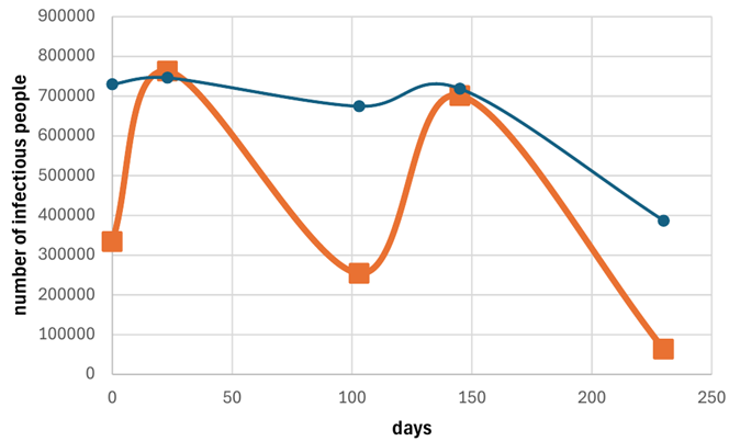
This bimodal function has 2 maximums and one minimum with extremal values \[i_{dmax}(23)\approx746097,\quad i_{dmin}(103)\approx674355,\quad i_{dmax}(145)\approx718631,\] and \(i_{d}(0)\approx729759, i_{d}(230)\approx386677.\)

One may compare these values with the observed extremal values: \[i_{stat}(23)=762754,\quad i_{stat}(103)=253884,\quad i_{stat}(145)=701112.\] and \(i_{stat}(0)=333849,\quad i_{stat}(230)=63298.\)

Note that from the SIR model well-known formula ([4,8]) by taking \(S_0\approx 0.47,k=.97\) one gets a larger maximum value: \[i_{SIRmax}=N(1-k+k\ln(k/S_0))\approx 7431128.\]

So, our SLIR model lacks fit outside of the peak values.

We don’t know if it is possible to get a better fit by using formula (13) in the case of bimodal distribution of spread. Note that the better fit is possible in the case of unimodal distribution.

Conflicts of Interest: The author declares no conflict of interest.

Data Availability: No datasets were generated or analyzed during the current study.

Funding Information: This research did not receive any specific grant from funding agencies in the public, commercial, or not-for-profit sectors.

Appendix

Lemma 4. From conditions \[\tag{79} R_0<2k(k-\sqrt{S_0}),\quad 0<m<\frac{k\sqrt{8}}{\sqrt{(1-\delta^2)[2k(k-\sqrt{S_0})-R_0]}},\] we get \(0<C_1<1,\quad C_2>0,\quad w=C_1x(t)>0\).

Proof. Indeed, from (12) in view of (79) we have \[C_2=\left(R_0+\frac{8k^2}{m^2}-2k^2+2k\sqrt{S_0}\right)(1-\delta^2)+ \frac{8k^2\delta^2}{m^2}>0.\]

Since \(C_2>0\) the expression in (11) \[C_1:=\frac{4k\mp m\sqrt{2C_2}}{4k\pm m\sqrt{2C_2}},\] is real. Further from (11) in the case \(\pm1=1\) we have \(C_1<1\) and \[C_1=\frac{4k-m\sqrt{2C_2}}{4k+m\sqrt{2C_2}} =\frac{16k^2-2m^2C_2}{(4k+m\sqrt{2C_2})^2}.\]

So, we get \(0<C_1<1\) if \[\frac{8k^2}{m^2}-C_2>0,\] or \[\frac{8k^2}{m^2}>C_2=\left(R_0-2k^2+2k\sqrt{S_0}\right)(1-\delta^2)+ \frac{8k^2}{m^2},\] which follows from (79). The same is true in the case \(\pm1=-1\). □

Lemma 5. From conditions (79) and \[\tag{80} t-t_0<-\frac{m}{2q_0}\ln(C_1),\] we get \(0<w<1,\quad I_1(w)>0\).

Proof. From Lemme 3.4 we have \(w=C_1e^{2q_0(t-t_0)/m}>0\) and from condition (80) we get \(w<1.\) □

Lemma 6. From conditions \(x>0,\delta>0\) we get \[\tag{81} 1+\delta+(1-\delta)x^{2m\delta/b}>(1-\delta)(1+x^{2m\delta/b}).\]

Proof. \[1+\delta+(1-\delta)x^{2m\delta/b}-(1-\delta)(1+x^{2m\delta/b})=2\delta>0.\] □

Lemma 7. From conditions \(m>0,C_1>0\) and \[\tag{82} x>\frac{8k}{C_1m^{3/2}(1-\delta)\sqrt{1+\delta}},\quad \hbox{or}\quad t-t_0>\frac{m}{2q_0} \ln\left(\frac{8k}{C_1m^{3/2}(1-\delta)\sqrt{1+\delta}}\right),\] we get \(I_1<1\).

Proof. \[I_1=\frac{64k^2w(1-w)(1+x^{2m\delta})}{m^3(1+w)^3(1-\delta^2)(1+\delta+(1-\delta)x^{m\delta})} <\frac{64k^2w}{m^3(w)^3(1-\delta^2)(1-\delta)}<1,\] if \[C_1x=w^2>\frac{64k^2w}{m^3(w)^2(1-\delta^2)(1-\delta)},\] which follows from (82). □

Lemma 8. From condition \[\tag{83} 0<w<\frac{m+1}{2+\sqrt{m^2+3}},\] we get \(m+1-4w+(1-m)w^2>0\).

Proof. The inequality \[m+1-4w+(1-m)w^2=(1-m)(w-w_1)(w-w_2)>0,\] is true if \(m>1\) and \(w_1<w<w_2\), where \[w_1=\frac{-2-\sqrt{3+m^2}}{m-1}<0,\quad w_2=\frac{-2+\sqrt{3+m^2}}{m-1} =\frac{m+1}{2+\sqrt{m^2+3}}>0,\] and Lemme 8 is followed from condition (83). □

Lemma 9. From conditions (79) and \[\tag{84} t-t_0<\frac{m}{2q_0}\ln\left(\frac{m+1}{C_1(2+\sqrt{m^2+3})}\right),\] we get \(I_1(w)+L_1(w)>0\).

Proof. From Lemma 4 we get \(w>0\) and from (84) we get (83), and from Lemma 8 we get \(m+1-4w+(1-m)w^2>0\), so the statement is followed from the formula (6). □

Lemma 10. By choosing \(\pm 1=1\) in (60) and assuming \[\tag{85} 0<m< \frac{4k^2}{|R_0+2k\sqrt{S_0}-2k^2|(1-\delta^2)},\quad 0<\delta<1,\] we get \[C_5=\frac{2k(1+m)-m\sqrt{2C_4}}{2k(1-m)+ m\sqrt{2C_4}}> 0,\quad w=C_5x>0.\]

Proof. Indeed, \[C_5=\frac{2k(1+m)-m\sqrt{2C_4}}{2k(1-m)+ m\sqrt{2C_4}}=\frac{2k-m(\sqrt{2C_4}-2k)}{2k+m(\sqrt{2C_4}-2k)} =\frac{4k^2-m^2(\sqrt{2C_4}-2k)^2}{(2k+m(\sqrt{2C_4}-2k))^2}> 0,\] if \[4k^2-m^2(\sqrt{2C_4}-2k)^2>0,\] or \[4k^2m^{-2}-(2C_4-4k\sqrt{2C_4}+4k^2)> 0\] \[4k\sqrt{2C_4}> 2C_4+4k^2-4k^2m^{-2}\] \[32k^2C_4>(2C_4+4k^2-4k^2m^{-2})^2,\] and from (59) \[C_4=(R_0+2k\sqrt{S_0})(1-\delta^2)+2k^2(\delta^2+k^2/m^2)>0,\] we get \[32k^2C_4-(2C_4+4k^2-4k^2m^{-2})^2= \frac{64k^4}{m^2}-4(2k\sqrt{S_0}-2k^2+R_0)^2>0.\] □

Lemma 11. By choosing \(\pm 1=1\) in (60) and assuming \[\tag{86} 1\le m< \frac{4k^2}{|R_0+2k\sqrt{S_0}-2k^2|(1-\delta^2)},\quad 0<\delta<1,\] we get \(I_2(t)>0.\)

Proof. The statement is followed from (13) and Lemma 10. □

Lemma 12. From conditions \[\tag{87} w>0,\quad m>\frac{2k}{\sqrt{C_3(1-\delta^2)}},\quad 0.6<\delta<1,\quad \frac4{3-\delta}<m<\frac1{\delta},\] we have \[L_2(w)>0.\]

Remark 10. Note that the condition \(0.6<\delta<1\) in (87) is very restrictive and could be improved. For example, if \(\delta=0.2\) and \(1\le m<2.7\) then the discriminant of \[(m-1)(2m-1)w^2+4(m^2-1)+(m+1)(2m+1)-(1+w)(m+1+m-mw)m(1+\delta)w,\] with respect to w is negative and the conditions \(0.6<\delta<1,\quad \frac1{\delta}<m<\frac4{3-\delta}\) in Lemma 12 may be improved.

Proof. From (13) we have \[I_2(w)=\frac{8k^2w(1+m+w(m-1))(1+x)^{2m\delta})}{m^3(1+w)^3(1-\delta^2)(1+\delta+(1-\delta) (1+x^{2m\delta}))},\] and using inequality (81) we get \[I_2<\frac{8k^2w(1+m+w(m-1))}{m^3(1+w)^3(1-\delta^2)(1-\delta)}.\]

Further from (15) we have \[\begin{aligned} L_2(w)=&C_3 -I_2(w)-\frac{4k^2}{m^2(1-\delta^2)^2} +\frac{8k^2w[(m-1)(2m-1)w^2+4(m^2-1)w+(m+1)(2m+1) ] }{m^4(1+w)^4(1-\delta^2)^2}\\ >&C_3 -\frac{4k^2}{m^2(1-\delta^2)^2}\\ &+\frac{8k^2w[(m-1)(2m-1)w^2+4(m^2-1)w+(m+1)(2m+1) ] }{m^4(1+w)^4(1-\delta^2)^2}- \frac{8k^2w(1+m+w(m-1))}{m^3(1+w)^3(1-\delta^2)(1-\delta)}\\ =&C_3 -\frac{4k^2}{m^2(1-\delta^2)^2} +\frac{8k^2w}{m^4(1+w)^4(1-\delta^2)^2}\\ &\times[(m-1)(2m-1)w^2+4w(m^2-1)+(m+1)(2m+1)-(1+w)(m+1+m-mw)m(1+\delta)]\\ =&C_3 -\frac{4k^2}{m^2(1-\delta^2)^2} +\frac{8k^2w}{m^4(1+w)^4(1-\delta^2)^2}\\ &\times[(m^2(3+\delta)-3m+1)w^2+(3m-m\delta-4)(m+1)w+(2m+1)(1-m\delta)], \end{aligned}\] and the statement is followed from conditions (87) in view of \[C_3>\frac{4k^2}{m^2(1-\delta^2)},\] \[1-m\delta>0,\quad 3m-m\delta-4>0,\] and \[m^2(3+\delta)-3m+1=\left(m\sqrt{3+\delta}-\frac3{\sqrt{3+\delta}}\right)^2+1-\frac{9}{12+4\delta} >0.\] □

Corollary 1. From conditions \[1\le m< \frac{4k^2}{|R_0+2k\sqrt{S_0}-2k^2|(1-\delta^2)},\quad m>\frac{2k}{\sqrt{C_3(1-\delta^2)}},\] \[\tag{88} 0.6<\delta<1,\quad \frac1{\delta}<m<\frac4{3-\delta},\] we have \[S_2(w)>0,\quad I_2(w)>0,\quad L_2(w)>0.\]

Remark 11. In the case \[k=0.97,\quad S_0=0.47, \delta= 0.61,\quad m=1.67,\quad R_0=0.01,\] conditions (88) are satisfied. The positivity of \(S_2\) follows from 14.

For the proof of Lemma 3 see the following page from Wolfram Mathematica (one trivial solution is dropped.): \[\begin{aligned} H_0 :=\;& C_0-a_1p_0^2p_1^2p_2-2a_2p_0^2p_1^2p_2 -a_1p_0^2p_1p_2^2-2a_2p_0^2p_1p_2^2 \\ &+2a_2p_0^2p_1^2p_2^2+2a_1p_0p_1p_2q_0 +a_0q_0^2-a_0q_0^2\delta^2 +\frac{a_0^2q_0^2(-1+\delta^2)}{2k}, \\[6pt] H_1 :=\;& \frac{a_1(a_0-k)q_0^2(\delta^2-1)}{k} +p_0\Bigl( a_1p_0(p_1^2+4p_1p_2+p_2^2) \\ & +2a_2p_0(p_1^2-2p_1^2p_2-2p_1p_2^2+p_2^2+4p_1p_2) +4a_2p_1p_2q_0 -2a_1q_0(p_1+p_2) \Bigr), \\[6pt] H_2 :=\;& \frac{\bigl(a_1^2+2a_2(a_0-k)\bigr)q_0^2(\delta^2-1)}{2k}-p_0\Bigl( 3a_1p_0(p_1+p_2) -2a_2p_0(p_1^2+p_2^2-3p_2-3p_1+4p_1p_2) \\ & -2a_1q_0+4a_2q_0(p_1+p_2) \Bigr), \\[6pt] H_3 :=\;& 2a_1p_0^2+4a_2p_0^2-4a_2p_0^2p_1 -4a_2p_0^2p_2+4a_2p_0q_0 +\frac{a_1a_2q_0^2(-1+\delta^2)}{k}, \\[6pt] H_4 :=\;& 2a_2p_0^2+\frac{a_2^2q_0^2(-1+\delta^2)}{2k}. \end{aligned}\]

\[\operatorname{Simplify}\!\left[ \operatorname{Solve}\!\left( \{H_0=0,H_1=0,H_2=0,H_3=0,H_4=0\}, \{a_0,a_2,a_1,q_0,C_0\} \right) \bigg/\!\left. \{p_2\to p_3+2-p_1\} \right. \right]\]

\[\begin{aligned} \Biggl\{& \left\{ a_2\to0,\quad a_1\to0,\quad C_0\to -\frac{a_0(a_0-2k)q_0^2(-1+\delta^2)}{2k} \right\}, \\[6pt] &\left\{ a_0\to \frac{ k\left(16p_1^2-16p_1(2+p_3)+p_3^2(-1+\delta^2)\right) }{ p_3^2(-1+\delta^2) }, \right.\\ &\hspace{2.5cm} a_2\to-\frac{16k}{p_3^2(-1+\delta^2)}, \quad a_1\to\frac{16k(2+p_3)}{p_3^2(-1+\delta^2)}, \\ &\hspace{2.5cm}\left. q_0\to\frac{p_0p_3}{2}, \quad C_0\to\frac{1}{8}kp_0^2p_3^2(-1+\delta^2) \right\}, \\[6pt] &\left\{ a_0\to \frac{ k\left(4p_1^2-4p_1(2+p_3) +p_3(4+p_3+p_3\delta^2)\right) }{ p_3^2(-1+\delta^2) }, \right.\\ &\hspace{2.5cm} a_2\to-\frac{4k}{p_3^2(-1+\delta^2)}, \quad a_1\to\frac{8k}{p_3^2(-1+\delta^2)}, \quad q_0\to p_0p_3, \\ &\hspace{2.5cm}\left. C_0\to \frac{ kp_0^2\left( -16-16p_1^2-16p_3+16p_1(2+p_3) +p_3^2(-3-2\delta^2+\delta^4) \right) }{ 2(-1+\delta^2) } \right\} \Biggr\}. \end{aligned}\]