
Piles are fundamental components of civil and geotechnical engineering systems because they transfer superstructure loads to deeper soil layers. Their dynamic response to lateral excitations, including seismic, wind, hydrodynamic, and machine-induced actions, is therefore important for structural safety and serviceability [1,2]. Conventional pile models frequently rely on linear structural behavior and simplified soil reactions; such assumptions may become inadequate when deformations are moderate to large or when the surrounding soil exhibits nonlinear response [1]. More generally, nonlinear effects can strongly influence the prediction of deflections, internal forces, and stresses in civil engineering systems, although the magnitude and direction of the resulting deviation from linear predictions depend on loading conditions and the adopted constitutive model. Kenmogne et al. [3,4] investigated nonlinear beams resting on elastic foundations, while related work examined nonlinear oscillations in mechanically coupled sieve systems [5]. These studies reported complex responses including chaotic oscillations, bursting-like vibrations, and regular or irregular impulse patterns associated with nonlinear stiffness, dissipation, and delayed feedback. Such observations emphasize that nonlinear dynamics are not confined to pile–soil systems, but arise in a broad class of structural and mechanical systems whose effective stiffness and energy dissipation depend on response amplitude and excitation conditions.
Nonlinear control is relevant across civil, aerospace, mechanical, and electrical engineering because nonlinear systems may exhibit bifurcation, hysteresis, internal resonance, or chaotic behavior that cannot be inferred reliably from a purely linear description. In civil engineering, nonlinearities may arise from large deformations, material inelasticity, contact and separation, and complex soil–structure interaction; each of these mechanisms can alter the structural response under dynamic loading [6]. Associated effects may include stiffness degradation, amplitude-dependent response, and large strains, thereby motivating the use of nonlinear analytical or numerical models, including finite-element formulations. Appropriate control strategies are consequently important when the objective is to limit vibration and maintain acceptable structural performance, particularly for structures founded on compliant soils or exposed to transient and sustained dynamic actions.
In aerospace applications, nonlinear control techniques such as backstepping, sliding-mode control, and nonlinear formation control are used to manage coupled flight dynamics and preserve stability under changing operating conditions [7]. In robotics, adaptive and nonlinear control approaches are likewise employed to accommodate parameter uncertainty and nonlinear manipulator dynamics, thereby improving trajectory-tracking performance [8]. These examples illustrate the broader role of nonlinear control in engineering systems for which conventional linear controllers may provide only limited validity outside a restricted operating region.
The motivation for this study is the need for models that can represent, within a common analytical setting, the geometric nonlinearity of the pile, nonlinear soil reaction, and modal coupling. Classical analytical approaches remain valuable for physical interpretation but can become restrictive when applied to complex geometries, heterogeneous soils, and nonlinear lateral response [9]. Numerical procedures based on modal reduction, spatial semi-discretization, and Runge–Kutta time integration provide complementary means of examining nonlinear response and assessing control concepts [10]. Accordingly, the present work offers an exploratory application of Lagrangian modeling, a pairwise-coupled three-oscillator approximation, separate nonlinear PDE simulations, and delayed modal PD control to depth-dependent lateral pile loading. These techniques are established in structural dynamics and control; related beam–foundation studies have already combined nonlinear modeling with delayed feedback [3,4]. The present investigation is therefore positioned as an application-level synthesis rather than as a new numerical solver or a fundamentally new control law, and no claim of superiority over the cited methods is made.
The scientific problem addressed in this study concerns the prediction and control of transverse pile displacements under non-uniform harmonic and constant lateral loading while accounting for geometric and soil nonlinearities. Three research questions are considered: (1) How do geometric nonlinearity and nonlinear soil reaction influence the modal dynamics of the idealized pile? (2) To what extent can delayed PD feedback applied in the modal domain attenuate transverse vibration under the stated assumptions? and (3) How can modal reduction and direct numerical treatment of the governing PDE be used as complementary descriptions of responses under prescribed lateral excitation?
The overall objective is to examine an analytical and numerical framework for simulating and controlling the response of an idealized nonlinear pile subjected to lateral excitation. The specific objectives are: (1) to formulate a Lagrangian model incorporating flexural deformation, nonlinear axial stretching, and nonlinear soil reaction; (2) to apply modal projection to reduce the transverse PDE to a finite system of coupled modal equations; and (3) to formulate and assess delayed PD feedback for attenuation of the retained modal responses. The principal assumptions are that: (i) the pile is homogeneous and has uniform linear mass and flexural properties; (ii) the foundation reaction is represented by a nonlinear Winkler-type law; and (iii) energy dissipation is represented by local viscous damping. These assumptions define an idealized analytical model and are not independently validated by the reported numerical examples. In addition, no matched experimental benchmark or systematic modal–PDE convergence study is provided, so the calculations should be interpreted as exploratory rather than predictive.
The remainder of the paper is organized as follows. §2 presents the modeling assumptions, Lagrangian formulation, governing equations, and modal reduction. §3 describes the numerical simulations, including modal calculations and a separate spatial semi-discretization of the nonlinear PDE integrated by a fourth-order Runge–Kutta scheme. §4 develops the delayed PD controller for the retained modes and discusses the associated linearized stability conditions. Finally, §5 summarizes the main findings, limitations, and perspectives for future investigation.
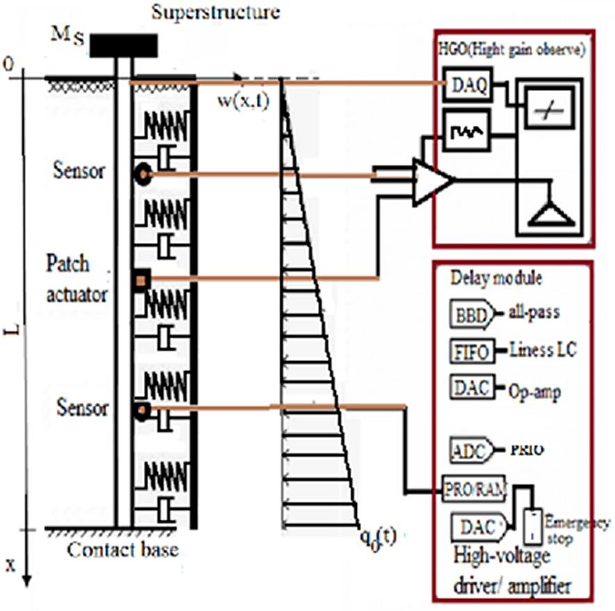
The study considers a single pile of length \(L\), as illustrated in Figure 1. The pile axis is described by the coordinate \(x\), with the head located at \(x=0\) and the tip at \(x=L\). The pile head may be connected to a superstructure or platform. To obtain a tractable planar model, the transverse displacement \(w(x,t)\) is assumed to occur in a single lateral direction.
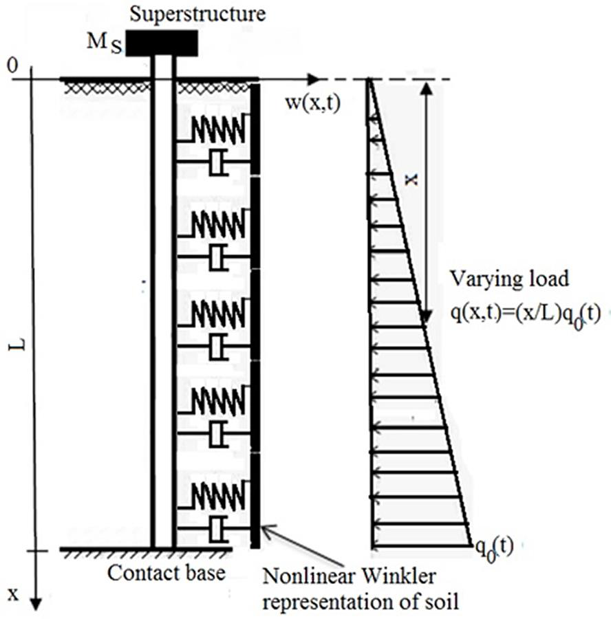
The pile is characterized by the mass per unit length \(m=\rho A\), the area moment of inertia \(I\), and the bending stiffness \(EI\). Interaction between the pile and the surrounding soil is represented by a distributed reactive foundation law. Nonlinear Winkler and \(p\)–\(y\) formulations are widely used for idealized lateral pile response [11,12], while related continuum-to-Winkler representations provide additional background on lateral soil–foundation interaction [13]. The adopted soil reaction may be written as:
or, more generally, as a nonlinear constitutive law \(p_s(w,x)=F(w,x)\). An additional axial load \(P_0(t)\), either compressive or tensile, could interact with the lateral displacement and modify the global stability characteristics. Such a load is not included in the equations or simulations reported below; hence, \(P_0=0\) throughout the present calculations. The time dependence of \(q(x,t)\) represents prescribed external forcing rather than parametric excitation. Geometric nonlinearity is introduced through the axial extension associated with moderate transverse rotations. The corresponding approximate axial strain is \(\varepsilon_{ax}\approx \frac{1}{2}(\partial_x w)^2\). Under the axial-restraint assumption adopted here, the induced axial force \(N(w)\) is nonlocal and depends on the integral of the squared displacement gradient. A standard reduced expression consistent with nonlinear beam mechanics is [14]:
Eq. (2) requires axial end restraint, zero net change in the end separation, and negligible axial inertia; it therefore does not describe an axially free cantilever. The lateral boundary conditions introduced below are independent of this axial-restraint assumption. The Euler–Bernoulli representation further assumes a slender, linearly elastic pile and neglects shear deformation and rotary inertia. Finally, distributed viscous damping is represented by a local coefficient \(c(x)\), which provides an idealized description of energy dissipation in the pile–soil system.
This subsection presents the Lagrangian formulation adopted for the pile–soil–superstructure idealization and derives the nonlinear governing equation from the kinetic energy, potential energies, external work, and dissipation terms. The formulation is consistent with established dynamic pile modeling approaches and soil–pile interaction representations [15,16].
The pile is modeled as an Euler–Bernoulli beam of length \(L\), flexural rigidity \(EI\), and linear mass density \(\rho A\). A lumped mass \(M_s\), representing the superstructure, may be attached at the pile head \(x=0\) and assigned the lateral displacement \(W_s(t)\). The surrounding soil exerts the nonlinear distributed reaction \(p_s(w,x)\) [11,17]. For a rigid lateral connection between the pile head and the superstructure, \(W_s(t)=w(0,t)\). However, the fixed-head idealizations used in the simulations impose \(W_s=0\); consequently, the head mass and the generalized head force \(Q_s\) do not contribute to the simulated lateral response. Dynamic motion of the superstructure itself is therefore outside the scope of the reported calculations.
The total kinetic energy includes the contributions of the distributed pile mass and the lumped head mass:
where \(w(x,t)\) denotes the lateral displacement field along the pile and the overdot denotes differentiation with respect to time [14].
The bending strain energy of the Euler–Bernoulli pile is:
which represents the classical Euler–Bernoulli flexural response [18].
The soil reaction is represented by a nonlinear distributed foundation potential. For the polynomial law adopted in the illustrative calculations, the corresponding potential energy is:
More generally, one may write \(V_f=\int_0^L V_s(w,x)\,dx\), with \(\partial V_s/\partial w=p_s(w,x)\), where \(p_s(w,x)\) denotes the nonlinear soil reaction [16]. The cubic law used here is an idealized reversible approximation; no calibrated \(p\)–\(y\) curve, interface-separation law, or cyclic degradation model is supplied.
The restrained axial stretching induced by lateral displacement contributes the additional potential energy:
The prescribed distributed lateral load \(q(x,t)\) and the generalized head force \(Q_s(t)\) perform the external work:
where \(q(x,t)\) denotes the prescribed lateral loading. Dynamic lateral pile loading and experimentally observed soil–pile response are discussed, for example, in the field study of Dezi et al. [19].
Distributed viscous damping is introduced through the Rayleigh dissipation function:
where \(c(x)\geq0\) is the local viscous damping coefficient [20]. Eq. (8) contains only linear distributed viscous damping; no nonlinear or concentrated head-damping term is included.
The Lagrangian functional is then written as:
Applying the Euler–Lagrange principle, with \(\dot{w}=w_t\), together with the functional derivatives of the external work and Rayleigh dissipation, gives the governing equation in variational form:
Here, \(\delta L/\delta w\) contains the variations associated with bending, the foundation potential, and nonlocal axial stretching. In the beam interior, \(\delta W_{ext}/\delta w=q(x,t)\), whereas the concentrated head force contributes through the boundary work.
The corresponding strong form of the governing PDE obtained from Eq. (10) is:
For the cubic soil law in Eqs. (1) and (5), and for spatially uniform \(m\), \(EI\), \(c\), \(k_1\), and \(k_3\), Eq. (11) reduces to:
where
Boundary conditions.
For the clamped-head case, \(M_{\mathrm{head}}\) and \(Q_{\mathrm{head}}\) are reaction quantities rather than additional prescribed boundary conditions. A moving or elastically restrained head would require a separate connection law and force balance, neither of which is simulated in the present study.
Initial conditions.
To determine the linear reference modes, the cubic term \(k_3w^3\) and the geometric nonlinearity \(\gamma w_{xx}=\left(\frac{EA}{2L}\int_0^L(w_x)^2dx\right)w_{xx}\) are neglected, and the prescribed lateral excitation \(q(x,t)\) is set to zero. For weak damping, the undamped spatial problem is solved first and damping is introduced subsequently in the modal equations [18,20,21]. The corresponding linearized reference equation is:
Setting \(c=0\) in Eq. (16) and assuming separable solutions \(w(x,t)=\phi(x)\,T(t)\), \(T(t)=e^{i\omega t}\), we obtain the spatial eigenvalue problem:
Seeking spatial solutions of the form \(\phi\propto e^{rx}\) gives the characteristic equation:
The corresponding eigenfunctions \(\phi(x)\) depend on the selected boundary conditions, for example cantilever, simply supported, or clamped–clamped conditions. For a cantilever:
with characteristic equation \(\cosh(\beta L)\cos(\beta L)=-1\). The first roots satisfy \(\beta_1L\approx1.8751\) and \(\beta_2L\approx4.6941\). For simply supported ends, \(\beta_nL=n\pi\) and \(\phi_n(x)=\sin(n\pi x/L)\).
A complete set of orthogonal eigenfunctions \(\{\phi_n(x)\}_{n\geq1}\) satisfying the selected linear boundary conditions is used as the spatial basis. These functions satisfy:
The lateral displacement is expanded as:
where \(q_n(t)\) are the generalized modal coordinates, \(\varphi_n=\phi_n\), and \(m_n=M_n\). Substitution into the governing PDE followed by Galerkin projection gives the modal coefficients:
The geometric nonlinear coefficient becomes:
The resulting \(N\)-mode equations can therefore be written as:
where the generalized modal forces are:
Eqs. (22)–(25) are used below with the simply supported basis and without a moving head mass. For a nonlinear clamped–free modal reduction, the effective-shear boundary contribution must also be included; merely inserting linear cantilever modes into this strong-form projection is not sufficient to obtain a consistent nonlinear clamped–free reduction.
◆ Single-mode case (\(N=1\)). If \(w(x,t)=q(t)\varphi(x)\), \(\int_0^L\varphi^2(x)\,dx=1\), and \([\varphi\varphi’]_0^L=0\), as for the simply supported basis adopted below, then \(\gamma(t)=\frac{EA}{2L}Aq^2\), where \(A=\int_0^L(\varphi'(x))^2dx\) and \(D=\int_0^L\varphi^4(x)\,dx\). The reduced equation is
Eq. (26) has the form of a forced Duffing oscillator, a classical nonlinear system that has been studied extensively in the literature [20]. Because the purpose of the present work is to retain modal interaction, this single-mode limit is not examined further.
◆ Three-mode case (\(N=3\)). Consider the normalized sinusoidal basis \(\varphi_n(x)=\sqrt{\frac{2}{L}}\sin(n\kappa x)\), with \(\kappa=\pi/L\). Direct integration over \(0\leq x\leq L\) gives:
The cubic projection coefficients include the diagonal terms \(T_{nnnn}=3/(2L)\) for \(n=1,2,3\) and the pairwise terms \(T_{nnmm}=1/L\) for \(n\ne m\). However, coefficients such as \(T_{1113}=-1/(2L)\) and \(T_{1223}=1/(2L)\), together with their permutations, are also nonzero. Eq. (29) omits the corresponding mixed cubic terms and should therefore be interpreted as a pairwise-coupled three-oscillator approximation rather than the exact three-mode Galerkin truncation of Eq. (24). Because no averaging or asymptotic smallness argument is introduced to eliminate these terms, this approximation constitutes a modeling limitation. For the linearly varying load \(q(x,t)=q_0(t)x\), the retained modal forces are:
Here, \(q_0(t)\) denotes a load gradient. The schematic in Figure 1, by contrast, labels the tip intensity by \(q_0(t)\) when \(q=(x/L)q_0(t)\); that tip intensity is equal to \(L\) times the gradient used in Eq. (28). These two conventions therefore require an explicit factor-of-\(L\) conversion. Defining \(\zeta=c/m\), \(\omega_n^2=(k_1+EIn^4\kappa^4)/m\), \(\alpha_1=3k_3/(2mL)\), \(\alpha_2=EA\pi^4/(2mL^5)\), and \(F_0(t)=F(t)=(S/m)q_0(t)\), the pairwise-coupled three-mode approximation becomes:
For \(F_0(t)=0\), the system in Eq. (29) always admits the trivial equilibrium \((0,0,0)\). Algebraic candidates with all three components nonzero may be written as \((\pm q_{10},\pm q_{20},\pm q_{30})\), where
These expressions follow by introducing the first-order variables \(q_{ip}=\dot q_i\), setting all time derivatives to zero, and assuming \(\alpha_1(5\alpha_1-98\alpha_2)\ne0\). Eight real nonzero candidates exist only if all three right-hand sides of Eq. (30) are positive; equilibrium branches containing one or more zero components, as well as singular parameter combinations, require separate treatment. For the positive values of \(\alpha_1\), \(\alpha_2\), and \(\omega_i^2\) used in the simulations, each restoring bracket in the unforced version of Eq. (29) is positive, so the origin is the only real unforced equilibrium. A nonzero constant force shifts the equilibrium, whereas harmonic forcing precludes a time-independent forced equilibrium. To examine local stability of an admissible unforced equilibrium, the perturbation \(q_i(t)=q_{i0}+Q_i e^{st}\) is introduced, where \(Q_i\) is infinitesimal and \(s\) is the complex growth rate [22]. Linearization then yields
with
Eq. (31) admits a nontrivial perturbation vector if and only if the following characteristic equation is satisfied:
At the trivial equilibrium \((0,0,0)\), Eq. (33) factorizes into three modal quadratic factors, with roots \(s_{i\pm}=\frac{1}{2}\left(-\zeta\pm i\sqrt{4\omega_i^2-\zeta^2}\right)\). When \(\zeta=0\) and \(\omega_i^2>0\), the linearized unforced modes are neutrally oscillatory; this local property does not imply that every nonlinear multimode trajectory is periodic. When \(\zeta>0\) and \(\zeta^2<4\omega_i^2\), each linearized mode is a damped stable focus.
The pairwise-coupled system in Eq. (29) was examined numerically under two prescribed excitation scenarios: harmonic time-varying forcing and constant forcing. Unless otherwise stated, the simulations used the following nondimensional or normalized oscillator parameters:
The frequencies in Eq. (34) are prescribed oscillator parameters rather than values generated from the spectrum \(\omega_n^2=(k_1+EIn^4\kappa^4)/m\): no single set of constant \(k_1\), \(EI\), \(m\), and \(L\) produces the stated nonzero \(1{:}2{:}3\) frequency ratios. With the adopted spatial normalization, \(q_n\) carries units of length\(^{3/2}\), while \(\zeta=c/m\) has dimensions of inverse time and is therefore a damping coefficient rather than a conventional dimensionless damping ratio. A physical calibration linking these modal parameters to a specific pile geometry and soil profile is not provided.
The reported figures are interpreted using the parameter values stated in the manuscript. However, the value of \(S/m\), the modal initial conditions, time-integration settings, transient-exclusion rule, and any spectral normalization are not reported, which limits quantitative reproducibility. In addition, the modal and PDE calculations use different boundary idealizations and parameterizations and should therefore be regarded as separate numerical illustrations rather than a matched-model validation. In the discussion below, the terms “bursting-like” and “noisy-like” refer only to the appearance of the finite-time waveforms; no slow–fast classification, stochastic forcing model, Lyapunov exponent, or other chaos diagnostic is used to assign a dynamical regime.
For the time-varying case, the prescribed load gradient is \(q_0(t)=A_0\cos(\omega t)\) with \(A_0=5\times10^{-2}\).
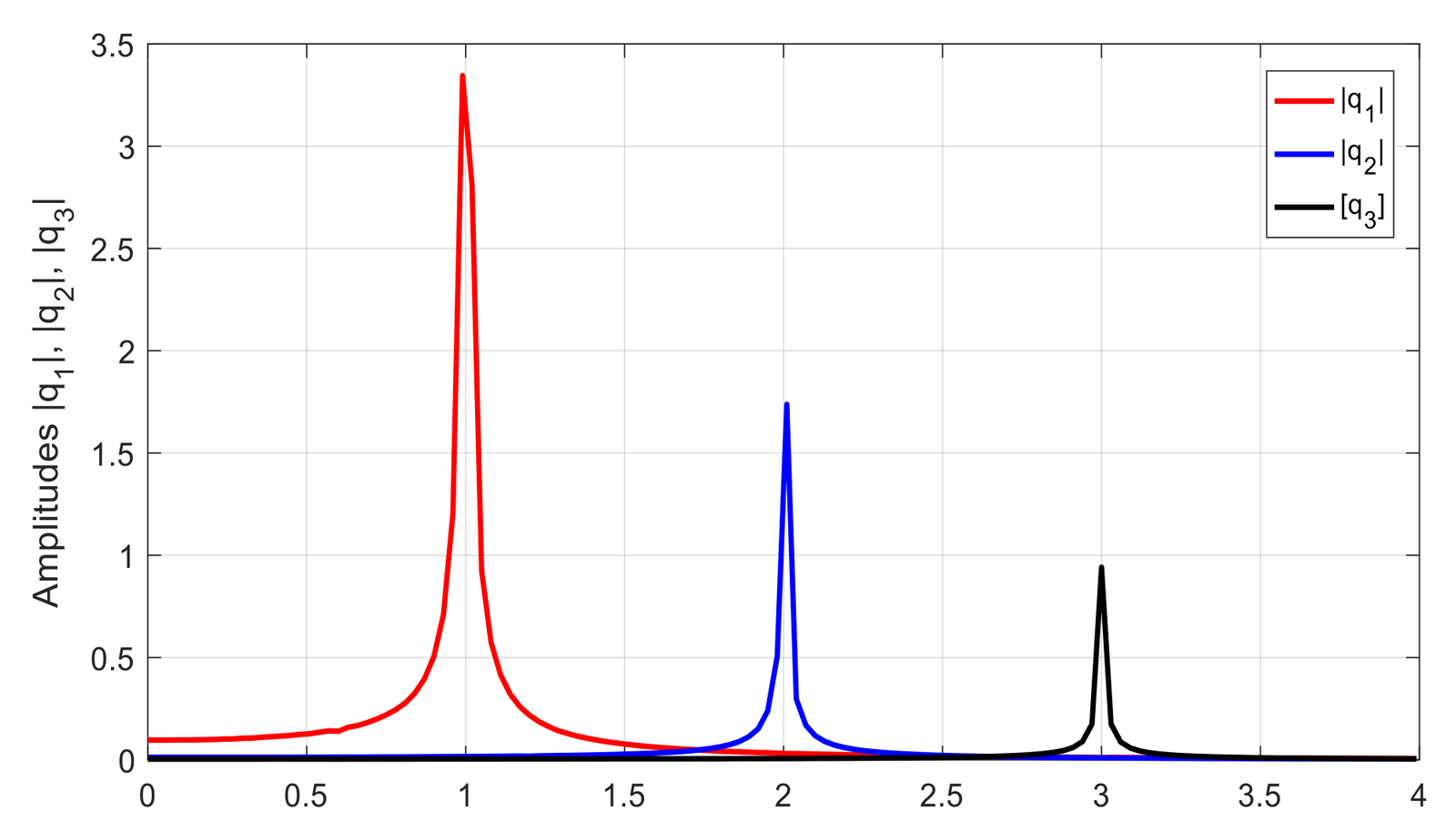
Figure 2 presents the maximum modal amplitudes reported for the parameter set in Eq. (34). Each generalized coordinate \(q_i\) exhibits a peak in the vicinity of its prescribed modal frequency \(\omega_i\). Because the frequency-sweep increment, integration duration, transient-removal procedure, and amplitude-extraction window are not specified, these curves are best interpreted qualitatively rather than as a reproducible frequency-response function.
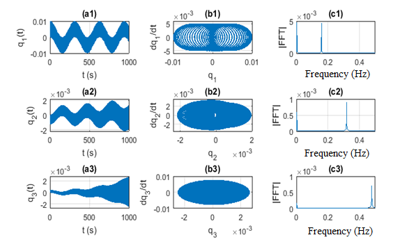
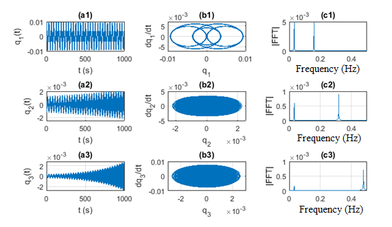
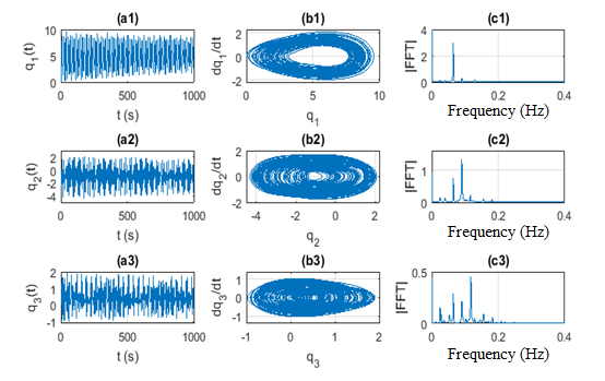
Figures 3–7 illustrate representative modal responses for several excitation frequencies. At \(\omega=0.2\) (Figure 3), mode 1 exhibits a comparatively regular bursting-like pattern, mode 2 shows intermittent amplitude packets, and mode 3 displays a sequence of pulse-like envelopes. At the lower excitation frequency \(\omega=0.02\) (Figure 4), modes 1 and 3 retain bursting-like features, whereas mode 2 appears more irregular over the plotted interval. At \(\omega=1.7\) (Figure 5), the traces exhibit amplitude modulation on a noticeably different time and amplitude scale. These descriptions refer to finite-time waveform morphology and do not, by themselves, establish bifurcation, chaos, or stochastic dynamics.
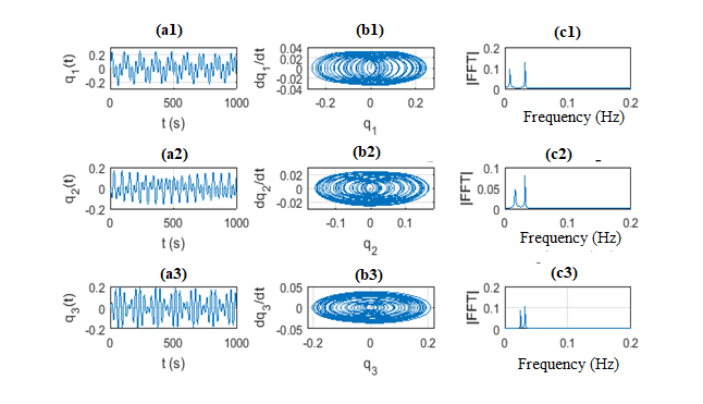
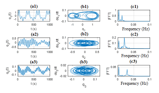
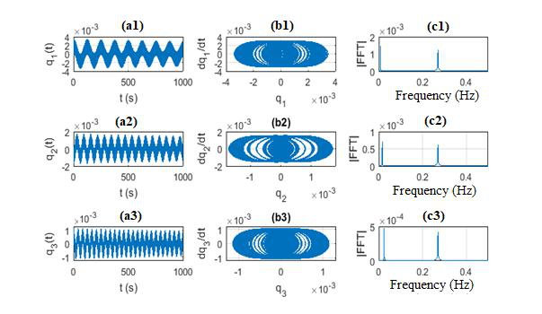
Comparison of Figures 3–5 shows that, although all three cases use the same prescribed relation \(\omega_1=\omega_2/2=\omega_3/3=5\times10^{-2}\), the finite-time response changes appreciably with excitation frequency. The low-frequency case \(\omega=0.02\) contains a more irregular mode-2 waveform, the intermediate case \(\omega=0.2\) contains more organized amplitude packets, and the higher-frequency case \(\omega=1.7\) exhibits a different modulation pattern. Because no scalar complexity measure, bifurcation diagram, or spectral criterion is reported for this sweep, the comparison should not be interpreted as a quantified monotonic change in dynamical complexity.
When the prescribed modal relation is changed to \(\omega_1=\omega_2/2=\omega_3/3=1\), the responses in Figures 6 and 7 differ from those obtained with the lower modal frequencies. Mode 1 remains bounded over the displayed interval and develops repeated amplitude packets, whereas modes 2 and 3 remain smaller but show gradual changes in amplitude. Figures 3 and 7 share the same reported excitation frequency but use different prescribed natural frequencies; the same is true of Figures 4 and 6. These paired comparisons demonstrate sensitivity to the prescribed modal frequencies, but they do not constitute an asymptotic stability analysis or a quantitative measurement of intermodal energy transfer.
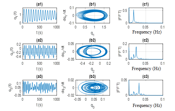
For constant excitation, the prescribed load gradient is \(q_0(t)=A_0\). Figures 8 and 9 compare two forcing amplitudes while maintaining \(\omega_1=\omega_2/2=\omega_3/3=5\times10^{-2}\). For \(A_0=5\times10^{-2}\) (Figure 8), mode 1 shows a damped oscillatory transient, while modes 2 and 3 exhibit amplitude-packet or bursting-like behavior over the plotted interval. Increasing the load amplitude by one order of magnitude to \(A_0=5\times10^{-1}\) (Figure 9) produces larger and more irregular finite-time oscillations. This waveform irregularity does not establish chaos. Under constant forcing, the symmetric restoring terms in Eq. (29) admit a mechanical potential that includes the constant-load work, and for \(\zeta>0\) the mechanical energy decreases at the rate \(-\zeta\sum_i\dot q_i^2\). Consequently, a sustained nonstationary chaotic attractor is not consistent with this autonomous dissipative formulation. The irregular response in Figure 9 should therefore be interpreted as a transient response, or potentially as a consequence of numerical settings that cannot be assessed from the reported information, rather than as evidence of a transition to sustained chaos.
To examine the distributed nonlinear response directly, we return to Eq. (12) and introduce the following nondimensional variables:
where \(L\) is the pile length, \(W_0\) is a characteristic transverse displacement, and \(T=1/\omega_0\) is the bending time scale associated with the Euler–Bernoulli operator. The resulting dimensionless coefficients and forcing function are defined by:
The nondimensional governing equation is therefore:
Here, \(I(\tau)\) denotes the dimensionless slope integral \(I(u(\cdot,\tau))\) and should not be confused with the dimensional area moment of inertia \(I\) used in the beam stiffness. The spatial and temporal domains are \(\xi\in(0,1)\) and \(\tau>0\). For a prescribed lateral load that increases linearly with depth, the dimensionless excitation is taken as:
Eq. (37) is treated by the method of lines: the spatial derivatives are approximated by finite differences and the resulting system of ordinary differential equations is integrated in time using a fourth-order Runge–Kutta method. For convenience, the dimensionless curvature variable \(M=u_{\xi\xi}\) is introduced.
For the clamped–free boundary-value problem, the head conditions are \(u(0,\tau)=0\) and \(u_\xi(0,\tau)=0\). At the free lateral tip, the bending-moment condition is \(M(1,\tau)=u_{\xi\xi}(1,\tau)=0\), while the effective-shear condition is \(M_\xi(1,\tau)-\mu I(u)u_\xi(1,\tau)=0\). The latter follows from the same stretching energy and is not, in general, equivalent to imposing only \(u_{\xi\xi\xi}=0\). The retained numerical figures do not document the endpoint closure that was actually used; consequently, this aspect of the implementation cannot be independently reproduced from the manuscript alone.
The spatial grid is defined by \(\xi_i=ih\), \(h=1/N_x\), and \(i=0,\ldots,N_x\). Ghost points may be introduced to impose the derivative boundary conditions, including \(u_{-1}\) for the clamped-slope condition at \(\xi=0\) and an endpoint extension near \(\xi=1\) for the moment and effective-shear conditions. At interior nodes, the centered approximations are
The centered interior differences in Eq. (39) are second-order accurate in space. A consistent Runge–Kutta implementation must enforce the complete boundary conditions and reevaluate both the forcing and the nonlocal quantity \(I(u)\) at every Runge–Kutta stage. The grid size, time step, endpoint stencils, numerical stability restrictions, and spatial or temporal refinement tests used to generate the retained plots are not reported. Accordingly, the numerical results are interpreted as qualitative illustrations and not as a documented convergence study.
For time integration, define the auxiliary velocity variable \(v=u_\tau\). The semi-discrete formulation is based on the following first-order-in-time system:
The initial conditions are \(u(\xi,0)=u_0(\xi)\) and \(v(\xi,0)=0\). The nonlocal functional \(I(u)\) may be approximated numerically by the composite trapezoidal rule:
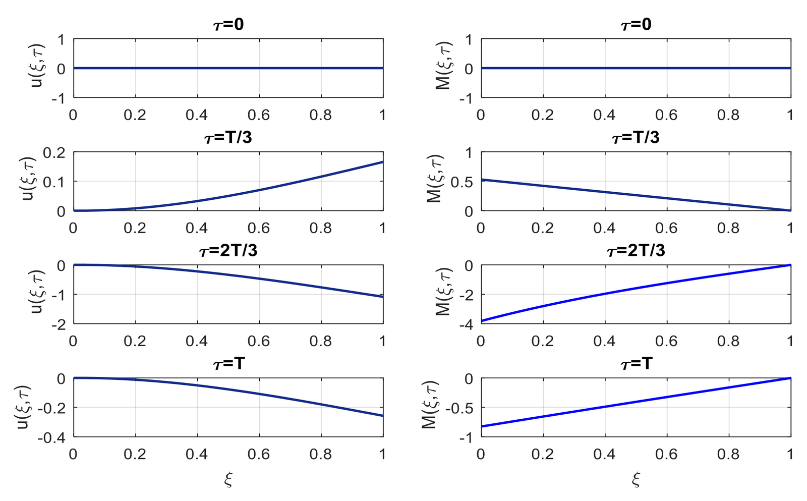
The PDE calculations use the representative dimensionless parameters \(\delta=0.05\), \(\mu=1\), and \(A_0=1\), while \(\alpha\), \(\beta\), and the excitation frequency are varied between cases. The prescribed forcing is \(f(\xi,\tau)=A_0\xi\cos(\Omega\tau)\), and the initial displacement is taken as \(u_0(\xi)=0\). This formulation retains both the nonlocal stretching contribution through \(I(u)\) and the cubic foundation term. The selected values are illustrative dimensionless parameters rather than a calibration to a specific pile, soil profile, or field test. In Figures 10–16, the caption symbol \(\omega\) denotes the dimensionless excitation frequency \(\Omega=\omega_{\mathrm{dim}}T\), while \(A_0\) denotes the dimensionless amplitude of \(Q\) and is distinct from the modal load-gradient amplitude used in §3. The variable \(M\) is dimensionless curvature; the corresponding dimensional bending-moment scale is \(EIW_0/L^2\). Image labels written as \(\xi=L/2\) and \(\xi=2L/3\) should be interpreted as the physical locations \(x=L/2\) and \(x=2L/3\), equivalently \(\xi=1/2\) and \(2/3\). The snapshot label \(T\) appearing in Figures 11 and 16 is not defined independently of the reference time scale and therefore cannot be interpreted quantitatively without the original plotting convention.
Case of time-varying excitation (\(\omega\neq0\))
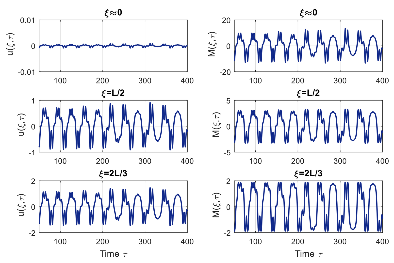
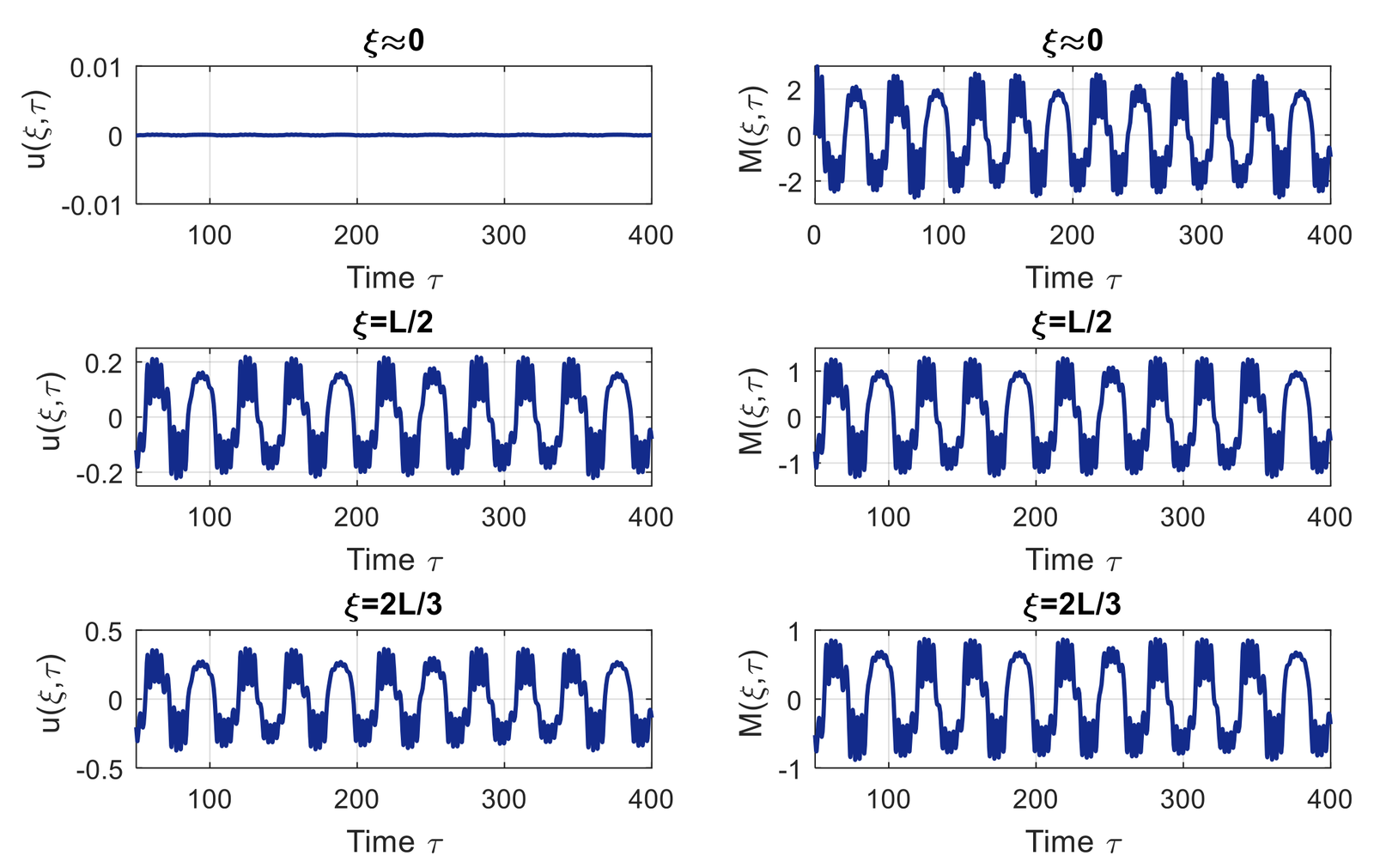
Figure 10 shows the temporal evolution of displacement and curvature-related moment for \(\alpha=0.25\), \(\beta=0.125\), and \(\omega=0.2\). The calculated response is amplitude modulated and is qualitatively reminiscent of the finite-time waveform in Figure 4; however, the two simulations use different boundary conditions, coefficients, and scalings, so this similarity cannot be treated as a modal–PDE validation. Figure 11 presents the corresponding spatial profiles at selected instants. The displayed profiles describe the spatial distribution of the computed state but do not determine a propagation velocity or demonstrate negligible wave propagation. They may be compared qualitatively with dynamic pile studies such as [23,24], although no matched geometry, constitutive model, or loading case is available for a quantitative benchmark.
Figure 12, obtained for \(\alpha=0.05\), \(\beta=5.125\), and \(\omega=1\), exhibits a different modulation pattern and response scale. Because \(\alpha\), \(\beta\), and the excitation frequency all differ from the values used for Figure 10, the comparison does not isolate the effect of any single parameter, including the cubic foundation coefficient \(\beta\). The response may be placed in the broader context of nonlinear foundation dynamics [25,26], but the cited studies do not constitute matched benchmarks for the present dimensionless calculation.
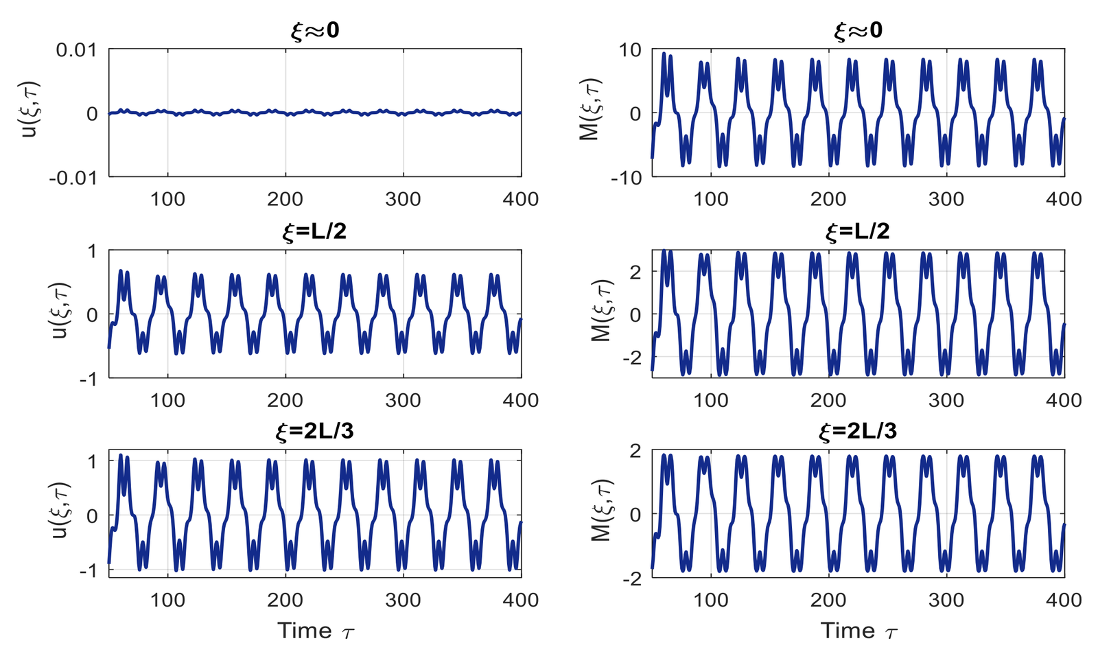
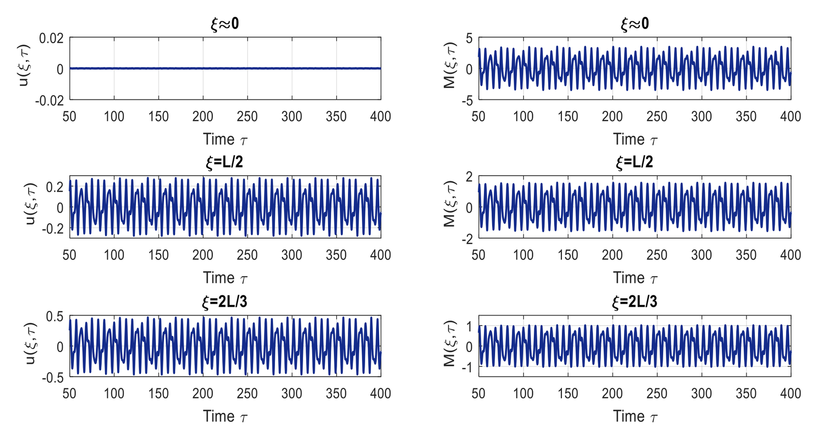
Figures 13 and 14 provide a more direct comparison because they retain \(\alpha=0.02\) and \(\omega=0.2\) while changing \(\beta\) from \(0.125\) to \(5.125\). This is a 41-fold increase in the cubic foundation coefficient and therefore represents a substantial, rather than incremental, parameter change. The traces display different finite-time modulation patterns and amplitudes, but neither spectral bandwidth nor a localization index is evaluated. The results can be compared qualitatively with nonlinear beam–soil interaction analyses [26] and with numerical or experimental pile-dynamics studies [23,27]; they should not be interpreted as a quantitative validation of those studies.
Case of constant excitation (\(\omega=0\))
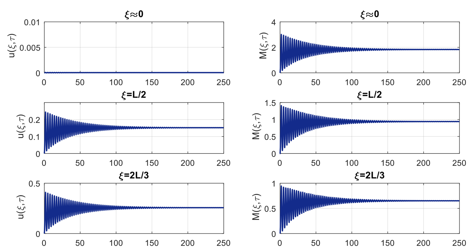
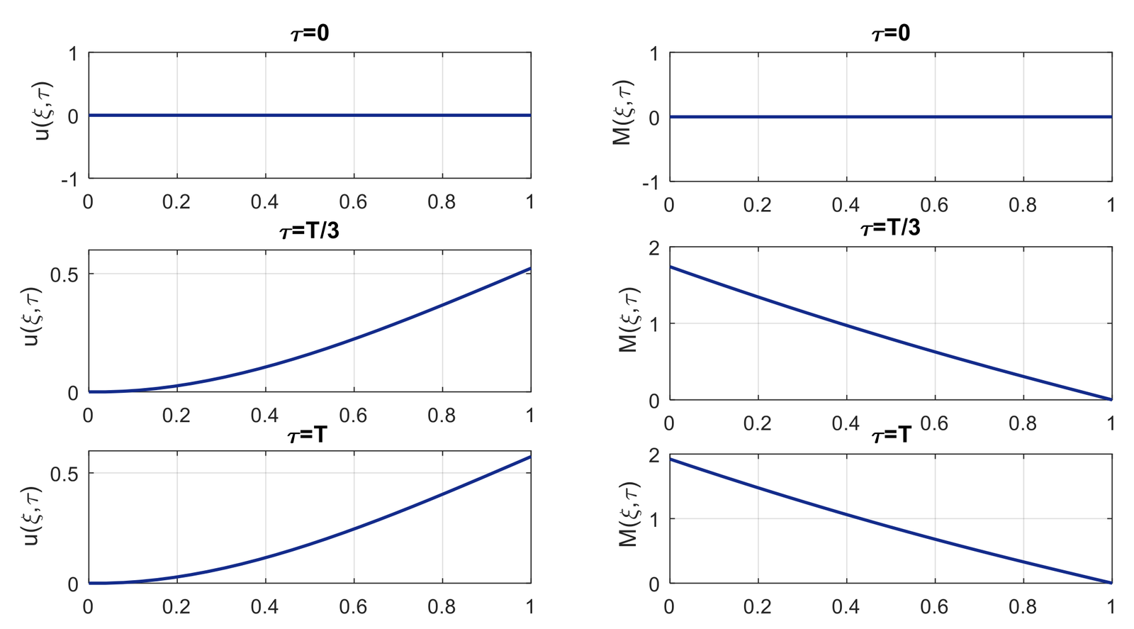
Figure 15 illustrates the temporal evolution of the displacement and curvature-related moment under constant excitation. Over the displayed interval, the response approaches a steady level, as expected for a damped autonomous system subjected to a constant load. Figure 16 shows the corresponding spatial evolution: the plotted displacement vanishes at the clamped end \(\xi=0\) and reaches its largest displayed value near \(\xi=1\), whereas the bending response is greatest near the clamped end and approaches zero at the free tip. These trends are consistent with the stated finite-length clamped–free lateral idealization, but they do not represent a semi-infinite soil medium and do not independently verify the unreported numerical implementation of the effective-shear boundary condition.
The trends in Figures 10–16 may be compared qualitatively with established theoretical work on nonlinear pile or beam–foundation dynamics [25,26]. Nevertheless, the present manuscript does not provide a common geometry, constitutive parameter set, loading history, or error metric for a quantitative comparison. Likewise, the calculations are not directly validated against field or experimentally anchored pile studies such as [19,27]. This distinction is important because visual agreement in waveform shape or deformation pattern is not equivalent to validation of the governing model or numerical implementation.
We now reconsider the retained temporal dynamics in modal form. Let \(q_i(t)\) denote the generalized coordinate of mode \(i=1,2,3\). A delayed proportional–derivative (PD) controller is applied independently to each retained mode, following the general framework of time-delay feedback control [28]. Eq. (42) is based on the pairwise approximation in Eq. (29); ideal modal-state measurement and independent modal actuation are therefore assumed.
With
The delayed control input applied to each modal equation is defined by:
In dimensional time, \(k_{p,i}\) has units of inverse time squared, \(k_{d,i}\) has units of inverse time, and \(u_i\) is a mass-normalized generalized control force. The delay \(\tau\) used in this section is measured in the time units of \(t\) and is distinct from the dimensionless time coordinate introduced in §3.3. Linearization about the unforced origin, where the derivatives of the cubic restoring terms vanish, gives the delayed second-order modal equation [28,29]:
At the distributed beam/pile level, a formal feedback term can be expressed as:
Here, \(g_{act}(x)\) represents both the actuator’s spatial distribution and the dimensional conversion required for \(u_c\) to have the same units as the distributed load \(q(x,t)\). Because neither the actuator/sensor projection nor a specific form of \(g_{act}(x)\) is supplied, Eq. (46) and the arrangement in Figure 17 are conceptual rather than a demonstrated physical implementation of independent modal feedback. Possible spillover into unmodeled modes, measurement noise, actuator saturation, finite bandwidth, and uncertainty in the time delay are not evaluated.
For the unforced linearized equation, assume a modal perturbation of the form \(q_i(t)\propto e^{st}\). The resulting characteristic equation is transcendental because of the delay term [28,29]. For compactness, the mode index is suppressed below, so \(\omega=\omega_i\) denotes a natural frequency rather than the external excitation frequency:
At an imaginary-axis stability crossing, set \(s=j\Omega\) and separate the real and imaginary parts of the characteristic equation, as commonly done in frequency-domain analyses of delayed feedback systems [28,29]:
The corresponding real and imaginary equations are:
For each positive crossing frequency \(\Omega\) satisfying \((\Omega^2-\omega^2)^2+\zeta^2\Omega^2=k_p^2+k_d^2\Omega^2\), the corresponding candidate delays are
Here, \(\operatorname{atan2}(y,x)\) selects the appropriate phase quadrant. A valid delay margin additionally requires stability at zero delay, enumeration of all positive crossing frequencies, and identification of the first crossing that causes loss of stability. Consequently, Eq. (50) provides candidate delays and does not, by itself, constitute a nonlinear or global stability guarantee.
For sufficiently small delay, the first-order expansion \(e^{-s\tau}\approx1-s\tau\) may be introduced. Substitution into Eq. (47) gives
For a positive leading coefficient, Routh–Hurwitz stability of this truncated quadratic requires:
The third condition requires \(k_p>-\omega^2\), while the first two yield the screening bounds
These inequalities constitute only a small-delay screening rule for the truncated quadratic and are meaningful when \(|s\tau|\ll1\) for the roots of interest. They do not constrain every root of the exact transcendental characteristic equation and therefore cannot certify robust tuning or nonlinear stability of the original controlled system.
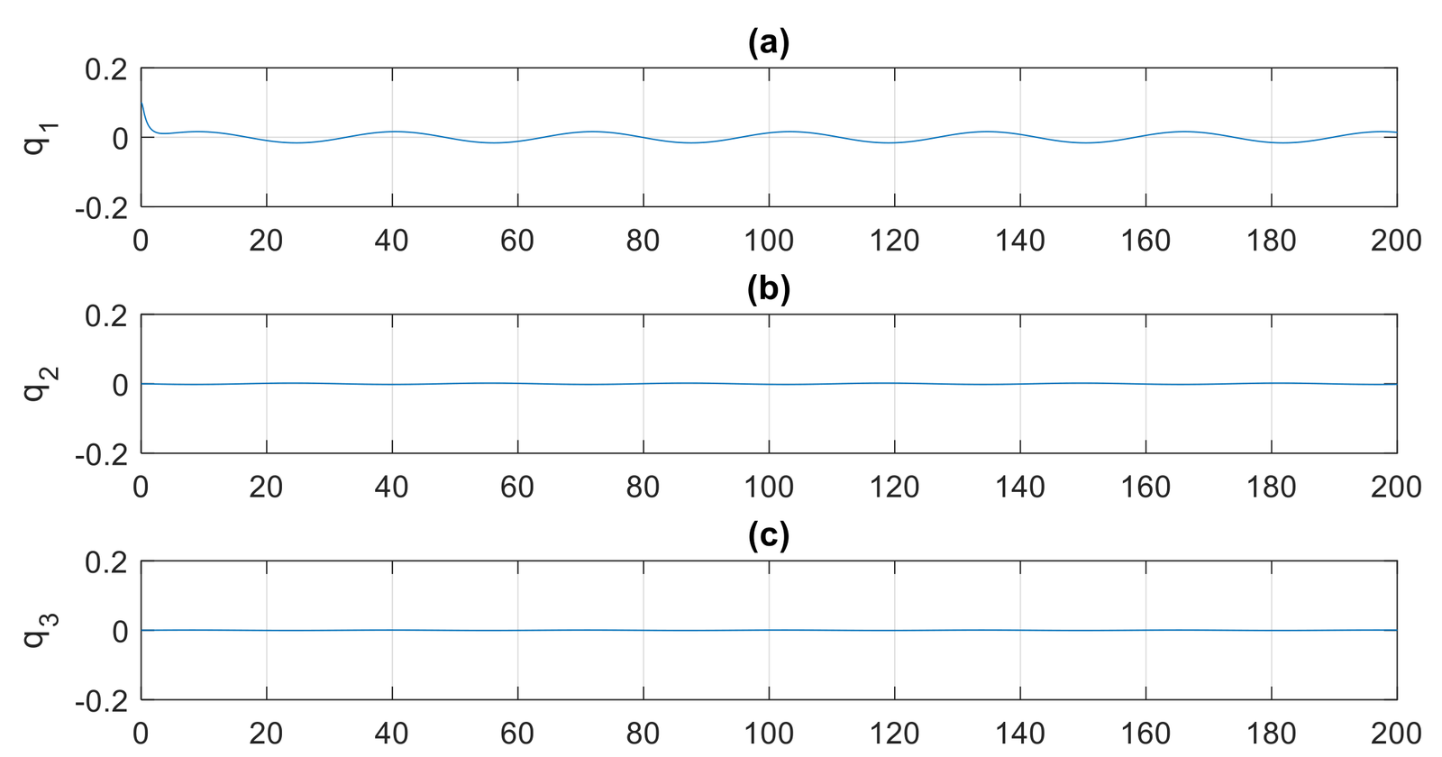
The reported controlled simulation uses Eq. (42) together with the delayed controller in Eq. (44), with \(k_p=[3;\ 12;\ 27]\), \(k_d=[4;\ 8;\ 12]\), and \(\tau=0.1\). The retained source description is inconsistent concerning the uncontrolled baseline: the surrounding text points to Figure 3, whereas the original caption points to Figure 4; because those figures use different excitation frequencies, a strictly matched before-and-after comparison cannot be reconstructed. The controlled response shown in Figure 18 retains a mode-1 oscillation. Under persistent nonzero forcing, the origin is not itself a solution of Eq. (42), so delayed PD feedback should be interpreted as vibration attenuation rather than as a mechanism that necessarily enforces exact zero displacement.
For mode 3, \(1-k_{d,3}\tau=1-12(0.1)=-0.2\), so the stated gains do not satisfy the first small-delay screening condition in Eq. (52). Failure of this approximate condition does not prove instability of the exact delay differential equation; determining stability for all retained modes requires an exact characteristic-root computation or a complete crossing analysis. Such a numerical delay-margin calculation is not reported. Moreover, the history functions on \([-\tau,0]\), interpolation of delayed states, integration step, controller activation protocol, and actuator effort are unspecified. Figure 18 therefore demonstrates a controlled response under one reported parameter set but does not establish robustness, optimality, energetic efficiency, or a quantified improvement relative to a consistently matched uncontrolled baseline.
This study examined an analytical and numerical framework for the nonlinear dynamic response and delayed feedback control of piles subjected to prescribed lateral excitation. The Lagrangian formulation incorporates geometric nonlinearity, nonlinear Winkler-type soil reaction, and modal coupling under the stated axial-restraint assumption. Two complementary numerical descriptions were considered: a pairwise-coupled three-oscillator approximation based on simply supported sinusoidal modes and a separate clamped–free PDE calculation. Because these descriptions employ different boundary idealizations and parameter conventions, they should be regarded as distinct numerical investigations rather than as a validated unified simulation of a single soil–pile–superstructure system.
The reported modal and PDE plots exhibit approximately periodic, dissipative, amplitude-modulated, bursting-like, mixed, and irregular finite-time responses. The waveform patterns vary as the excitation frequency, forcing amplitude, and dimensionless foundation coefficients are changed. Nevertheless, no systematic bifurcation analysis, Lyapunov-exponent calculation, spectral-complexity metric, or slow–fast classification is reported, so the simulations do not establish a formal sequence of dynamical regimes or a monotonic increase in complexity. Under constant modal excitation, the larger-load response is irregular over the displayed interval; because the underlying constant-force system is autonomous and dissipative, the figure should be interpreted as a transient response rather than as evidence of a sustained chaotic attractor.
The relative modal amplitudes and phases demonstrate sensitivity to modal coupling, although energy exchange among modes is not quantified explicitly. In the PDE calculations, the plotted spatial distributions are consistent with the stated clamped–free lateral idealization: the largest displayed bending response occurs near the pile head, whereas the largest displacement occurs near the tip. These qualitative features are physically interpretable, but the manuscript does not provide a matched analytical solution, experimental benchmark, convergence study, or fully documented endpoint stencil with which to verify the numerical boundary closure quantitatively.
A delayed proportional–derivative controller was also examined in the modal domain as a means of attenuating the retained vibration coordinates. The analytical treatment identifies candidate imaginary-axis crossings and derives a first-order small-delay screening rule for the unforced linearized modes. These results do not determine optimal gains and do not constitute a proof of global nonlinear stability. The controlled trace retains forced oscillations, while the absence of a consistently matched uncontrolled baseline and complete delay-integration details prevents a reliable quantitative estimate of attenuation. Robustness to parameter uncertainty, actuator limitations, unmodeled modes, and delay variation therefore remains an open issue.
Overall, the contribution is an exploratory application of established nonlinear beam modeling and delayed PD control to prescribed depth-dependent lateral pile loading. The value of the study lies in bringing the Lagrangian formulation, modal coupling, direct PDE calculations, and delayed feedback discussion into a common application context rather than in introducing a fundamentally new numerical algorithm or controller. Before the framework can be used predictively in engineering design, physical calibration, complete numerical specifications, systematic verification of the retained simulations, and matched validation against field or laboratory data are required. In particular, the present forcing functions are idealized; seismic, hydrodynamic, wind-specific, and machine-induced loading cases have not been validated within the proposed framework.
Beyond the verification needs identified above, several research perspectives are envisioned:
Future investigations should extend the model to pile groups and stratified or heterogeneous soils, for which pile–pile interaction, layering, and spatial stiffness variation can substantially modify the overall dynamic response.
Extending the formulation to coupled axial, lateral, and torsional motion would provide a more complete representation of pile foundations subjected to multidirectional dynamic loading.
Future work may also examine whether vibration energy can be recovered or exploited in semi-active damping concepts. Such developments would require explicit transducer, actuator, and energy-balance models before claims regarding sustainable or energy-efficient foundation systems can be assessed.
Author Contributions: All authors contributed equally to the conception, development, and preparation of the manuscript. All authors have read and approved the final version of the manuscript for publication.
Conflicts of Interest: The authors declare that there are no conflicts of interest related to this work.
Data Availability: No datasets were generated or analyzed during the present study; therefore, data availability is not applicable.
Funding Information: This research received no external funding.
The components below describe a conceptual arrangement, not an experimental setup. The numerical hardware ranges are illustrative, not selected or tested specifications. Here \(f_c\) is the filter cutoff, \(f_s\) the sampling frequency, and \(f_{\max}\) the highest frequency to be retained.