
Interconnection networks are very important in computer networking and useful for the transformation between the computer and processor. In last few years, many researchers designed the new interconnection networks. In parallel processsing system, interconnection networks plays an important role to increase the performance of computers. In graph theory, interconnection network can be expressed by a graph. In this expression, processor represented by vertex and connection between the units represented by an edge. From the topology of a network, we can easily determine certain properties. The number of links (edges) connected to a node known as the degree of that node (vertex). If the degree is same for all nodes in a network, then network is called regular network [1]. The degree of a vertex is represented by \(\{d_{v}|v\in V\left(\aleph\right)\}\) of a graph \(\aleph.\) The sum of the neighborhood degree of a vertex \(v\in \aleph\) is the sum of degrees of all adjacent vertices of a vertex \(v\) and it is denoted by \(S_v.\)
In graph theory and the characterization of the structural characteristics of graphs and networks, graph invariants are crucial. The chemical structure of molecules, the internet, chemical reactions, computers, and social networks are all described in this. Topological indices are these indices that we employ to investigate the abstract structural features of networks. There are three types of topological indices: degree-based [2], distance-based [3,4], and spectrum-based topological indices [4,6].
The first degree-based topological index was put forward in \(1975\) by Milan Randić, [7]. It is define as \[\label{Aj1} R_{\alpha}\left(\aleph\right)=\sum_{uv\in E\left(\aleph\right)}\left(d_u d_v\right)^{\alpha}, ~~~\alpha=-1,-\frac{1}{2},\frac{1}{2},1.\tag{1}\] Later, this index was generalized for any real number \(\alpha,\) and known as the generalized Randić index, [8] and its mathematical expression is \[\label{Aj2} RR_{\alpha}\left(\aleph\right)=\sum_{uv\in E\left(\aleph\right)}\frac{1}{\left(d_u d_v\right)^{\alpha}}.\tag{2}\] Gutman and Trinajstic, introduced the first Zagreb index in [9], mathematically can be written as \[M_{1}\left(\aleph\right)=\sum_{v\in E\left(\aleph\right)}d_v^2=\sum_{uv\in E\left(\aleph\right)}\left(d_u+d_v\right).\tag{3}\] The general sum-connectivity index [10], defined as \[SCI\left(\aleph\right)=\sum_{uv\in E\left(\aleph\right)}\frac{1}{\sqrt{d_u+d_v}}.\tag{4}\] Vukicevic et al. [11], introduced the geometric arithmetic index and expressed as \[\label{Aj3} GA\left(\aleph\right)=\sum_{uv\in E\left(\aleph\right)}\frac{2\sqrt{d_ud_v}}{d_u+d_v}.\tag{5}\] The \(5^{th}\) geometric arithmetic index was introduced by Graovac et al. [12], its formulation is \[\label{Aj4} GA_5\left(\aleph\right)=\sum_{uv\in E\left(\aleph\right)}\frac{2\sqrt{S_uS_v}}{S_u+S_v}.\tag{6}\] There are many other types of degree based topological indices like, general Randić index, general sum connectivity index, second Zagreb index, third Zagreb index, first multiple Zagreb index, second multiple Zagreb index, hyper Zagreb index, augmented Zagreb index, harmonic index, reduced second Zagreb index, reduced reciprocal Randić index, modified Zagreb index, symmetric division index and inverse sum index, briefly defined in [13].
The M-polynomial was introduced by Deutsch and Klavzar [14] in 2015. It functions similarly to the Hosoya polynomial [15] in determining the closed form of numerous degree-based topological indices. For more detail on the recent study of topological indices and their applications see [16-24]. This motivates us to study M-polynomial of some graph operations and some interconnection networks. Recently, the study of M-polynomial are reported in [25-33].
The M-polynomial can be defines as \[\begin{aligned} M\left(\aleph;x,y\right)=\sum_{ i\leq j}m_{i,j}\left(\aleph\right)x^{i}y^{j}, \end{aligned}\tag{7}\] where \(m_{i,j}\left(\aleph\right)\) is the number of edges of graph \(\aleph\) such that \(i\leq j.\)
| Topological index | Derivation from M(\(\Gamma\);x,y) |
|---|---|
| First Zagreb | \(\left(D_{x}+D_{y}\right)\left(M\left(\aleph;x,y\right)\right)\) |
| Second Zagreb | \(\left(D_{x}D_{y}\right)\left(M\left(\aleph;x,y\right)\right)\) |
| Second modified Zagreb | \(\left(S_{x}S_{y}\right)\left(M\left(\aleph;x,y\right)\right)\) |
| General Randić | \(\left(D_{x}^{\alpha}D_{y}^{\alpha}\right)\left(M\left(\aleph;x,y\right)\right)\) |
| General inverse Randić | \(\left(S_{x}^{\alpha}S_{y}^{\alpha}\right)\left(M\left(\aleph;x,y\right)\right)\) |
| Symmetric division index | \(\left(D_{x}S_{y}+D_{y}S_{x}\right)\left(M\left(\aleph;x,y\right)\right)\) |
| Harmonic index | \(2S_{x}J \left(M\left(\aleph;x,y\right)\right)\) |
| Inverse sum index | \(S_{x}JD_{x}D_{y}\left(M\left(\aleph;x,y\right)\right)\) |
| Augmented Zagreb | \(S_{x}^{3}Q_{-2}JD_{x}^{3}D_{y}^{3}\left(M\left(\aleph;x,y\right)\right)\) |
where \[\begin{aligned} \label{Aj55} D_{x}&=x\frac{\partial f}{\partial x}, \hspace{1.5cm}S_{x}=\int_{0}^{x}\frac{f\left(z,y\right)}{z}dz, \hspace{1.5cm}Q_{a}=x^{a}f\left(x,y\right), \nonumber \\D_{y}&=x\frac{\partial f}{\partial y}, \hspace{1.5cm}S_{y}=\int_{0}^{y}\frac{f\left(x,z\right)}{z}dz \hspace{1.5cm}~~~ J=f\left(x,x\right). \end{aligned}\tag{8}\]
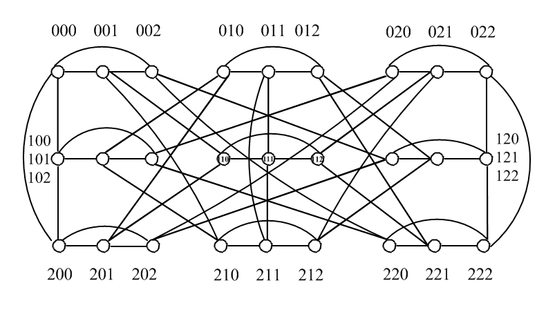
Wenjun et al. [34] introduced a new family of communication architectures called “biswapped networks.” Given any \(n\)-node basis network \(\aleph\), the associated biswapped network \(Bsw(\aleph)\) is built of \(2n\) copies of \(\aleph.\)
We generalize this biswapped network to K-swapped networks for \(t\)-regular graphs. For a base graph \(\aleph\), the K-swapped interconnection networks \(\left(Ksw\left(\aleph_{t}\right)\right)\) are graphs with vertex set and edge set defined as:
The size and degree of K-swapped networks are \(\frac{(t+K-1)Kn^{2}}{2}\) and \((t+K-1)\) respectively, where \(t\) is the regularity of the base graph.
In this section, we study some topological properties of K-swapped networks of \(t\)-regular graphs.
Theorem 1: Let \(\Gamma\) be the K-swapped network of \(t\)-regular graphs, then Randić, general, and reduced reciprocal Randić indices are:
Proof: The K-swapped network has degree \(d=t+K-1\) and size \(\frac{dKn^{2}}{2}\). Substituting these parameters into the formulas, we get:
Theorem 2: Let \(\Gamma\) be the K-swapped network of \(t\)-regular graphs, then the family of Zagreb indices are:
Proof: Using the degree \(d=t+K-1\) and size \(\frac{dKn^2}{2}\) of the K-swapped network, the indices are derived as follows:
Theorem 3: Let \(\Gamma\) be the K-swapped network of \(t\)-regular graphs, then the sum connectivity and general sum connectivity indices are:
Proof: Using the degree and size of the K-swapped network:
Theorem 4: Let \(\Gamma\) be the K-swapped network of \(t\)-regular graphs, then the geometric arithmetic, \(5^{th}\) geometric arithmetic, symmetric division, and inverse sum indices are:
Proof: Using the degree \(d = t + K – 1\) and size \(\frac{dKn^2}{2}\), we derive the indices as follows:
Theorem 5: Let \(\Gamma\) be the K-swapped network of \(t\)-regular graphs, then the M-polynomial is:
\[M(\Gamma; x, y) = \frac{dKn^2}{2}x^d y^d.\]
Proof: The M-polynomial for a graph is given by:
where, \(m_{ij}\left(\Gamma\right)=|E\left(\Gamma\right)|\) and \(i,~j\) are the degree of adjacent vertices \(u,~v\) respectively.
\(M\left(\Gamma;x,y\right)=\frac{Kn^{2}}{2}\left(t+K-1\right)x^{t+K-1}y^{t+K-1}\) and already computed parameter \(d=t+K-1\) then we have \(M(\Gamma;x,y)=\frac{dKn^2}{2}x^dy^d.\)
This completed the proof of M-polynomials for different K-swapped networks derived from \(t\)-regular graphs.
Following theorem is about the subdivided M-polynomials for different topological indices like, family of Zagreb indices and some from Randi\'{c} index.Theorem 6: Let \(\Gamma\) be the K-swapped network of \(t\)-regular graphs, then the M-polynomials for various indices are:
Proof: Consider K-swapped networks of \(t\)-regular graphs. Using “Equation (8)”, we compute different differential formulas with the same \(d = K + t – 1\):
Based on these formulas, we derive the following M-polynomials:
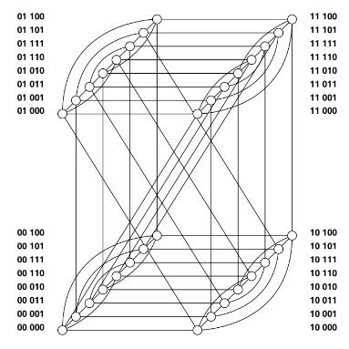
The \(n\)-dimensional twisted cube [35], is a variant of \(n\)-dimensional hypercube cube. It is represented by \(TQ_{n}\) with \(n=2k+1.\) The size, order and degree of \(n\)-dimensional twisted cube are \(n2^{n-1}\) , \(2^{n}\) and \(n\) respectively. To make a twisted cube, we delete some edges from the graph and add some edges in such a way that total number of edges conserved.
Suppose that \(n\) is an odd integer with condition \(n\geq 3.\) We can divide vertices of \(TQ_{n}\) into four sets \(L^{0,0},\) \(L^{0,1},\) \(L^{1,0},\) \(L^{1,1}\) where \(L^{i,j}\) consists of those vertices \(u\) with \(u_{n-1}=i,\) \(u_{n-2}=j\) and \(\left(i,j\right)\in \{\left(0,0\right),\left(0,1\right),\left(1,0\right),\left(1,1\right)\}\) and edge set of twisted cube we can define as: vertex \(u_{n-1}u_{n-2}u_{n-3},\dots,u_{1}u_{0}\) with \(P_{n-3}\left(u\right)=0\) is connected to \(\bar{u}_{n-1} \bar{u}_{n-2} u_{n-3}u_{n-4}…u_{1}u_{0}\) and \(\bar{u}_{n-1} {u}_{n-2} u_{n-3}u_{n-4}…u_{1}u_{0}\); \({u}_{n-1} \bar{u}_{n-2} u_{n-3}u_{n-4}…u_{1}u_{0}\) and \(\bar{u}_{n-1} {u}_{n-2} u_{n-3}u_{n-4}…u_{1}u_{0}\) if \(P_{n-3}\left(u\right)=1.\)
Figure: 2 is drawn for a clearer view of the vertex set of \(5\)-dimensional twisted cube.
This section is about topological indices and M-polynomials of \(n\)-dimensional twisted cube.
Theorem 7. Let \(\chi\) be the \(n\)-dimensional twisted cube network, then Randić, general and reduced reciprocal Randić indices are
1: \(R_{\alpha}\left(\chi\right)=2^{n-1}n^{2\alpha+1}.\)
2: \(RR_{\alpha}\left(\chi\right)=2^{n-1}\left(n\right)^{1-2\alpha}.\)
3: \(RRR\left(\chi\right)=2^{n-1}n\left(n-1\right).\)
Proof. As we know that \(n\)-dimensional twisted cube network has degree \(n\) and size is \(n2^{n-1},\) after plugging all the known parameters in to the formulas
1 \(R_{\alpha}\left(\chi\right) =\sum_{uv\in E\left(\chi\right)}\left(d_u d_v\right)^{\alpha}=n2^{n-1}\left(n\times n\right)^{\alpha}=2^{n-1}n^{2\alpha+1}.\)
2 \(RR_{\alpha}\left(\chi\right) =\sum_{uv\in E\left(\chi\right)}\frac{1}{\left(d_u d_v\right)^{\alpha}}= n2^{n-1}\frac{1}{\left(n\times n\right)^{\alpha}}=2^{n-1}n^{1-2\alpha}. \)
3 \(RRR\left(\chi\right)=\sum_{uv\in E\left(\chi\right)}\sqrt{\left(d_u-1\right)\left(d_v-1\right)}=n2^{n-1}\sqrt{\left(n-1\right)\left(n-1\right)}=n2^{n-1}\sqrt{\left(n-1\right)^{2}} =n2^{n-1}\left(n-1\right).\)
Theorem 8. Let \(\chi\) be the \(n\)-dimensional twisted cube network, then we have family of Zagreb index are
\[ \begin{aligned} &1:\ M_{1}(\chi) = 2^{n}n^{2}.\\ &2:\ M_{2}(\chi) = 2^{n-1}n^{3}.\\ &3:\ M_{3}(\chi) = 0.\\ &4:\ PM_{1}(\chi) = (2n)^{2^{n-1}n}.\\ &5:\ PM_{2}(\chi) = n^{2^{n}n}.\\ &6:\ AZI(\chi) = 2^{n-1}n\left(\frac{n^{2}}{n^{2}-2}\right)^{3}.\\ &7:\ RM_{2}(\chi) = 2^{n-1}n(n-1)^{2}.\\ &8:\ ~^mM_{2}(\chi) = \frac{2^{n-1}}{n}.\\ &9:\ HM(\chi) = 2^{n+1}n^{3}. \end{aligned} \]Proof. As we know that \(n\)-dimensional twisted cube network has degree \(n\) and size is \(n2^{n-1},\) then following indices can be proven by putting parameters into formulas,
\[ \begin{aligned} &1:\ M_{1}(\chi) &= \sum_{uv \in E(\chi)}(d_u + d_v) = n2^{n-1}(n + n) = n2^{n-1}(2n) = 2^{n-1}(2n^2) = 2^{n}n^2.\\ &2:\ M_{2}(\chi) &= \sum_{uv \in E(\chi)}(d_u d_v) = n2^{n-1}(n \times n) = 2^{n-1}n^3.\\ &3:\ M_{3}(\chi) &= \sum_{uv \in E(\chi)}(d_u – d_v) = n2^{n-1}(n – n) = 0.\\ &4:\ PM_{1}(\chi) &= \prod_{uv \in E(\chi)}(d_u + d_v) = (n + n)^{2^{n-1}n} = (2n)^{2^{n-1}n}.\\ &5:\ PM_{2}(\chi) &= \prod_{uv \in E(\chi)}(d_u d_v) = (n^2)^{2^{n-1}n} = n^{2^{n}n}.\\ &6:\ AZI(\chi) &= \sum_{uv \in E(\chi)}\left(\frac{d_u d_v}{d_u d_v – 2}\right)^3 = n2^{n-1}\left(\frac{n^2}{n^2 – 2}\right)^3.\\ &7:\ RM_2(\chi) &= \sum_{uv \in E(\chi)}(d_u – 1)(d_v – 1) = n2^{n-1}(n – 1)(n – 1) = 2^{n-1}n(n – 1)^2.\\ &8:\ ^mM_2(\chi) &= \sum_{uv \in E(\chi)}\frac{1}{d_u d_v} = \frac{n2^{n-1}}{n \times n} = \frac{2^{n-1}}{n}.\\ &9:\ HM(\chi) &= \sum_{uv \in E(\chi)}(d_u + d_v)^2 = n2^{n-1}(n + n)^2 = 2^{n+1}n^3. \end{aligned} \]Theorem 9. Let \(\chi\) be the \(n\)-dimensional twisted cube network, then sum connectivity and general sum connectivity indices are
\[ \begin{aligned} &1:\ SCI(\chi) &= 2^{n-\frac{3}{2}}\sqrt{n}.\\ &2:\ \chi_{\alpha}(\chi) &= 2^{n-1+\alpha}n^{\alpha+1}. \end{aligned} \]Proof: As we know that \( n \)-dimensional twisted cube network has degree \( n \) and size \( n2^{n-1} \), the following indices can be computed in the same manner:
\[ \begin{aligned} &1:\ SCI(\chi) &= \sum_{uv \in E(\chi)}\frac{1}{\sqrt{d_u + d_v}} = \frac{n2^{n-1}}{\sqrt{2n}} = 2^{n-\frac{3}{2}}\sqrt{n}.\\ &2:\ \chi_{\alpha}(\chi) &= \sum_{uv \in E(\chi)}(d_u + d_v)^{\alpha} = n2^{n-1}(2n)^{\alpha} = 2^{n-1+\alpha}n^{\alpha+1}. \end{aligned} \]
Theorem 10. Let \(\chi\) be the \(n\)-dimensional twisted cube network, then the geometric arithmetic, symmetric division and inverse sum index are
\[ \begin{aligned} &1:\ GA(\chi) &= 2^{n-1}n.\\ &2:\ GA_5(\chi) &= 2^{n-1}n.\\ &3:\ SDI(\chi) &= 2^{n}n.\\ &4:\ IS(\chi) &= 2^{n-2}n^{2}. \end{aligned} \]
Proof: The \( n \)-dimensional twisted cube network has degree \( n \) and size \( n2^{n-1} \), thus:
\[ \begin{aligned} &1:\ GA(\chi) &= \sum_{uv \in E(\chi)}\frac{2\sqrt{d_u d_v}}{d_u + d_v} = n2^{n-1}\frac{2\sqrt{n^2}}{2n} = 2^{n-1}n.\\ &2:\ GA_5(\chi) &= n2^{n-1}\frac{2\sqrt{n^2}}{2n} = 2^{n-1}n.\\ &3:\ SDI(\chi) &= \sum_{uv \in E(\chi)}\frac{d_u^2 + d_v^2}{d_u d_v} = n2^{n-1}\frac{n^2 + n^2}{n^2} = n2^{n-1}\frac{2n^2}{n^2} = 2^{n}n.\\ &4:\ IS(\chi) &= \sum_{uv \in E(\chi)}\frac{d_u d_v}{d_u + d_v} = n2^{n-1}\frac{n^2}{2n} = 2^{n-2}n^2. \end{aligned} \]
Theorem 11. : Let \(\chi\) be the \(n\)-dimensional twisted cube network, then M-polynomial is
M(\(\chi\);x,y)=\(n2^{n-1}x^ny^n.\)
Proof. As we know that from the definition of M-polynomials \(M\left(\chi;x,y\right)=h\left(x,y\right)=\sum_{i\leq j}m_{ij}\left(\chi\right)x^{i}y^{j},\) and \(m_{ij}\left(\chi\right)=|E\left(\chi\right)|=2^{n-1}n\) where i,j are the degrees of adjacent vertices \((u,v),\) both have same degree \(n.\) Hence this prove that, \[\begin{aligned} \label{Twisted2} M\left(\chi;x,y\right)=n2^{n-1}x^ny^n. \end{aligned}\] ◻
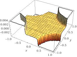
Figure: 3 shows the graphical interpretation of equation (14), that is M-polynomial Table:1 of different twisted cube networks.
Theorem 12. : Let \(\chi\) be the \(n\)-dimensional twisted cube network, then different M-polynomials are:
\[ \begin{aligned} &1:\ M_{1}(\chi;x,y) &= 2^{n}n^{2}(xy)^{n}.\\ &2:\ M_{2}(\chi;x,y) &= 2^{2n-2}n^{4}(xy)^{2n}.\\ &3:\ ^mM(\chi;x,y) &= 2^{2n-2}(xy)^{2n}.\\ &4:\ R_{\alpha}(\chi;x,y) &= 2^{2\alpha(n-1)}n^{4\alpha}(xy)^{2\alpha n}.\\ &5:\ RR_{\alpha}(\chi;x,y) &= 2^{2\alpha(n-1)}(xy)^{2\alpha n}.\\ &6:\ SDI(\chi;x,y) &= 2^{2n}n^{2}(xy)^{2n}.\\ &7:\ H(\chi;x,y) &= 2^{2n-1}n x^{3n}y^{n}.\\ &8:\ IS(\chi;x,y) &= 2^{4n-4}n^{5}y^{3n}x^{5n}.\\ &9:\ AZI(\chi;x,y) &= n^{14}2^{11n-12}x^{12n-2}y^{10n}. \end{aligned} \]Proof. To get M-polynomials of different indices computed by \(“n”\)-dimensional twisted cube, here are some computed formulas necessary for the definition of M-polynomial \[\begin{aligned} D_{x}&=D_{y}=\left(xy\right)^{n}2^{n-1}n^{2},~~~~J=n2^{n-1}x^{2n}.\nonumber\\ S_{x}&=S_{y}=2^{n-1}\left(xy\right)^{n},~~~~Q_{-2}=n2^{n-1}x^{n-2}y^{n}.\nonumber \end{aligned}\] putting all these junctions into definition of M-polynomials, following are different required M-polynomials for different indices,
\[ \begin{aligned} &1:\ M_1(\chi;x,y) &= \left(D_x + D_y\right) M(\chi;x,y) = \left(xy\right)^n 2^{n-1}n^2 + \left(xy\right)^n 2^{n-1}n^2 \\ &&&= 2^n n^2 \left(xy\right)^n. \\ &2:\ M_2(\chi;x,y) &= \left(D_x D_y\right)M(\chi;x,y) = \left(\left(xy\right)^n 2^{n-1}n^2\right) \left(\left(xy\right)^n 2^{n-1}n^2\right) \\ &&&= 2^{2n-2}n^4 \left(xy\right)^{2n}. \\ &3:\ ^mM(\chi;x,y) &= \left(S_x S_y\right)M(\chi;x,y) = \left(2^{n-1}\left(xy\right)^n\right)\left(2^{n-1}\left(xy\right)^n\right) \\ &&&= 2^{2n-2}\left(xy\right)^{2n}. \\ &4:\ R_{\alpha}(\chi;x,y) &= \left(D_x^\alpha D_y^\alpha\right)M(\chi;x,y) = \left(\left(xy\right)^n 2^{n-1}n^2\right)^\alpha \left(\left(xy\right)^n 2^{n-1}n^2\right)^\alpha \\ &&&= 2^{2\alpha(n-1)}n^{4\alpha}\left(xy\right)^{2\alpha n}. \\ &5:\ RR_{\alpha}(\chi;x,y) &= \left(S_x^\alpha S_y^\alpha\right)M(\chi;x,y) = \left(2^{n-1}\left(xy\right)^n\right)^\alpha \left(2^{n-1}\left(xy\right)^n\right)^\alpha \\ &&&= 2^{2\alpha(n-1)}\left(xy\right)^{2\alpha n}. \\ &6:\ SDI(\chi;x,y) &= \left(D_x S_y + D_y S_x\right)M(\chi;x,y) = \left(\left(xy\right)^n 2^{n-1}n^2\right)\left(2^{n-1}\left(xy\right)^n\right) \\ &&&\quad + \left(\left(xy\right)^n 2^{n-1}n^2\right)\left(2^{n-1}\left(xy\right)^n\right) \\ &&&= 2^{2n}n^2\left(xy\right)^{2n}. \\ &7:\ H(\chi;x,y) &= 2S_x JM(\chi;x,y) = 2 \times 2^{n-1}\left(xy\right)^n n2^{n-1}x^{2n} \\ &&&= 2^{2n-1}nx^{3n}y^n. \\ &8:\ IS(\chi;x,y) &= S_x JD_x D_y M(\chi;x,y) = 2^{n-1}\left(xy\right)^n\left(xy\right)^n 2^{n-1}n^2\left(xy\right)^n 2^{n-1}n^2 n2^{n-1}x^{2n} \\ &&&= 2^{4n-4}n^5 y^{3n}x^{5n}. \\ &9:\ AZI(\chi;x,y) &= S_x^3 Q_{-2} JD_x^3 D_y^3 M(\chi;x,y) \\ &&&= \left(2^{n-1}\left(xy\right)^n\right)^3 \left(n2^{n-1}x^{n-2}y^n\right) \left(n2^{n-1}x^{2n}\right) \\ &&&\quad \left(\left(xy\right)^n 2^{n-1}n^2\right)^3 \left(\left(xy\right)^n 2^{n-1}n^2\right)^3 \\ &&&= n^{14}2^{11n-12}x^{12n-2}y^{10n}. \end{aligned} \]
Further section is about very famous eye networks in computer networking. In this section basics, indices and some M-polynomials are discussed for eye network.
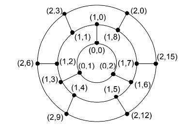
An eye network graph with \(s+1\) layers of concentric cycle [36]. It is represented by \(Eye\left(s\right).\) The \(s+1\) cycles can be written as \(l_{0},l_{1},l_{2},…,l_{s-1}\) and \(O_{s},\) here \(O_{s}\) represents the outermost cycle. The size, order and degree of eye networks are \(9\left(2^{s}-1\right)\) , \(6\left(2^{s}-1\right)\) and \(3\) respectively. Vertex and edge set of Eye networks are following
\[\begin{aligned} V\left(Eye\left(s\right)\right)&= \cup_{k=0}^{s-1} V\left(I_{k}\right)\cup V\left(O_{s}\right).\nonumber \\ V\left(I_{k}\right)&=\{\left(k,j\right)| 0\leq j \leq N_{k}-1 ; 0\leq k \leq s-1\}.\\ V\left(O_{s}\right)&= \{\left(s,j\right)| 0\leq j \leq N_{s}-1 ; 0\leq k \leq s-1 ~~ and ~~ |j|_{3}=0 \}.\\ E\left(Eye\left(s\right)\right)&=\cup_{k=0}^{s-1}E\left(I_{k}\right)\cup E\left(O_{s}\right)\cup\left(\cup_{k=o}^{s-1}E^{k+1}_{k}\right). \end{aligned}\] where \(N_k=9\times 2^{k-1}\) for positive \(k\) \[ e_{k,j}= \left\{ \begin{array}{ll} \left(\left(k,j\right),\left(k,j+1\right)\right) ; 0\leq j \leq N_{k}-1 \hspace{.1cm} and \hspace{.1cm} 0\leq k \leq s-1,\\ \left(\left(k,j\right),\left(k,j+3\right)\right) ; k=s \hspace{.1cm} and \hspace{.1cm} 0\leq j \leq N_s-1 \hspace{.1cm} and \hspace{.1cm} |j|_{3}=0.\\ \end{array} \right.\] \[e_{k,j}^{k+1}= \left\{ \begin{array}{ll} \left(\left(0,j\right),\left(1,2j+|j|_{3}\right)\right) ; k=0; j=0,1,2,…,\\ \left(\left(k,j\right),\left(k+1,2j+|j|_{3}\right)\right) ; |j|_{3}\neq 0 \hspace{.1cm} and \hspace{.1cm} 1\leq k \leq s-1 \hspace{.1cm},\\and \hspace{.1cm} 0\leq j \leq N_{k}-1.\\ \end{array} \right.\] The set \(\{e_{k,j} |~0\leq j \leq N_k-1\}\) is denoted by \(E(I_k)\) if \(0\leq k \leq s-1,\) and denoted by \(E(O_s)\) if \(k=s.\) We use \(E_k^{k+1}\) to denote the set \(\{e_{k,j}^{K+1} |~0\leq j \leq N_k-1\}.\) For better understanding of the labeling of Eye-networks following Figure is illustrated.
Theorem 13. Let \(\psi\) be the eye network, then Randić, general and reduced reciprocal Randić indices are
\[ \begin{aligned} &1:\ R_{\alpha}(\psi) &= 9^{\alpha+1}(2^s – 1).\\ &2:\ RR_{\alpha}(\psi) &= 9^{1-\alpha}(2^s – 1).\\ &3:\ RRR(\psi) &= 18(2^s – 1). \end{aligned} \]
Proof: The size and degree of Eye networks are \( 9(2^s – 1) \) and \( 3 \), respectively. Substituting these values into the formulas, we obtain the Randić family of indices:
\[ \begin{aligned} &1:\ R_{\alpha}(\psi) &= \sum_{uv \in E(\psi)}(d_u d_v)^{\alpha} = 9(2^s – 1)(3 \times 3)^{\alpha} \\ &&&= 9(2^s – 1)(9)^{\alpha} = 9^{\alpha+1}(2^s – 1). \\ &2:\ RR_{\alpha}(\psi) &= \sum_{uv \in E(\psi)}\frac{1}{(d_u d_v)^{\alpha}} = \frac{9(2^s – 1)}{(9)^{\alpha}} \\ &&&= 9^{1-\alpha}(2^s – 1). \\ &3:\ RRR(\psi) &= \sum_{uv \in E(\psi)}\sqrt{(d_u – 1)(d_v – 1)} = 9(2^s – 1)\sqrt{4} \\ &&&= 18(2^s – 1). \end{aligned} \]
Theorem 14. Let \(\psi\) be the eye network, then we have family of Zagreb indices are
\(M_{1}\left(\psi\right) ~~= 54\left(2^{s}-1\right),\)
\(M_{2}\left(\psi\right)~~= 81\left(2^{s}-1\right),\)
\(M_{3}\left(\psi\right) ~~= 0,\)
\(PM_{1}\left(\psi\right) = 6^{9\left(2^{s}-1\right)},\)
\(PM_{2}\left(\psi\right)=9^{9\left(2^{s}-1\right)},\)
\(AZI\left(\psi\right)\hspace{.05cm}=\frac{6561}{343}\left(2^{s}-1\right),\)
\(RM_2\left(\psi\right)=36\left(2^{s}-1\right),\)
\(^mM_2\left(\psi\right)=\left(2^{s}-1\right),\)
\(HM\left(\psi\right) =324\left(2^{s}-1\right).\)
Proof. The size and degree of Eye networks are \(9\left(2^{s}-1\right),\) 3 respectively, after putting these parameters into formulas we get Zagreb family of indices,
\[ \begin{aligned} &1:\ M_{1}(\psi) &= \sum_{uv \in E(\psi)}(d_u + d_v) = 9(2^s – 1)(6) = 54(2^s – 1). \\ &2:\ M_{2}(\psi) &= \sum_{uv \in E(\psi)}(d_u d_v) = 9(2^s – 1)(9) = 81(2^s – 1). \\ &3:\ M_{3}(\psi) &= \sum_{uv \in E(\psi)}(d_u – d_v) = 9(2^s – 1)(0) = 0. \\ &4:\ PM_{1}(\psi) &= \prod_{uv \in E(\psi)}(d_u + d_v) = 6^{9(2^s – 1)}. \\ &5:\ PM_{2}(\psi) &= \prod_{uv \in E(\psi)}(d_u d_v) = 9^{9(2^s – 1)}. \\ \end{aligned} \]
\[ \begin{aligned} &6:\ AZI(\psi) &= \sum_{uv \in E(\psi)}\left(\frac{d_u d_v}{d_u d_v – 2}\right)^3 = 9(2^s – 1)\left(\frac{9}{7}\right)^3 = \frac{6561}{343}(2^s – 1). \\ &7:\ RM_2(\psi) &= \sum_{uv \in E(\psi)}(d_u – 1)(d_v – 1) = 9(2^s – 1)(4) = 36(2^s – 1). \\ &8:\ ^mM_2(\psi) &= \sum_{uv \in E(\psi)}\frac{1}{d_u d_v} = 9(2^s – 1)\frac{1}{9} = 2^s – 1. \\ &9:\ HM(\psi) &= \sum_{uv \in E(\psi)}(d_u + d_v)^2 = 9(2^s – 1)(6^2) = 324(2^s – 1). \end{aligned} \]
Theorem 15. Let \(\psi\) be the eye network, then sum connectivity and general sum connectivity indices are
\[ \begin{aligned} &1:\ SCI(\psi) &= \frac{9}{\sqrt{6}}(2^s – 1). \\ &2:\ \chi_{\alpha}(\psi) &= 9(2^s – 1)6^{\alpha}. \end{aligned} \]
Proof: By using the size and degree of networks, \( 9(2^s – 1) \) and \( 3 \) respectively, the following indices can be computed as shown below:
\[ \begin{aligned} &1:\ SCI(\psi) &= \sum_{uv \in E(\psi)}\frac{1}{\sqrt{d_u + d_v}} = 9(2^s – 1)\frac{1}{\sqrt{6}} = \frac{9}{\sqrt{6}}(2^s – 1). \\ &2:\ \chi_{\alpha}(\psi) &= \sum_{uv \in E(\psi)}(d_u + d_v)^{\alpha} = 9(2^s – 1)6^{\alpha}. \end{aligned} \]
Theorem 16. Let \(\psi\) be the eye network, then geometric arithmetic, symmetric division and inverse sum indices are
\[ \begin{aligned} &1:\ GA(\psi) &= GA_5(\psi) = 9(2^s – 1). \\ &2:\ SDI(\psi) &= 18(2^s – 1). \\ &3:\ IS(\psi) &= \frac{27}{2}(2^s – 1). \end{aligned} \]
Proof: By using the size and degree of the networks, \( 9(2^s – 1) \) and \( 3 \) respectively, the following indices—Geometric Arithmetic (GA), Symmetric Division Index (SDI), and Inverse Sum Index (IS)—can be computed as shown below:
\[ \begin{aligned} &1:\ GA(\psi) &= \sum_{uv \in E(\psi)}\frac{2\sqrt{d_u d_v}}{d_u + d_v} = 9(2^s – 1)\frac{2\sqrt{9}}{6} = 9(2^s – 1). \\ &2:\ SDI(\psi) &= \sum_{uv \in E(\psi)}\frac{d_u^2 + d_v^2}{d_u d_v} = 9(2^s – 1)\frac{18}{9} = 18(2^s – 1). \\ &3:\ IS(\psi) &= \sum_{uv \in E(\psi)}\frac{d_u d_v}{d_u + d_v} = 9(2^s – 1)\frac{9}{6} = \frac{27}{2}(2^s – 1). \end{aligned} \]
Theorem 17. : Let \(\psi\) be the eye network, then different M-polynomials are:
\[ \begin{aligned} &1:\ M_{1}(\psi;x,y) &= 54(2^s – 1)(xy)^3. \\ &2:\ M_{2}(\psi;x,y) &= 729(2^s – 1)^2(xy)^6. \\ &3:\ mM(\psi;x,y) &= 9(2^s – 1)^2(xy)^6. \\ &4:\ R_{\alpha}(\psi;x,y) &= \left(729(2^s – 1)^2(xy)^6\right)^{\alpha}. \\ &5:\ RR_{\alpha}(\psi;x,y) &= 9(2^s – 1)^2(xy)^6. \\ &6:\ SDI(\psi;x,y) &= 162(2^s – 1)^2(xy)^6. \\ &7:\ H(\psi;x,y) &= 54(2^s – 1)^2 x^9 y^3. \\ &8:\ IS(\psi;x,y) &= 19683(2^s – 1)^3 x^{15} y^9. \end{aligned} \]
Proof. To get the results for the M-polynomials, following few formulas computed by using the definition of M-polynomials given in the form of differential in equation (8). \[\begin{aligned} D_{x}&=D_{y}=27\left(2^{s}-1\right)\left(xy\right)^{3},~~~~J=9\left(2^{s}-1\right)x^{6}.\nonumber\\ S_{x}&=S_{y}=3\left(2^{s}-1\right)\left(xy\right)^{3},~~~~Q_{-2}=9\left(2^{s}-1\right)xy^{3}.\nonumber \end{aligned}\] after plugging all above equations we get required following results.
\[ \begin{aligned} &1:\ M_1(\psi;x,y) &= \left(D_x + D_y\right)M(\psi;x,y) \\ &&= 27(2^s – 1)(xy)^3 + 27(2^s – 1)(xy)^3 \\ &&= 54(2^s – 1)(xy)^3. \\ &2:\ M_2(\psi;x,y) &= \left(D_x D_y\right)M(\psi;x,y) \\ &&= 27(2^s – 1)(xy)^3 \times 27(2^s – 1)(xy)^3 \\ &&= 729(2^s – 1)^2(xy)^6. \\ &3:\ ^mM(\psi;x,y) &= \left(S_x S_y\right)M(\psi;x,y) \\ &&= \left(3(2^s – 1)(xy)^3 \times 3(2^s – 1)(xy)^3\right) \\ &&= 9(2^s – 1)^2(xy)^6. \\ &4:\ R_\alpha(\psi;x,y) &= \left(D_x^\alpha D_y^\alpha\right)M(\psi;x,y) \\ &&= \left(27(2^s – 1)(xy)^3\right)^\alpha \times \left(27(2^s – 1)(xy)^3\right)^\alpha \\ &&= \left(729(2^s – 1)^2(xy)^6\right)^\alpha. \\ &5:\ RR_\alpha(\psi;x,y) &= \left(S_x^\alpha S_y^\alpha\right)M(\psi;x,y) \\ &&= \left(3(2^s – 1)(xy)^3\right)^\alpha \times \left(3(2^s – 1)(xy)^3\right)^\alpha \\ &&= \left(9(2^s – 1)^2(xy)^6\right)^\alpha. \\ &6:\ SDI(\psi;x,y) &= \left(D_x S_y + D_y S_x\right)M(\psi;x,y) \\ &&= 3(2^s – 1)(xy)^3 \times 27(2^s – 1)(xy)^3 + 27(2^s – 1)(xy)^3 \times 3(2^s – 1)(xy)^3 \\ &&= 162(2^s – 1)^2(xy)^6. \\ &7:\ H(\psi;x,y) &= 2S_x J M(\psi;x,y) \\ &&= 2 \times 3(2^s – 1)(xy)^3 \times 9(2^s – 1)x^6 \\ &&= 54(2^s – 1)^2 x^9 y^3. \\ &8:\ IS(\psi;x,y) &= S_x J D_x D_y M(\psi;x,y) \\ &&= 27(2^s – 1)(xy)^3 J \\ &&= 9(2^s – 1)x^6 \times 27(2^s – 1)(xy)^3 \times 27(2^s – 1)(xy)^3 \\ &&= 19683(2^s – 1)^3 x^{15} y^9. \end{aligned} \]
This completes the proof.
The exploration of computing M-polynomials and degree-based topological indices in different interconnection networks stands as a pivotal endeavor within the realm of network science. This pursuit is underscored by its inherent significance in unraveling the structural intricacies of complex networks, offering a nuanced understanding that extends beyond traditional metrics. The M-polynomials, derived from the characteristic polynomial of graphs, encapsulate essential information about the network’s topological features. This mathematical abstraction enables researchers to distill intricate network structures into concise representations, facilitating a more profound exploration of connectivity patterns and graph properties.
The implementation of this computational approach involves navigating the vast landscape of interconnection networks, ranging from classic architectures to modern communication networks. The computational methods utilized in this study transcend mere abstraction, providing a practical means to assess and characterize the connectivity patterns of diverse networks. This implementation allows for a detailed analysis of different interconnection network models, shedding light on their unique topological signatures and the implications of structural variations.
The significance of computing M-polynomials and degree-based topological indices is accentuated by their applications in diverse domains. In the context of communication networks, understanding the inherent connectivity structures becomes paramount for optimizing routing algorithms, enhancing fault tolerance, and improving overall network performance. Furthermore, in the realm of social networks, the insights garnered from these computations could illuminate patterns of influence and information flow, fostering a deeper comprehension of social dynamics.
Beyond theoretical implications, the applications extend to areas such as epidemiology, where the study of contact networks is crucial for modeling the spread of diseases. The ability to compute M-polynomials and degree-based indices provides a robust foundation for understanding the intricate relationships between individuals and predicting the potential impact of interventions on disease transmission dynamics.
In conclusion, the pursuit of computing M-polynomials and degree-based topological indices in different interconnection networks transcends the theoretical confines of graph theory. It offers a pragmatic lens through which to analyze, model, and optimize complex systems across diverse disciplines, imparting a wealth of knowledge with far-reaching implications in the realms of technology, communication, and societal understanding.
In this paper, we investigate the topological indices of different interconnection networks. We compute Randić index, general Randić index, sum connectivity index, families of Zagreb index, symmetric division index and geometric arithmetic indices. We also compute the M-polynomials of K-swapped networks of t-regular graphs, \(n\)-dimension tiwested cube and eye netwoks. Degree-based topological indices and M-polynomials are mathematical tools used in graph theory to analyze the structural properties of graphs, including interconnection networks. Interconnection networks are crucial components in various fields such as computer science, telecommunications, and social network analysis.
Different new indices are still open for above structures like, reverse-degree-based topological indices, such as the reverse-degree-based topological index of the first, second, and hyper Zagreb, forgotten, geometric arithmetic, atom-bond-connectivity, and the Randic index.