
Graph theory is a branch of mathematics that studies the properties and systems of graphs, which include vertices (or nodes) related via edges (or links). It performs a crucial role in modeling relationships and systems in numerous fields, such as computer science, biology, chemistry, social sciences, and engineering. A graph can be directed, where edges have a particular route, or undirected, wherein connections among vertices are bidirectional. Key standards in graph concepts include paths, cycles, connectivity, and graph coloring. Specialized topics like metric size, side metric size, and partitioning have wide packages, from community safety and verbal exchange structures to molecular chemistry and computational biology. The versatility of the graph principle permits it to be an effective device for studying each theoretical and practical troubles in complicated networks [1].
Resolvability parameters in graph theory refer to certain properties that allow for the distinction between vertices in a graph based on their distances to a selected subset of vertices, known as a resolving set. The most basic of these parameters is the metric dimension, which is the minimum number of vertices in a resolving set. Every vertex in the graph can be uniquely identified by its distance to the vertices in the set. It is introduced by P. J. Slater in \(1975\) [2] and later on by [3]. Blumenthal had already described the metric dimension and the rotating set [4]. After this the extension of this work is done by G. Chartrand in \(2000\) that is partition dimension [5] Another related parameter is the edge metric dimension, which focuses on uniquely distinguishing edges rather than vertices by using similar principles. It is introduced by A Kelenc in \(2018\) [6]. Extensions of these concepts include the mixed metric dimension, which simultaneously considers both vertices and edges in the graph and it is also introduced by A. Kelenc in \(2017\) [7]. These parameters are critical in understanding the structural complexity and uniqueness of graphs, as they provide a way to quantify how well the graph can be resolved or “mapped” by using a minimal set of references within the graph. Other parameters, Latter on the edge partition dimension introduced by I.G. Yero et. al in [8] and after this, in \(2024\) a novel resolvability parameter is introduced by Sikander Ali et. al [9], take a different approach by grouping vertices or edges into partitions that can still uniquely identify other elements in the graph based on distances. These resolvability parameters are key tools in the theoretical study of graphs, offering insight into their structure and distinguishability.
In this article, we discuss about local metric dimension and introduce a new parameter known as the local edge partition dimension. The local metric dimension of a graph is a variation of the classic metric dimension that focuses on resolving the neighborhoods of vertices, rather than the entire graph. Specifically, for a given vertex, the aim is to distinguish vertices within its local neighborhood based on their distances to a specific subset of vertices known as a local resolving set. A local resolving set for a vertex \(v\) is a set of vertices such that for any two distinct vertices in the neighborhood of \(v\), their distances to the vertices in the set uniquely identify them. The local metric dimension of the graph is the minimum number of vertices required in a resolving set to locally resolve all vertices in the graph. This concept is useful in scenarios where the focus is on distinguishing vertices within localized regions of the graph rather than the entire structure. It is introduced by F. Okamoto et, al [10]. A location partition dimension of a graph \(G\) is a partition of its vertex set into subsets \({P}_{1},{P}_{2},{P}_{3},\dots,{P}_{k}\) such that for any two distinct vertices uu and \(v\) in the graph, the distance from \(u\) and \(v\) to each subset is distinct. This means that for any pair of distinct vertices \(u\) and \(v\), the ordered tuple of distances from \(u\) to each subset \({P}_{i}\)(and similarly for \(v\)) should be different [11].
The local edge metric dimension of a graph is a variation of the edge metric dimension that focuses on distinguishing edges within the local neighborhood of a vertex. In this context, the goal is to uniquely identify the edges connected to a given vertex by using a subset of vertices, called a local edge resolving set [12]. The local edge partition dimension is the extension of the local edge partition dimension. Let \(R=\{{R}_{p1},{R}_{p2},{R}_{p3}\dots,{R}_{pi}\}\) be the set of subsets of vertices of \(G,\) and \({R}_{p1}\cup{R}_{p2}\cup{R}_{p3}\dots\cup{R}_{pi}=V(G),\) \({R}_{p1}\cap{R}_{p2}\cap{R}_{p3}\dots\cap{R}_{pi}=\emptyset\) then \({R}\) is said to be partition set of \(G\). Let \({R}\) show the unique representation with every pair(adjacent) of edges of \(G\) then \({R}\) is called the local edge resolving partition set and its minimum cardinality is known as the local edge partition dimension. It is introduced in this article and we apply the definition of path, cycle, and Petersen graph.
The concept of metric dimension finds applications in various fields and has been the subject of extensive research. The researchers have employed it in a wide range of applications, showcasing its versatility and importance. For instance, metric dimension has been used to determine similarities between different medications [13]. Metamaterials refer to artificially designed materials and structures [14], which is crucial in the pharmaceutical industry. Other applications include solving combinatorial optimization problems [15], facilitating robot navigation 16], addressing pharmaceutical chemistry issues [17], optimizing computer networks [18], and canonically labeling graphs [19]. The utility of metric dimension extends to solving location problems, aiding in the operation of sonar and coast guard Loran systems [20], facilitating image processing, and solving complex weighing problems [21]. Additionally, it has found applications in coding and decoding strategies for games like Mastermind [22]. The use of metric dimension in the development of city [23].
During the past 40 years, there has been a lot of research done on the metric dimension of various types of graphs. For instance constant time calculation of the metric dimension of the join of path graphs discussed in [24], the double resolvability parameters of Fosmidomycin anti-malaria drug and exchange property is studied in [25], metric dimensions of bicyclic graphs with potential applications in supply chain logistics studied in [26], double resolving set and exchange property in nanotube discussed in [27], metric dimensions of bicyclic graphs discussed by [28], the double edge resolving set and exchange property for nanosheet discussed in [29]. The concept of the metric dimension is applied to resolve a wide range of challenging issues due to its diversity. We mention [30-32] for the resolvability criteria of various chemical structures. Structural analysis of octagonal nanotubes via double edge-resolving partitions [33]. Mixed metric dimension and exchange property of hexagonal nano-network discussed in [34] and fault-tolerant basis of generalized fat trees and perfect binary tree derived architectures [35], fault-tolerance and unique identification of vertices and edges in a graph, the fault-tolerant mixed metric dimension studied by [36], and Redefining fractal cubic networks and determining their metric dimension and fault-tolerant metric dimension discussed in [37] and in other field see [38]. Fault-tolerant metric dimensions of leafless cacti graphs with application in supply chain management [39]. The concept of metric dimension has been applied to solve challenging problems in various contexts. The resolving set of silicate stars was explored in a publication by George [40]. Cellulose networks’ upper bounds for metric dimension were determined in research conducted by [41]. The discussion on the graph of convex polytopes was presented in a work by [42].
Definition 1. Let \(N(v)\) be the neighborhood of a vertex \(v \in V\), i.e., the set of all vertices adjacent to \(v\), formally: \[N(v) = \{ u \in V : uv \in E \}.\] A set of vertices \(S \subseteq V\) is called a local resolving set for \(v\) if for any two distinct vertices \(u, w \in N(v)\), there exists a vertex \(s \in S\) such that the distance from \(u\) to \(s\), denoted \(d(u, s)\), is different from the distance from \(w\) to \(s\) [10], i.e., \[d(u, s) \neq d(w, s).\]
Definition 2. The local partition dimension [11] of a graph \(G = (V, E)\) is defined as follows:
Let \(N(v)\) be the open neighborhood of a vertex \(v \in V\), defined as the set of vertices adjacent to \(v\): \[N(v) = \{ u \in V : uv \in E \}.\]
A partition \(\Pi = \{P_1, P_2, \dots, P_k\}\) of the vertex set \(V\) is called a local resolving partition for a vertex \(v \in V\) if for any two distinct vertices \(u, w \in N(v)\), the distance between \(u\) and each partition set \(P_i\) differs from the distance between \(w\) and each partition set \(P_i\). That is, for each pair of distinct vertices \(u, w \in N(v)\), there exists a partition \(P_i \in \Pi\) such that: \[d(u, P_i) \neq d(w, P_i),\] where \(d(x, P_i) = \min\{d(x, z) : z \in P_i\}\) is the minimum distance from vertex \(x\) to any vertex in \(P_i\).
The local partition dimension of the graph \(G\), denoted as \(\text{LPD}(G)\), is the minimum number of partitions required to form a local resolving partition for each vertex \(v \in V\). Formally: \[\text{LPD}(G) = \min \left\{ k : \Pi = \{P_1, P_2, \dots, P_k\} \text{ is a local resolving partition for each } v \in V \right\}.\]
Definition 3. The local edge metric dimension 43] of a graph \(G = (V, E)\) is defined as follows:
Let \(N(v)\) be the open neighborhood of a vertex \(v \in V\), defined as the set of vertices adjacent to \(v\): \[N(v) = \{ u \in V : uv \in E \}.\]
A set of vertices \(S \subseteq V\) is called a local edge resolving set for \(v\) if for any two distinct edges \(uv, vw\) incident to \(v\), there exists a vertex \(s \in S\) such that the distance from the endpoints of the edges to \(s\) differs. That is, for the edges \(uv\) and \(vw\), we have: \[d(u, s) \neq d(v, s) \quad \text{and} \quad d(v, s) \neq d(w, s).\]
The local edge metric dimension of the graph \(G\), denoted as \(\text{LEMD}(G)\), is the minimum size of a local edge resolving set that can distinguish all incident edges at each vertex \(v \in V\). Formally: \[\text{LEMD}(G) = \min \left\{ |S| : S \subseteq V \text{ is a local edge resolving set for each vertex } v \in V \right\}.\]
Definition 4. The local edge partition dimension of a graph \(G = (V, E)\) is defined as follows:
Let \(N(v)\) be the neighborhood of a vertex \(v \in V\), defined as the set of vertices adjacent to \(v\): \[N(v) = \{ u \in V : uv \in E \}.\]
A partition \(\Pi = \{P_1, P_2, \dots, P_k\}\) of the vertex set \(V\) is called a local resolving partition for a vertex \(v \in V\) if for any two distinct edges \(u, w \in N(E)\), the distance between \(u\) and each partition set \(P_i\) differs from the distance between \(w\) and each partition set \(P_i\). That is, for each pair of distinct vertices \(u, w \in N(v)\), there exists a partition \(P_i \in \Pi\) such that: \[d(u, P_i) \neq d(w, P_i),\] where \(d(x, P_i) = \min\{d(x, z) : z \in P_i\}\) is the minimum distance from edge \(x\) to any vertex in \(P_i\).
The local edge partition dimension of the graph \(G\), denoted as \(\text{LEPD}(G)\), is the minimum number of partitions required to form a local edge resolving partition for each vertex \(v \in V\). Formally: \[\text{LEPD}(G) = \min \left\{ k : \Pi = \{P_1, P_2, \dots, P_k\} \text{ is a local edge resolving partition for each } v \in V \right\}.\]
In this section, we discussed novel resolvability parameters, the local edge partition dimension of the path, cycle, and Petersen graph, the local metric dimension of the cycle for even and odd lengths, and other resolvability parameters of the Petersen graph.

Theorem 5. The local edge partition dimension of a graph \(G\) is \(2\) if and only if \(G=P_{n}\).
Proof. We begin by noting that \(\text{lepd}(P_n) = 2\), which can be demonstrated by dividing the vertices of \(P_n\) into two groups: one set containing a single leaf, and the other set containing the remaining vertices. Now, let’s consider a graph \(G\) where \(\text{lepd}(G) = 2\), and assume \({V_1, V_2}\) forms an local edge-resolving partition set. If there exist two edges, \(m = pq\) and \(n = st\), such that without loss of generality, \(p,s \in V_1\) and \(q, t \in V_2\), then the distances \(d(m, V_1) = d(m, V_2) = d(n, V_1) = d(n, V_2)\) would all be zero, which is a contradiction. Therefore, since \(G\) is a connected graph, there must be exactly one edge, say \(h = q_1q_2\), where \(q_1 \in V_1\) and \(q_2 \in V_2\).
Next, assume the maximum degree of \(G\) is at least \(3\). Let \(w\) be the closest vertex to \(q_1\) with the highest degree, and suppose \(u \in V_1\). Consider two vertices adjacent to \(u\), labeled \(u_1\) and \(u_1'\), that also belong to \(V_1\) and are not part of the shortest path between \(V_1\) and \(u\). Under these conditions, the edges \(uu_1\) and \(uu_1'\) would result in \(d(uu_1, V_2) = d(uu_1, V_1) + 1\) and \(d(uu_1', V_2) = d(uu_1', V_1) + 1\). This creates a contradiction, implying that the maximum degree of \(G\) must be no greater than \(2.\) If \(G\) were a cycle, any partition of its vertices into two sets would generate at least two edges with one endpoint in each set, which is not feasible. Consequently, \(G\) must be a path, thus completing the proof. ◻
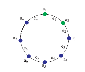
A cycle graph is also a simple graph in graph theory it is denoted by \(C_{n}\) where \(n\geq 3.\) It is defined as, a closed walk in which all the vertices are different except \(({a_{n}}={a_{1}})\) is called a cycle graph. The total number of vertices is \(n\) and the total number of edges is also \(n\) and the vertex and edge set is defined as \[\begin{aligned} &V(C_{n})=\{{a_{i+1}}; 1\leq{i}\leq{n}\} \\ &E(C_{n})=\{{a_{i}}{a_{i+1}}, {a_{n}{a_{1}}}; 1\leq{i}\leq{n}, \}\\ \end{aligned}\]
Theorem 6. The local edge partition dimension of cycle graph \(C_{n}\) is \(3,\) where \(n\geq 3\).
Proof. Assume that a subset of the vertices of \({C}_{n}\) is \({R}=\{{R}_{p1},{R}_{p2},{R}_{p3}\}\) where
\({R}_{p1}=\{{a}_{1}\},\) \({R}_{p2}=\{{a}_{2}\},\) and \({R}_{p3}= V({C}_{n})\backslash
\{{a}_{1},{a}_{2}\}.\) We shall demonstrate that \(R\) is a local edge partition resolving set
to demonstrate that \(lepd({C}_{n})\leq3\). The distinct
representations of all the edges of \({C}_{n}\) in Table 1
are shown below.
The representation of \(R=\{ a_{1},
a_{2}, a_{n}\}\) for \({n \geq
3}\) present in Table 1
| \(r(. \mid R )\) | \( (R_p1,R_p2,R_p3) \) |
| \(e_1\) | (0, , 1) |
| \(e_2\) | (1, 0, 0) |
| \(e_3\) | (2, 1, 0) |
| \(e_4\) | (3, 2, 0) |
| \(e_5\) | (4, 3, 0) |
| . | . |
| . | . |
| . | . |
| \(e_n-1\) | (1, 2, 0) |
| \(e_n\) | (0, 1, 0) |
From Table 1 it is clear that the \(R\) has unique representation with all edges of \(C_{n}\) so \(R\) is local edge partition resolving set of cardinality \(3.\)
The generalized formulas for all edges of the cycle graph show that the local edge partition dimensions are \(3\) because all adjacent edges are distinct. Let \(\eta\) be the distance’s symbol. Let \(\eta(e_{i}, {R}_{p1}) =w^{\prime}_{1},\ \eta(e_{i},{R}_{p2}) =w^{\prime}_{2}, \ \eta(e_{i},\ {R}_{p3}) =w^{\prime}_{3},\) and \(r({a}_{i}\mid R)=({w}_{1}^{\prime}, \ {w}_{2}^{\prime},\ {w}_{3}^{\prime})\) \[\begin{aligned} {w}_{1}^{\prime} = \left\lbrace \begin{array}{ll} {i}-1 &\hbox{for} \ 1\leq{i}\leq \left\lceil\frac{{n}}{2}\right\rceil, \\ {n}-{i} &\hbox{for} \ \left\lceil\frac{{n}}{2}\right\rceil < {i}\leq {n},\\ \end{array} \right. \end{aligned}\] \[\begin{aligned} {w}_{2}^{\prime} = \left\lbrace \begin{array}{ll} 0 & \hbox{for} \ i= 1,\\ {i}-2 &\hbox{for} \ 1\leq{i}\leq \left\lceil\frac{{n}}{2}\right\rceil +1, \\ {n}-{i}+1 &\hbox{for} \ \left\lceil\frac{{n}}{2}\right\rceil +1 < {i}\leq {n},\\ \end{array} \right. \end{aligned}\] \[\begin{aligned} {w}_{3}^{\prime} = \left\lbrace \begin{array}{ll} {1} &\hbox{for} \ {e}_{1}\\ 0 & \hbox{otherwise} \\ \end{array} \right. \end{aligned}\] The minimum cardinality of \(R\) is the local edge partition dimension so the local edge partition dimension of \({C}_{n}\) is \(3.\) From all the above discussion it is clear that the metric dimension of \({C}_{n}\) is less or equal to \(3.\) Now we are going to prove that the local edge partition dimension of \({C}_{n}\) is not less than \(3.\) The local edge partition dimension \(2\) is possible only in the case of a path graph see Theorem 5. Hence the the local edge partition dimension of \({C}_{n}\) is \(3.\) ◻
Theorem 7. The local metric dimension of cycle graph \(C_{n}\) is \(2\) where \(n\) is odd.
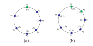
Proof. Let \({R}=\{{a_{1}}\}\) be the subset of the vertices of \({C}_{n}\) in Figure 3(a). We note that the distance of \({a}_{4}\) and \({a}_{5}\) are the same and both are adjacent so \({R}\) is not a local resolving set. We want to prove that the \({R}\) is a local resolving so \(R\) must have a unique representation with all adjacent vertices of \({C}_{n}.\) In general we can say that if we take the cardinality of \({R}\) is one then the representation of two adjacent vertices \({a}_{\frac{n+1}{2}}\) and \({a}_{\frac{n+3}{2}}\) remain same. In Figure 3(b) we note that \({a}_{\frac{n+1}{2}}\) and \({a}_{\frac{n+3}{2}}\) have unique representation with \({R}=\{{a_{1},{a}_{2}}\}\) and all other adjacent vertices of odd cycle when \({R}\) has cardinality \(2\). So \({R}\) is the local resolving set and the minimum cardinality of the local resolving set is the local metric dimension. Hence the local metric dimension of cycle graph \({C}_{n}\) is two when \({n}\) is odd. Let \(\eta\) be the distance’s symbol. Let \(\eta(a_{i}, a_{1}) =w_{1},\eta(a_{i}, a_{2}) =w_{2}, \eta(a_{i}, a_{n}) =w_{3},\) and \(r({a}_{i}\mid R)=({w}_{1}, {w}_{2}, {w}_{3}).\) \[\begin{aligned} {w}_{1} = \left\lbrace \begin{array}{ll} {i}-1 &\hbox{for} \ 1\leq{i}\leq \left\lceil\frac{{n}}{2}\right\rceil, \\ {n}-{i}+1 &\hbox{for} \ \left\lceil\frac{{n}}{2}\right\rceil < {i}\leq {n},\\ \end{array} \right. \end{aligned}\]
\[\begin{aligned} {w}_{2} = \left\lbrace \begin{array}{ll} 1 & \hbox{for} \ i= 1,\\ {i}-2 &\hbox{for} \ 1\leq{i}\leq \left\lceil\frac{{n}}{2}\right\rceil +1, \\ {n}-{i}+2 &\hbox{for} \ \left\lceil\frac{{n}}{2}\right\rceil +1 < {i}\leq {n},\\ \end{array} \right. \end{aligned}\] ◻
Theorem 8. The local metric dimension of a complete bipartite graph also is \(1\).
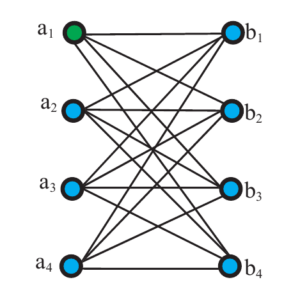
Proof. Suppose \({R}=\{{a_{1}}\}\) be the subset of the vertices of \({K}_{m,n}\). We want to prove that the \({R}\) is a local resolving set so \(R\) must have a unique representation with all adjacent vertices of \({K}_{m,n}.\) In Figure 4 we note that all adjacent vertices have unique distance from \({a}_{1}\) because all \({a}_{i}\) vertices have distance \(2\) with \({a}_{1}\) but all are non-adjacent. All \({b}_{i}\) have \(1\) distance from \({a}_{1}\) because all are attached with \({a}_{1}\) but these are also non-adjacent and \({R}=\{{a_{1}}\}\) so \({R}\) has unique representation. Hence \({R}\) is the local resolving set and the minimum cardinality of the local resolving set is the local metric dimension. Hence the local metric dimension of the bipartite graph is one. ◻
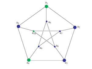
Theorem 9. The local metric dimension of the Petersen graph is \(3\).
Proof.
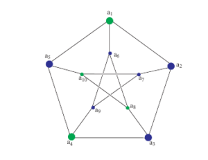
We want to prove that \(R_{l}=\{{a}_{1}, {a}_{4}, {a}_{10}\}\) is the local resolving set of minimum cardinality. Let \({R}_{l}\) be the subset of the vertices of the Petersen graph and the representation of all vertices of the graph is present in Table 2.
\(R_{l}=\{{a}_{1}, {a}_{4},
{a}_{10}\}\)
| \(vertex\) | \(a_1\) | \( a_2\) | \( a_3 \) | \(a_4\) | \(a_5\) |
| \(r(. \mid {R}_l)\) | (0,2,2) | (1,2,2) | (2,2,1) | (2,2,0) | (1,1,1) |
| \(vertex\) | \(a_6\) | \(a_7\) | \(a_8 \) | \(a_9 \) | \(a_10 \) |
| \(r(. \mid {R}_l )\) | (1,2,2) | (2,1,2) | (2,1,2) | (2,2,1) | (2,0,2) |
Table 2 is the avoidance that the representation of adjacent vertices is unique so \({R}_{l}\) is a local resolving set of cardinality \(3\) and \({R}_{l}\) is the set of minimum cardinality that show unique coding for each vertex. Hence the local metric dimension of the Petersen graph is \(3.\) ◻
Theorem 10. The local edge metric dimension of the Petersen graph is \(4\).
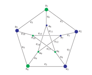
Proof. Let \({R}_{le}=\{{a}_{1}, {a}_{4}, {a}_{9},{a}_{10}\}\) be the subset of the vertices of Petersen graph and we want to show that it is an edge resolving set. The representation of all edges of the graph is present in Table 5.

\({R}_{le}=\{{a}_{1}, {a}_{4},
{a}_{9},{a}_{10}\}\)
| \(Edges\) | \(e_1\) | \( e_2\) | \( e_3 \) | \(e_4\) | \(e_5\) |
| \(r(. \mid {R}_le)\) | (0,2,1,2) | (1,1,2,2) | (2,0,2,2) | (1,0,2,1) | (0,1,1,1) |
| \(Edges\) | \(e_6\) | \(e_7\) | \(e_8 \) | \(e_9 \) | \(e_10 \) |
| \(r(. \mid {R}_le )\) | (0,2,0,2) | (1,2,2,1) | (2,1,1,1) | (2,0,1,2) | (1,1,2,0) |
| \(Edes\) | \(e_11\) | \(e_12\) | \(e_13 \) | \(e_14 \) ) | \(e_15 \) |
| \(r(. \mid {R}_le )\) | (1,2,0,1) | (1,2,0,1) | (2,2,1,0) | (1,1,0,2) | (2,2,2,0) |
From 3 it is clear that the representation of adjacent edges is unique so \({R}_{le}\) is the local edge resolving set of cardinality \(4\) and \({R}_{le}\) is the set of minimum cardinality that show unique coding for adjacent edges. Hence the local edge metric dimension of the Petersen graph is \(4.\) ◻
Theorem 11. The metric dimension of the Petersen graph is \(4\).
Proof. Suppose \({R}=\{{a}_{1}, {a}_{4}, {a}_{8},{a}_{10}\}\) be the subset of the vertices of Petersen graph and we want to show that it is a resolving set. The representation of all vertices of the graph is present in Table 4.
\({R}=\{{a}_{1}, {a}_{4},
{a}_{10},{a}_{8}\}\)
| \(vertex\) | \(a_1\) | \( a_2\) | \( a_3 \) | \(a_4\) | \(a_5\) |
| \(r(. \mid {R})\) | (0,2,2,2) | (1,2,2,2) | (2,1,1,2) | (2,0,2,2) | (1,1,2,2) |
| \(vertex\) | \(a_6\) | \(a_7\) | \(a_8 \) | \(a_9 \) | \(a_10 \) |
| \(r(. \mid {R} )\) | (1,2,1,2) | (2,2,2,1) | (2,2,1,0) | (2,1,2,2) | (2,2,0,1) |
From Table 4 it is clear that the representation is unique so \({R}\) is resolving set of cardinality \(4\) and \({R}\) is the set of minimum cardinality that shows unique coding for each vertex. Hence the metric dimension of the Petersen graph is \(4.\) ◻
Theorem 12. The edge metric dimension of the Petersen graph is \(5\).
Proof.
Let \({R}_{e}=\{{a}_{1}, {a}_{4},{a}_{8}, {a}_{9},{a}_{10}\}\) be the subset of the vertices of Petersen graph and we want to show that it is an edge resolving set. The representation of all edges of the graph is present in Table 5.
\({R}_{e}=\{{a}_{1}, {a}_{4},{a}_{8},
{a}_{9},{a}_{10}\}\)
| \(Edges\) | \(e_1\) | \( e_2\) | \( e_3 \) | \(e_4\) | \(e_5\) |
| \(r(. \mid {R}_e)\) | (0,2,2,1,2) | (1,1,1,2,2) | (2,0,1,1,2) | (1,0,2,1,1) | (0,1,2,2,1) |
| \(Edges\) | \(e_6\) | \(e_7\) | \(e_8 \) | \(e_9 \) | \(e_10 \) |
| \(r(. \mid {R}_e )\) | (0,2,1,1,2) | (1,2,2,2,1) | (2,1,0,2,1) | (2,0,2,1,2) | (1,1,1,2,0) |
| \(Edes\) | \(e_11\) | \(e_12\) | \(e_13 \) | \(e_14 \) | \(e_15 \) |
| \(r(. \mid {R}_e )\) | (1,2,0,1,1) | (2,1,2,0,1) | (2,2,0,2,0) | (1,1,1,0,2) | (2,2,1,2,0) |
Table 5 shows that the representation of edges is unique so \({R}_{e}\) is edge resolving set of cardinality \(5\) and \({R}_{e}\) is the set of minimum cardinality that show unique coding for each edge. Hence the edge metric dimension of the Petersen graph is \(5.\) ◻
Theorem 13. The local partition dimension of the Petersen graph is \(4\).
Proof. \({R}_{p1}={a}_{1}, {R}_{p2}={a}_{4}, {R}_{p3}={a}_{10}, {R}_{p4}=\{{a}_{2},{a}_{3}, {a}_{5},{a}_{6},{a}_{7}, {a}_{8},{a}_{9}\}\) and \({R}_{p}=\{{R}_{p1}, {R}_{p2}, {R}_{p3}, {R}_{p4}\}.\) \({R}_{p}\) is the set of the subset of the vertices of the Petersen graph and we want to show that it is a local partition resolving set. The representations of all adjacent vertices of the graph are present in Table 6.
\({R}_{lp}=\{{R}_{p1}, {R}_{p2}, {R}_{p3},
{R}_{p4}\}\)
| \(vertex\) | \(a_1\) | \( a_2\) | \(a_3 \) | \(a_4\) | \(a_5\) |
| \(r(. \mid {R}_lp)\) | (0,2,2,1) | (1,2,2,0) | (2,2,0) | (2,2,0,1) | (1,1,1,0) |
| \(vertex\) | \(a_6\) | \(a_7\) | \(a_8 \) | \(a_9 \) | \(a_10 \) |
| \(r(. \mid {R}_lp )\) | (1,2,2,0) | (2,1,2,0) | (2,1,2,0) | (2,2,1,0) | (2,0,2,1) |
Table 6 shows that the representation of adjacent vertices is unique so \({R}_{p}\) is the local partition resolving set of cardinality \(4\) and \({R}_{p}\) is the set of minimum cardinality that show unique coding for each adjacent vertices. Hence the partition metric dimension of the Petersen graph is \(4.\) ◻
Theorem 14. The local edge partition dimension of the Petersen graph is \(5\).
Proof. \({R}_{p1}={a}_{1}, {R}_{p2}={a}_{4}, {R}_{p3}={a}_{9}, {R}_{p4}={a}_{10}, {R}_{p5}=\{{a}_{2},{a}_{3}, {a}_{5},{a}_{6}, {a}_{7},{a}_{8}\}\) and \({R}_{lep}=\{{R}_{p1}, {R}_{p2}, {R}_{p3}, {R}_{p4}, {R}_{p5}\}.\) \({R}_{p}\) is the set of the subset of the vertices of the Petersen graph and we want to show that it is a local partition edge resolving set. The representations of all edges of the graph are present in Table 7.
\({R}_{lep}=\{{R}_{p1}, {R}_{p2}, {R}_{p3},
{R}_{p4}, {R}_{p5}\}\)
| \(Edges\) | \(e_1\) | \( e_2\) | \( e_3 \) | \(e_4\) | \(e_5\) |
| \(r(. \mid {R}_lep)\) | (0,2,1,2,0) | (1,1,2,2,0) | (2,0,2,2,0) | (1,0,2,1,0) | (0,1,1,1,0) |
| \(Edges\) | \(e_6\) | \(e_7\) | \(e_8 \) | \(e_9 \) | \(e_10 \) |
| \(r(. \mid {R}_lep )\) | (0,2,0,2,1) | (1,2,2,1,0) | (2,1,1,1,0) | (2,0,1,2,0) | (1,1,2,0) |
| \(Edes\) | \(e_11\) | \(e_12\) | \(e_13 \) | \(e_14 \) | \(e_15 \) |
| \(r(. \mid {R}_lep )\) | (1,2,0,1,0) | (1,2,0,1,0) | (2,2,1,0,0) | (1,1,0,2,0) | (2,2,2,0,0) |
From 7 it is clear that the representation of adjacent edges is unique so \({R}_{lep}\) is the local edge resolving set of cardinality \(5\) and \({R}_{lep}\) is the set of minimum cardinality that show unique coding for adjacent edges. Hence the local edge metric dimension of the Petersen graph is \(5.\) ◻
Theorem 15. The partition dimension of the Petersen graph is \(5\).
Proof. \({R}_{p1}={a}_{1}, {R}_{p2}={a}_{4}, {R}_{p3}={a}_{8}, {R}_{p4}={a}_{10}, {R}_{p5}=\{{a}_{2},{a}_{3}, {a}_{5},{a}_{7}, {a}_{8},{a}_{9}\}\) and \({R}_{p}=\{{R}_{p1}, {R}_{p2}, {R}_{p3}, {R}_{p4}, {R}_{p5}\}.\) \({R}_{p}\) is the set of a subset of the vertices of the Petersen graph and we want to show that it is a partition-resolving set. The representations of all vertices of the graph are present in Table 8.
\({R}_{p}=\{{R}_{p1}, {R}_{p2}, {R}_{p3},
{R}_{p4}, {R}_{p5}\}.\)
| \(vertex\) | \(a_1\) | \( a_2\) | \( a_3 \) | \(a_4\) | \(a_5\) |
| \(r(. \mid {R})\) | (0,2,2,2,1) | (1,2,2,2,0) | (2,1,1,2,0) | (2,0,2,2,1) | (1,1,2,2,0) |
| \(vertex\) | \(a_6\) | \(a_7\) | \(a_8 \) | \(a_9 \) | \(a_10 \) |
| \(r(. \mid {R} )\) | (1,2,1,2,1) | (2,2,2,1,0) | (2,2,1,0,0) | (2,1,2,2,9) | (2,2,0,1,1) |
From Table 8 it is clear that the representation is unique so \({R}_{p}\) is the partition resolving set of cardinality \(5\) and \({R}_{p}\) is the set of minimum cardinality that show unique coding for each vertex. Hence the partition dimension of the Petersen graph is \(5.\) ◻
Theorem 16. The edge partition dimension of the Petersen graph is \(6\).
Proof. suppose \({R}_{p1}={a}_{1}, {R}_{p2}={a}_{4}, {R}_{p3}={a}_{8}, {R}_{p4}={a}_{9}, {R}_{p5}={a}_{10}, {R}_{p6}=\{{a}_{2},{a}_{3}, {a}_{5},{a}_{7}, {a}_{8}\}\) and \({R}_{pe}=\{{R}_{p1}, {R}_{p2}, {R}_{p3}, {R}_{p4}, {R}_{p5},{R}_{p6}\}.\) \({R}_{pe}\) be the set of subset of the vertices of Petersen graph and we want to show that it is a partition edge resolving set. The representations of all edges of the graph are present in Table 9.
\({R}_{pe}=\{{R}_{p1}, {R}_{p2}, {R}_{p3},
{R}_{p4}, {R}_{p5},{R}_{p6}\}\)
| \(Edges\) | \(e_1\) | \( e_2\) | \( e_3 \) | \(e_4\) | \(e_5\) |
| \(r(. \mid {R}_pe)\) | (0,2,2,1,2,0) | (1,1,1,2,2,0) | (2,0,1,1,2) | (1,0,2,1,1,0) | (0,1,2,2,1) |
| \(Edges\) | \(e_6\) | \(e_7\) | \(e_8 \) | \(e_9 \) | \(e_10 \) |
| \(r(. \mid {R}_pe )\) | (0,2,1,1,2,0) | (1,2,2,2,1) | (2,1,0,2,1,0) | (2,0,2,1,2,0) | (1,1,1,2,0) |
| \(Edes\) | \(e_11\) | \(e_12\) | \(e_13 \) | \(e_14 \) | \(e_15 \) |
| \(r(. \mid {R}_pe )\) | (1,2,0,1,1,0) | (2,1,2,0,1) | (2,2,0,2,0,0) | (1,1,1,0,2,0) | (2,2,1,2,0) |
Table 9 shows that the representation of edges is unique so \({R}_{pe}\) is edge resolving set of cardinality \(5\) and \({R}_{pe}\) is the set of minimum cardinality that show unique coding for each edge. Hence the edge metric dimension of the Petersen graph is \(5.\) ◻
This article presents a comprehensive analysis of the Petersen graph through the lens of various resolvability parameters, including the novel local edge partition dimension. By calculating and comparing dimensions such as local metric, local edge metric, metric, edge metric, local partition, local edge partition, partition, and edge partition dimensions, we identified distinct structural characteristics that highlight the versatility of the Petersen graph as a model for complex networks. The inclusion of the local edge partition dimension offers a refined perspective on graph resolvability, contributing to a more nuanced understanding of connectivity and distance-based measures within graph theory. These insights not only enhance the theoretical foundation of resolvability parameters.
| Resolvability parameters | Graphs | Values |
| Local metric dimension | Petersen | 3 |
| Local edge metric dimension | Petersen | 4 |
| Metric dimension | Petersen | 4 |
| Edge metric dimension | Petersen | 5 |
| Local partition dimension | Petersen | 4 |
| Local edge partition dimension | Petersen | 5 |
| Partition dimension | Petersen | 5 |
| Edge partition dimension | Petersen | 6 |
| Local partition dimension | Petersen | 4 |
| Local metric dimension | cycle (even order) | 1 |
| Local metric dimension | cycle (odd order) | 2 |
| Local metric dimension | complete bipartite | 1 |
| Local edge partition dimension | cycle | 3 |
Is it feasible to define the mixed local partition dimension for a simple, undirected, connected graph?
I would like to express my heartfelt gratitude to my family and
friend (Muhammad Azeem) for their unwavering support,
encouragement, and understanding throughout the course of this research.
Their belief in me has been a constant source of strength and
motivation.