
Let \(0<k\in\mathbb{Z}\), let \(n=2k+1\) and let \(O_k\) be the \(k\)-odd graph [1], namely the graph whose vertices are the \(k\)-subsets of the cyclic group \(\mathbb{Z}_n\) over the set \([0,2k]=\{0,1,\ldots, 2k\}\) and having an edge \(uv\) for each two vertices \(u,v\) if and only if \(u\cap v=\emptyset\). The characteristic vectors of such subsets \(u,v\) of \([0,2k]\) are the \(n\)-vectors \(\vec{u},\vec{v}\) over \(Z_2\) whose supports (i.e, the subsets of \([0,2k]\) composed by all nonzero entries of \(u,v\)), are exactly \(u,v\), respectively. We may write \(\vec{u},\vec{v}\in V(O_k)\), instead of \(u,v\in V(O_k)\). The set \(V(O_k)\) of vertices of \(O_k\) admits a partition into cyclic classes mod \(n\), where two vertices \(\vec{u},\vec{v}\) are in the same class if and only if they are related by a translation mod \(n\), e.g., if \(\vec{u}=u_0\cdots u_{2k}\), then \(\vec{v}=u_iu_{i+1}\cdots u_{2k}u_0u_1\cdots u_{i-1}\), for some \(i\in\mathbb{Z}_n=[0,2k]\). This is a translation that we denote by \(i\in\mathbb{Z}_n\). The said cyclic classes mod \(n\) are to be optionally used in our final result, Corollary 5.
We also consider the double covering graph \(M_k\) of \(O_k\), where \(M_k\), referred to as middle-levels graph, is the subgraph of the Boolean lattice of subsets of \([0,2k]\) induced by the levels \(L_k\) (\(=V(O_k)\)) and \(L_{k+1}\), formed by the binary \(n\)-strings of weight \(k\) and \(k+1\), respectively [2-4]. Two vertices \(u\in L_k\) and \(v\in L_{k+1}\) of \(M_k\) are adjacent in \(M_k\) if and only if \(u\subset v\), with \(u\) and \(v\) taken as subsets of \([0,2k]\). The double-covering graph map \(\Theta:M_k\rightarrow O_k\) restricts to the identity map over \(L_k\) and to the reversed complement bijection \(\aleph\) over \(L_{k+1}\), that is: if \(v\in L_{k+1}\) has characteristic vector \(\vec{v}=v_0v_1\cdots v_{2k-1}v_{2k}\), then \(\Theta(v)=\aleph(v)\) has characteristic vector \(\bar{v}_{2k}\bar{v}_{2k-1}\cdots\bar{v}_1\bar{v}_0\) in \(V(O_k)\), where \(\bar{0}=1\) and \(\bar{1}=0\). To the partition of \(V(O_k)\) into cyclic classes mod \(n\), or \(\mathbb{Z}_n\)-classes, corresponds a partition of \(V(M_k)=L_k\cup L_{k+1}\) into dihedral classes, or \(\mathbb{D}_n\)-classes, where \(\mathbb{D}_n\supset\mathbb{Z}_n\) is the dihedral group of order \(2n\).
An \(n\)-string \(\Psi=0\psi_1\cdots\psi_{2k}\) in the alphabet \([0,n]\) in which each nonzero entry appears exactly twice is seen as a concatenation \(W^i|X|Y|Z^i\) of substrings \(W^i,X,Y\) and \(Z^i\), where \(W^i\) and \(Z^i\) have length \(i\), for some \(0<i<k\). In that case, the \(n\)-string \(W^i|Y|X|Z^i\) is said to be a \(i\)-nested castling of \(\Psi\) (time-consuming as it swaps parts of \(\Psi\), with many position changes).
A \(k\)-factor of a graph \(G\) is a spanning \(k\)-regular subgraph. A \(k\)-factorization is a partition of \(E(G)\) into disjoint \(k\)-factors. A 2-factor (or cycle factor [5]) in \(O_k\) formed by \(n\)-cycles, with a pullback 2-factor in \(M_k\) of \(2n\)-cycles via \(\Theta^{-1}\), and used in constructing Hamilton cycles [6] and optionally in Corollary 5 below, was analyzed in [4] from the viewpoint of restricted growth strings (RGS’s [7]), which form the RGS-tree \(\mathcal T\) of Lemma 1, below.
In Section 2, a modification of the arguments of [4] shows that such RGS’s exert control over the Dyck paths of length \(n\), that represent bijectively the cyclic (resp., dihedral) classes of vertices of \(O_k\) (resp., \(M_k\)). These paths, viewed as Dyck nests, defined in Subsection 4.1, were related via the (time-consuming) \(i\)-nested castling operation controlled by the RGS-tree \(\mathcal T\) that yields each non-root Dyck nest from its parent nest ([2-4], or Theorem 1) in the reinterpretation of the Hamilton cycle constructions in \(O_k\) [6] and \(M_k\) [8,9].
Such RGS-control will be reduced below, first by viewing each Dyck nest as its signature, defined in Subsection 5.2 and shown to be equivalent to that Dyck nest in Theorem 4, and second by collapsing each \(i\)-nested castling to a universal single (one-step) update of the signature of each non-root Dyck nest from the signature of its parent nest in the RGS-tree \(\mathcal T\). The term universal, introduced in Theorem 5, is taken in the sense that the integers representing such updates do not depend on the values of \(k\), so that those integers are valid and unique for all concerned \(O_k\)’s and \(M_k\)’s. The sequence formed by all such updates, controlled by the RGS-tree \(\mathcal T\), is presented in Theorem 9, accompanied by the sequence of their corresponding locations in Corollary 5, leading to its asymptotic analysis (Subsection 6.4).
The \(k\)-th Catalan number [10] A000108 is given by \(C_k=\frac{(2k)!}{k!(k+1)!}\). Let \(\mathcal S\) be the sequence of RGS’s [10] A239903. It was shown in [2,3] that the first \(C_k\) terms of \(\mathcal S\) represent both the Dyck words of length \(2k\) and the extended Dyck words of length \(n\), obtained by prefixing a 0-bit to each Dyck word, and yielding a sole corresponding Dyck path (Subsection 4.1).
The sequence \({\mathcal S}=(\beta(i))_{0\le i\in\mathbb{Z}}\) starts as \[\begin{aligned}{\mathcal S}=&(\beta(0),\ldots,\beta(17),\ldots)\\=&(0,1,10,11,12,100,101,110,111,112,120,121,122,123,1000,1001,1010,1011,\ldots),\end{aligned}\] and has the lengths of any two contiguous terms \(\beta(m-1)\) and \(\beta(m)\), (\(1\le m\in\mathbb{Z}\)), constant unless \(m=C_k\), for some \(k>1\), in which case \(\beta(m-1)=\beta(C_k-1)=12\cdots k\) has length \(k\), and \(\beta(m)=\beta(C_k)=10^k=10\cdots 0\) has length \(k+1\).
To work in middle-levels and odd graphs in relation to their Hamilton cycles [6,8,9], RGS’s were tailored as germs in [2-4]. A \(k\)–germ (\(k>1\)) is a \((k-1)\)-string \(\alpha=a_{k-1}a_{k-2}\cdots a_2a_1\) such that:
(a) the leftmost position of \(\alpha\), namely position \(k-1\), contains the entry \(a_{k-1}\in\{0,1\}\);
(b) given \(1<i<k\), the entry \(a_{i-1}\) at position \(i-1\) satisfies \(0\le a_{i-1}\le a_i+1\).
Each RGS \(\beta=\beta(m)\), where \(0\le m\in\mathbb{Z}\), is transformed, for every \(k\in\mathbb{Z}\) such that \(k\ge\) length\((\beta)\), into a \(k\)-germ \(\alpha=\alpha(\beta,k)=\alpha(\beta(m),k)\) by prefixing \(k-\) length\((\beta)\) zeros to \(\beta\).
Every \(k\)-germ \(a_{k-1}a_{k-2}\cdots a_2a_1\) yields the \((k+1)\)-germ \(0a_{k-1}a_{k-2}\cdots\) \(a_2a_1\). A non-null RGS is obtained by stripping a \(k\)-germ \(\alpha=a_{k-1}a_{k-2}\cdots a_2a_1\) \(\ne 00\cdots 0\) of all the zeros to the left of its leftmost position containing a 1. We denote such an RGS still by \(\alpha\), say that the null RGS \(\alpha=0\) represents all null \(k\)-germs \(\alpha\), (\(0<k\in\mathbb{Z}\)), and use \(\alpha=\alpha(m)\), or \(\beta=\beta(m)\), both for a \(k\)-germ and for its corresponding RGS. In fact, \(\alpha=\alpha(m)\), or \(\beta=\beta(m)\), will be considered to be the RGS representing all the \(k\)-germs \(\alpha=\alpha(m)\), or \(\beta=\beta(m)\), respectively, (\(0<k\in\mathbb{Z}\)) leading to \(\alpha\), or \(\beta\), as an RGS, by stripping their zeros as indicated.
If \(a,b\in\mathbb{Z}\), then let
(1) \([a,b]=\{j\in\mathbb{Z} ; a\le j\le b\}\); \([a,b[=\{j\in\mathbb{Z} ; a\le j<b\}\);
(3) \(]a,b]=\{j\in\mathbb{Z} ; a<j\le b\}\); \(]a,b[=\{j\in\mathbb{Z}; a<j<b\}\).
Given two \(k\)-germs \(\alpha=a_{k-1}\cdots a_1\) and \(\beta=b_{k-1}\cdots b_1,\) where \(\alpha\ne \beta\), we say that \(\alpha\) precedes \(\beta\), written \(\alpha<\beta\), whenever either
(i) \(0=a_{k-1} < b_{k-1}=1\) or
(ii) \(\exists i\in[1,k[\) such that \(a_i < b_i\) with \(a_j=b_j\), \(\forall j\in]i,k[\).
The resulting order of \(k\)-germs yields a bijection from \([0,C_k[\) onto the set of \(k\)-germs that assigns each \(m\in[0,C_k[\) to a corresponding \(k\)-germ \(\alpha=\alpha(m)\). In fact, there are exactly \(C_k\) \(k\)-germs \(\alpha=\alpha(m)<10^k\), \(\forall k>0\). Moreover, we have the following trees \(\mathcal T_k\), correspondences \(F(\cdot)\) and RGS-tree \(\mathcal T\) (this one, partially exemplified in display (1) via its section for \(k\le 5\)).
We recall from [2] or [3] that the \(k\)-germs are the nodes of an ordered tree \({\mathcal T}_k\) rooted at \(0^{k-1}\) and such that each \(k\)-germ \(\alpha=a_{k-1}\cdots a_2a_1\ne0^{k-1}\) with rightmost nonzero entry \(a_i\) (\(1\le i=i(\alpha)<k\)) has parent \(\beta(\alpha)=b_{k-1}\cdots b_2b_1\!<\alpha\) in \({\mathcal T}_k\) with \(b_i= a_i-1\) and \(a_j=b_j\), for every \(j\ne i\) in \([1,k-1]\).
Lemma 1. By considering \(k\)-germs as RGS’s, an infinite chain \({\mathcal T}_2\subset{\mathcal T}_3\subset\cdots\subset{\mathcal T}_k\subset\cdots\) of finite trees converges to their union, the RGS-tree \(\mathcal T\).
Proof. Iterative inclusion of the successive trees \(\mathcal T_k\) tends to the RGS-tree, as \(k\) converges to infinity, where the original \(k\)-germs are considered as RGS as indicated. ◻
Theorem 1. To each \(k\)-germ \(\alpha=a_{k-1}\cdots a_1\) corresponds an \(n\)-string \(F(\alpha)\) with initial entry \(0\) and having each \(j\in[1,k]\) as an entry exactly twice. Moreover, \[F(0^{k-1})=012\cdots(k-2)(k-1)kk(k-1)\cdots 21,\;(e.g.,\; F((0)=011,\; F(00)=01221).\] Furthermore, if \(\alpha\ne 0^{k-1}\), let
\(W^i\) and \(Z^i\) be the leftmost and rightmost, respectively, substrings of length \(i=i(\alpha)\) in \(F(\beta)\), where \(\beta\) is the parent of \(\alpha\) in \(\mathcal T_k\);
\(c>0\) be the leftmost entry of \(F(\beta)\setminus(W^i\cup Z^i)\), and
\(F(\beta)\setminus(W^i\cup Z^i)\) be the concatenation \(X|Y\), where \(Y\) starts at the entry \(c+1\) of \(F(\beta)\).
Then \(F(\alpha)=W^i|Y|X|Z^i\) is the \(i\)-nested castling of \(F(\beta)=W^i|X|Y|Z^i\). In addition, \(W^i\) is an ascending \(i\)-substring, \(Z^i\) is a descending \(i\)-substring, and \(kk\) is a substring of \(F(\alpha)\).
Proof. The proof is a slight modification of that of [2, Theorem 3.2] or [3, Theorem 2], where the rightmost appearances of each integer of \([1,k]\) in every \(F(\alpha)\) as in the statement were given as asterisks, *, or in [4, Theorem 2] as equal signs, =. ◻
The disposition of RGS’s in an initial section of the RGS-tree of Lemma 1 (for \(k\le 5\)) is shown in display (1), where the children of an RGS \(\alpha\) at any level are disposed from left to right in the subsequent level, starting just below \(\alpha\):
\[\begin{aligned} \label{treetau} \begin{array}{rrrrrrrrrrrrrr} 0&&&&&&&&&&&&&\\ 1&10&100&&&1000&&&&&&&&\\ &11&101&110&&1001&1010&1100&&&&&&\\ &12& &111&120&&1011&1101&1110&&1200&&&\\ & & &112&121&&1012&&1111&1120&1201&1210&&\\ & & & &122&&&&1112&1121&&1211&1220&\\ & & & &123&&&&&1122&&1212&1221&1230\\ & & & &&&&&&1123&&&1222&1231\\ & & & &&&&&&&&&1223&1232\\ & & & &&&&&&&&&&1233\\ & & & &&&&&&&&&&1234\\ \end{array} \end{aligned}\]
A binary \(k\)-string (or \(k\)-bitstring [6,8,9]) is a sequence of length \(k\) whose terms are the digits 0, called 0-bits, and/or 1, called 1-bits, respectively. The weight of a binary \(k\)-string is its number of 1-bits.
In this work, a Dick word of length \(2k\) is defined as a binary \(2k\)-string of weight \(k\) such that in every prefix the number of 0-bits is at least equal to the number of 1-bits (differing from the Dyck words of [6] in which the number of 1-bits is at least the number of 0-bits).
The concept of empty Dyck word, denoted \(\epsilon\), whose weight is 0, also makes sense in this context. We will present each Dyck word as its associated anchored Dyck word, obtained by prefixing a 0-bit to it. In particular, \(\epsilon\) is represented by the anchored Dyck word 0.
For each \(k\)-germ \(\alpha\), where \(k>1\), we define the binary string form \(f(\alpha)\) of \(F(\alpha)\) by replacing each first appearance of an integer \(j\in[0,k]\) as an entry of \(F(\alpha)\) by a 0-bit and the second appearance of \(j\), in case \(j\in[1,k]\), by a 1-bit (where 0-bits and 1-bits correspond respectively to the 1-bits and 0-bits used in [6]). Such \(f(\alpha)\) is a binary \(n\)-string of weight \(k\), namely an anchored Dyck word of length \(n\) whose support \({\rm supp}(f(\alpha))\) is a vertex of \(O_k\) and an element of \(L_k\), while \(\aleph(f(\alpha))\) is an element of \(L_{k+1}\). Note that the pair \(\{f(\alpha),\aleph(f(\alpha))\}\) together with the \(\mathbb{Z}_n\)-class of \(f(\alpha)\) in \(L_k\) (\(=V(O_k)\)) generate the \(\mathbb{D}_n\)-class of \(f(\alpha)\) in \(V(M_k)\). Thus, \(f(\alpha)\) represents both a \({\mathbb Z}_n\)-class of \(V(O_k)\) and a \({\mathbb D}_n\)-class of \(V(M_k)\), which has Hamilton cycles lifted from those in \(O_k\) [4,6], or independently, as in [2,3,8,9]
Each anchored Dyck word \(f(\alpha)\) yields a Dyck path [4] obtained as a curve \(\rho(\alpha)\) that grows from \((0,0)\) in the Cartesian plane \(\Pi\) via the successive replacement of the 0-bits and 1-bits of \(f(\alpha)\), from left to right, by up-steps and down-steps, namely segments \((x,y)(x+1,y+1)\) and \((x,y)(x+1,y-1)\), respectively. We assign the integers of the interval \([0,k]\) in decreasing order (from \(k\) to 0) to the up-steps of \(\rho(\alpha)\), from the top unit layer intersecting \(\rho(\alpha)\) to the bottom one and from left to right at each concerning unit layer between contiguous lines \(y,y+1\in\mathbb{Z}\), where \(0\le y\in\mathbb{Z}\). These assigned integers correspond to their leftmost appearances as entries of \(F(\alpha)\). Each leftmost appearance \(j'\) of an integer \(j\in[1,k]\) in \(F(\alpha)\) corresponds to the starting entry of a Dyck subword \(0u1v\) in \(f(\alpha)\), where \(u,v\) are Dyck subwords (possibly \(\epsilon\)). The Dyck subword \(0u1v\) corresponds in \(F(\alpha)\) to a substring \(j'Uj''V\), where \(U\) and \(V\) correspond to \(u\) and \(v\), respectively, and \(j''=j'\in[1,k]\).

Each edge \(uv\) of \(O_k\) is taken as the union of a pair of arcs \(\vec{uv}\) and \(\vec{vu}\), that is a pair of oriented edges with sources \(u\) and \(v\) and targets \(v\) and \(u\), respectively. Let us see that each first appearance of an integer \(i\in[0,k]\) in \(F(\alpha)\) (that we refer to as color \(i\)) determines uniquely an arc of \(O_k\) and two edges of \(M_k\). The \(n\)-strings \(F(\alpha)\) of Theorem 1 will be said to be Dyck nests of length \(n\), or \(n\)–nests. Say \(u\in V(O_k)\) belongs to a Dyck nest \(F(\alpha)\), seen as a \(\mathbb{Z}_n\)-class of \(O_k\), and that \(i'\in[0,k]\) is the first appearance of an integer \(i\) in \(F(\alpha)\). Then, there is a unique vertex \(v\) in a \(\mathbb{Z}_n\)-class of \(O_k\) corresponding to a Dyck nest \(F(\alpha')\) such that \(uv\) is an edge of \(O_k\) and \(u\) has its \(i\)-colored entry \(i'\) in the same position as the entry with color \(k-i\) in \(v\), so we say that the color of the arc \(\vec{uv}\) is \(i\). In that case, the arc \(\vec{vu}\) has color \(k-i\), allowing to recover \(u\) from \(v\) as the unique vertex of \(O_k\) such that to the entry of \(v\) with color \(k-i\) corresponds the entry in the same position in \(u\) with color \(k-(k-i)=i\). Thus, we say \(\vec{uv}\) has color \(i\) and \(\vec{vu}\) has color \(k-i\), this being the supplementary color of \(i\) in \([0,k]\). The inverse images \(\Theta^{-1}\) of \(\vec{uv}\) and \(\vec{vu}\) are formed by an arc from \(L_k\) to \(L_{k+1}\) and another arc from \(L_{k+1}\) onto \(L_k\) (see Example 1); they end up yielding a pair of edges in \(M_k\).
Example 1. The translations \(j\in\mathbb{Z}_n\) act on any anchored Dyck word \(f(\alpha)\), yielding binary \(n\)-strings \(f(\alpha).j\), so \(f(\alpha).0=f(\alpha)\) itself. This notation is also used for \(n\)-nests \(F(\alpha)\). Given \(u=f(000).0=000001111\in O_4\), the arc color \(i=3\in[0,4]\) determines an arc \(\vec{uv}\) with source \(u\) and target \(v=f(001).5=111010000\). This information can be arranged as follows:
\[\begin{aligned} \label{display1}\begin{array}{|c|c|c|c|c|c|c|c|} \alpha&j&F(\alpha).j&f(\alpha).j&O_k&^{L_4}\searrow\,_{L_{5}}&\aleph&^{L_{5}}\searrow\,_{L_4}\\\hline 000&0&012{\bf 3}44321&000{\bf 0}01111&u=5678&000{\bf 0}01111&\leftrightarrow&00001{\bf 1}111\\ 001&5&432{\bf 1}10234&111{\bf 0}10000&v=0124&000{\bf 1}01111&\leftrightarrow&00001{\bf 0}111\\ \end{array} \end{aligned}\] Display (2) shows from left to right: the 4-germs \(\alpha\) for the source \(u\) and target \(v\) (columnwise) of the arc \(\vec{uv}\); the corresponding translations \(j\in\mathbb{Z}_9\); the \(\mathbb{Z}_9\)-translated Dyck nests \(F(\alpha).j\), where the \(i\)-th entries are shown in bold trace; the \(\mathbb{Z}_9\)-translated anchored Dyck words \(f(\alpha).j\), where the \(i\)-th entries are again shown in bold trace; and the two edges in the double covering \(M_4\) of \(O_4\) projecting onto \(\vec{uv}\), which are related via \(\aleph\).

Note that there is a coloring (or partition) of the set of arcs of \(O_k\) resulting from Subsection 4.1 and exemplified in Example 1. It induces a 1-factorization of \(M_k\) into \((k+1)\) 1-factors, each formed by the edges whose arcs from \(L_k\) to \(L_{k+1}\) are colored with a corresponding integer of \([0,k]\). This factorization is known as the modular 1-factorization of \(M_k\) [4]. In contrast, a different 1-factorization known as the lexical 1-factorization of \(M_k\) [8] exists. This is presented and exemplified in Example 2.
Example 2. Continuing as in Example 1 but with \(M_k\) rather than \(O_k\), we modify and, instead of coloring with \(k-i\in[0,k]\) the arc \(\vec{uv}\) determined by the first appearance of \(i\in[0,k]\) in the Dyck nest \(F(\alpha)\) of each vertex \(u\) of \(M_k\) in \(L_k\), we now color \(\vec{uv}\) with \(i\in[0,k]\), so that a 1-factorization of \(M_k\) is determined, namely the lexical one [8] mentioned above, with \(\vec{vu}\) also colored with \(i\). This is exemplified as follows, where \(k=4\), color \(i=3\in[0,4]\), and \(\alpha=000\), so that \(u=f(\alpha).0=f(\alpha)=000{\bf 0}01111\) (with the \(i\)-th entry in bold trace) is sent by \(\aleph\) onto \(\aleph(u)=00001{\bf 1}111\in L_5\): \[\begin{aligned} \label{display2}\begin{array}{|c|c|c|c|c|c|c|} V(M_4)&\alpha&j&F(\alpha).j&f(\alpha).j&\aleph&\aleph(f(\alpha).j)\\\hline L_4&000&0&012{\bf 3}44321&000{\bf 0}01111&\leftrightarrow& 00001{\bf 1}111\in L_5\\ L_5&100&8&123{\bf 3}44210&000{\bf 1}01111&\leftrightarrow& 00001{\bf 0}111\in L_4\\ \end{array} \end{aligned}\tag{3}\] In display (3), the corresponding edges from \(u\) and \(\aleph(u)\) end up onto \(v=\aleph(w)=000{\bf 1}01111\in L_5\) and \(w=\aleph^{-1}(v)=f(100).8=00001{\bf 0}111\in L_4\). These are the edges \(uv=u\aleph(w)\) and \(\aleph(u)v\) with both oppositely oriented arcs in each case having the same (lexical) color \(i\), which differs with the modular-color situation in Subsection 4.1 and Example 1 (that is: with the colors \(i\) and \(k-i\) of the arcs of each edge differing as supplementary colors in \([0,k]\)).
Theorem 2. Each anchored Dyck word \(w\) of length \(n\) is the binary string \(f(\alpha)\) associated to an \(n\)-nest \(F(\alpha)\) obtained via the procedure of Theorem 1 from a specific \(k\)-germ \(\alpha=\alpha(w)\).
Proof. The Lexical Procedure [2, Section 7], [3, Section 7] restores the positive integer entries of \(F(\alpha)\) corresponding to the \(k\) non-initial 0-bits of \(w=f(\alpha)\). These are the first appearances \(j'\) of each integer \(j\in[1,k]\) in \(F(\alpha)\). By forming the Dyck word \(0u1v\) of \(f(\alpha)\), the second appearance \(j''\) of \(j\) is found by replacing its corresponding 1-bit in \(f(\alpha)\) by \(j=j''\) in \(F(\alpha)\). ◻
Our calling the strings \(F(\alpha)\) by the name of Dyck nests, or \(n\)-nests, was suggested by the sets of nested intervals formed by the projections on the \(x\)-axis of the two appearances \(j'\) and \(j''\) of each integer \(j\in[1,k]\) as numbers assigned to the respective up- and down-steps of each Dyck path \(\rho(\alpha)\).
We take the tree \({\mathcal T}_k\) whose nodes were originally denoted via the \(k\)-germs \(\alpha\), and denote them, further, via the \(n\)-nests \(F(\alpha)\), in representation of the corresponding anchored Dyck words \(f(\alpha)\). With this nest notation, \(\mathcal T_k\) will be now said to be a tree of Dyck nests.
Corollary 1. The set of \(n\)-nests \(F(\alpha)\) is in one-to-one correspondence with the set of anchored Dyck words \(f(\alpha)\) of length \(n\).
Each \(n\)-nest \(F(\alpha)\) is encoded by its signature \(A(\alpha)=(A_{k-1}(\alpha),\ldots,A_2(\alpha),a_1)alpha)\), defined as the vector of halfway-distance floors \(A_j(\alpha)\) between the first (\(j'\)) and second (\(j''\)) appearances of each integer \(j\) assigned to the respective up- and down-steps of the path \(\rho(\alpha)\), where \(k>j>0\). We write For example, if \(j'k'k''j''\) (resp., \(j'(k-1)'k'k''(k-1)''j''\)) is a substring of \(F(\alpha_1)\) (resp., \(F(\alpha_2)\)), then the halfway-distance floor of \(j\) is \(\lfloor d(j',j'')\rfloor=\lfloor 3/2\rfloor=1\) (resp. \(\lfloor d(j',j'')\rfloor=\lfloor 5/2\rfloor=2\)), engaged as the \(j\)-th entry of \(A(\alpha_1)\) (resp., \(A(\alpha_2)\)).
Claim 1. Using the equivalence of \(n\)-nests \(F(\alpha)\) and signatures \(A(\alpha)\) provided by Theorem 4, below, construction of the tree \({\mathcal T}_k\) of Dyck nests \(F(\alpha)\) is simplified by updating just one entry of \(A(\beta)\) to get \(A(\alpha)\), instead of using the procedure in Theorem 1 to get \(F(\alpha)\) from \(F(\beta)\).
Example 3. Claim 1 is exemplified in Figures 1–2 for \(k=2,3,4,5,6\). In these figures, the first column for each such \(k\) shows the \(k\)-germs \(\alpha=a_{k-1}\cdots a_1\) in depth-first order of the node set of \({\mathcal T}_k\), in black except for \(a_{i(\alpha)}\), which is in red; the second column shows the corresponding \(n\)-nests \(F(\alpha)\) initialized in the top row as \(F(0^{k-1})=\) \[012\cdots(k-2)(k-1)kk(k-1)(k-2)\cdots 21=01'2'\cdots(k-2)'(k-1)'k'k''(k-1)''(k-2)''\cdots 2''1''),\] (with the “prime” notation after the equal sign in accordance to Subsection 4.1) and continued from the second row on as \(F(\alpha)=W^i|Y|X|Z^i\), (as in Theorem 1), where \(W^i\) and \(Z^i\) are in black, \(Y\) is in red and \(X\) is in green, and the parent \(\beta\) of \(\alpha\) in \({\mathcal T}_k\) having \(F(\beta)=W^i|X|Y|Z^i\); this second column has the red-green numbers underlined; the third and fourth columns have their rows as the signatures \(B(\alpha)=B_{k-1}B_{k-2}\cdots B_2B_1\) of \(\beta\) (starting at the second row) and \(A(\alpha)=A_{k-1}A_{k-2}\cdots A_2A_1\) of \(\alpha\), specified by having \(B_j=B_j(\alpha)\) and \(A_j=A_j(\alpha)\), for each \(j\in[1,k[\), as the numbers of pairs formed by the two appearances of each integer between the two appearances of \(j\) in \(F(\beta)\) and \(F(\alpha)\), respectively; these third and fourth columns are determined by the black-red-green second column at each row; the fifth column, starting at the second row, is formed by four single-digit columns:
the value \(i=i(\alpha)\) in the current application of Theorem 1; (\(i\) in red if and only \(i>1\));
the corresponding value of \(a_i=a_{i(\alpha)}\) in \(\alpha=a_{k-1}a_{k-2}\cdots a_2a_1\);
the corresponding value of \(B_i(\alpha)=B_{i(\alpha)}(\alpha)\) in the third column;
the value of \(A_i(\alpha)=A_{i(\alpha)}(\alpha)\) in the fourth column, with \(A_i\) in red if and if \(A_i>0\);
the sixth column is the depth-first order \(o(\alpha)\) of \(\alpha\) in \({\mathcal T}_k\); all rows of the second column, below the first row, have the substring \(kk\) (that is, \(k'k''\), in terms of the appearances \(k'\) and \(k''\) of \(k\)) either in \(Y\) (red) or in \(X\) (green); after the initial black row \(F(\alpha)=F(0^{k-1})\), the substring \(kk\) is red in the two subsequent rows and becomes green in the fourth row; this corresponds to the red value \(k-\ell=k-2\) of the seventh column. For all columns but for the second one in Figures 1 and 2, each row which in the first column has \(k\)-germ \(\alpha=a_{k-1}\cdots a_1\) with \(a_1\) a local maximum (so that the following \(k\)-germ, say \(\gamma=c_{k-1}\cdots c_1\), in the same first column, if any, has \(c_1=0\)) appears underlined.
Each value in the seventh column of Figures 1 and 2 equals the corresponding value of item (4) in the fifth column, expressed in terms of the number \(c\) of Theorem 1, item 2, as:
(a) \(\ell\), if \(kk\) is red, where \(\ell\) is the number of green pairs \((j',j'')\) with \(j>c\);
(b) \(k-\ell\), if \(kk\) is green, where \(\ell\) is the sum of \(c+1\) and the number \(d\) of red pairs \((j',j'')\) with \(j>c+1\).
For example, all cases with \(d>0\) (item (b)) in Figure 2 happen precisely for \[{(\alpha,c,d)\;=\;(01111,2,1),\;(11110,3,1),\;(11122,3,1),\;(11221,2,1),\;(12111,2,1),\;(12211,2,2),\;(12221,2,1).}\]
Let \(g\) be the correspondence that assigns the values \(A_{i(\alpha)}(\alpha)\), (in the seventh column of Figures 1 and 2), to the orders \(o(\alpha)\), (in the sixth column), where \(\alpha\) refers to \(k\)-germs.
Theorem 3. For each \(k\)-germ \(\alpha\ne 0^{k-1}\), the signatures \(B(\alpha)\) and \(A(\alpha)\) of the parent \(\beta\) (of \(\alpha\) in \(\mathcal T_k\)), and \(\alpha\), respectively, differ solely at the \(i(\alpha)\)-th entry, that is: \[B_i(\alpha)=B_{i(\alpha)}(\alpha)\ne A_{i(\alpha)}(\alpha)=A_i(\alpha),\mbox{ while } B_j(\alpha)=A_j(\alpha), \;\forall j\ne i=i(\alpha).\]
Proof. There is a sole difference between the parent \(\beta=b_{k-1}\cdots b_1\) of \(\alpha=a_{k-1}\cdots a_1\) and \(\alpha\) itself, occurring at the \(i(\alpha)\)-th position, whose entry is increased in one unit from \(\beta\) to \(\alpha\), that is: \(a_{i(\alpha)}=b_{i(\alpha)}+1\). The effect of this on \(F(\alpha)\), namely the \(i\)-nested castling of the inner strings \(Y\) and \(Z\) of \(F(\beta)=X^i|Y|Z|W^i\) into \(F(\alpha)=X^i|Z|Y|W^i\), modifies just one of the halfway-distance floors \(A_j=\lfloor d(j',j'')/2\rfloor\) between the first appearance \(j'\) of the corresponding \(j\in[0,k[\) in \(F(\alpha)\) and its second appearance, \(j''\), namely \(A_i=\lfloor d(i',i'')/2\rfloor\), where \(i=i(\alpha)\). ◻
Theorem 4. The correspondence that assigns each \(n\)-nest to its signature is a bijection.
Proof. Let \(\alpha=a_{k-1}\ldots a_2a_1\) be a \(k\)-germ. The \(n\)-nest \(F(\alpha)=c_0c_1\ldots c_{2k}\) has rightmost entry \(c_{2k}=1''\), so \(A_1(\alpha)\) determines the position of \(1'\). For example, if \(A_1(\alpha)=0\), then \(c_{2k-1}=1'\), so \(a_1\) is a local maximum (indicated in Figures 1 and 2 by having \(\alpha\), \(B(\alpha)\), \(A(\alpha)\), \(\cdots\), \(o(\alpha)\), \(A_{i(\alpha)}(\alpha)\) underlined). To obtain \(F(\alpha)\) from \(A(\alpha)\), we initialize \(F(\alpha)\) as the \(n\)-string \(F^0=00\cdots 0\). Setting the positions of \(1'',1',2'',2',\ldots,(k-1)'',(k-1)'\) successively in place of the zeros of \(F^0\) in their places from right to left according to the indications \(A_1(\alpha)\), \(A_2(\alpha)\), \(\ldots\), \(A_{k-1}(\alpha)\), is done in stages: first setting the pairs \((i',i'')\) as outermost pairs from right to left; when reaching the initial 0, we restart if necessary on the right again with the replacement of the remaining zeros by the remaining pairs \((i',i'')\) in ascending order from right to left. Thus, given \(A(\alpha)\), we recover \(F(\alpha)\). ◻
Example 4. With \(k=6\), \(A(11111)=01122\), (resp., \(A(12122)=00201\)), we go from \(F^0\) to \[\begin{array}{|l|l|l|} 0200002100001\mbox{ to}&\mbox{ (resp., )}&0300003221001\mbox{ to}\\ 0240042130031\mbox{ to}&&0366553221441\\ 0236642135531&&\\ \end{array}\;,\] the last row yielding four (resp., two) entries separating the two appearances \(1'\) and \(1''\) of \(1\in[0,k]\), namely \(3',5',5''\) and \(3''\), (resp., \(4'\) and \(4''\)).
Theorem 4 provides a fashion of counting Catalan numbers via RGS’s [2,3] different from that of [11]. Both fashions, which are compared in [2], accompany the counting list of RGS’s in reversed order. In both cases (namely Theorem 4 and item (u)), the null root RGS, 0, corresponds to the signatures \(12\cdots k\), for all \(0<k\in\mathbb{Z}\); and the last RGS for every such \(k\) corresponds to the signatures \(0^k\). Thus, these initial (resp., terminal) terms coincide. However, these two counting lists with same initial (resp., terminal) terms differ in general.
Theorem 5.
The correspondence \(g\), whose definition precedes Theorem 3, is extended uniquely for each \(k>1\) and \(k\)-germ \(\alpha\), so that in terms of \(\alpha\) seen as an RGS, the value of \(g(o(\alpha))=A_{i(\alpha)}(\alpha)\) is expressible either as \(\ell\) or as \(k-\ell\), as in Subsection 5.3.
Registration of the value \(\ell\) (resp., \(-\ell\)) at each stage in \({\mathcal S}\setminus\beta(0)\) for which \(g(o(\alpha))\) is expressible as \(\ell\) (resp., \(k-\ell\)) as in item (1), is performed independently of \(k\), so it constitutes a universal single update of Dyck-nest signatures, just controlled by the RGS tree. This yields an integer sequence accompanying the natural order of RGS’s in \(\mathcal S\).
The updates mentioned in Theorem 5, item (2), will be expressed in terms of the function in display (4), to be employed in Theorems 7 and 8, respectively.
Proof. The options in item (1) depend on whether the substring \(k'k''\) lies in \(Y\) (red) or in \(X\) (green). In the first case, \(g(o(\alpha))\) is of the form \(\ell\). Otherwise, it is of the form \(k-\ell\), for if \(k\) is increased to \(k+1\), then the substring \((k+1)'(k+1)''\) separates \(k'\) and \(k''\), thus adding one unit to \(g(o(\alpha))\), so that \(k-\ell\) becomes \((k+1)-\ell\). This happens independently of the values of \(k\), yielding item (2). ◻
Example 5. The nonzero values \(g(k)\) are initially as follows: \(g(3)=k-2\), \(g(7)=k-3\), \(k(8)=1\), \(g(11)=k-2\), \(g(12)=k-3\), \(g(17)=k-2\), \(g(19)=k-4\), \(g(21)=1\), \(g(22)=k-3\), \(g(25)=k-2\), \(g(26)=1\), \(g(30)=k-3\), \(g(31)=1\), \(g(33)=k-4\), \(g(34)=2\), \(g(35)=1\), \(g(38)=k-2\), \(g(39)=k-3\), \(g(40)=k-4\), etc.
Corollary 2. The following items hold:
(A) The leftmost entry in the substring \(W^i\) of \(F(\alpha)=X^i|Z|Y|W^i\) is \(i''\).
(B) If the substring \(k'k''\) of \(F(\alpha)\) appears to the left of \(i'\) in \(F(\alpha)\), then \(g(o(\alpha))\) equals the number of pairs \((j',j'')\) in the interval \(]i',i''[\), for all pertaining integers \(j\in[1,k[\). In particular, \(F(\alpha)\) ends at the substring \(1'1''\) if and only if \(g(o(\alpha))=0\).
(C) If \(k'k''\) lies in \(]i',i''[\) then \(k'k''\) is contained in \(X\) (green substring in \(F(\alpha)\), Figures 1–2) and \(g(o(\alpha))=k-j\), where \(j=j(\alpha)\) is determined as follows: since \(i(\beta)=1+i(\alpha)\), where \(\beta=\beta(\alpha)\) is the parent of \(\alpha\), then \(j\) is the sum of \(g(o(\beta))\) (which is as in item (B)) plus the leftmost red number of \(F(\alpha)\).
Proof. The statement follows from Subsection 5.3 and Theorems 4 and 5. In particular, items (B) and (C) are equivalent to items 1 and 2 of Subsection 5.3, respectively. ◻
Example 6. Let \(k=5\). Then, \(g(21)=g(o(1110))=1\), as \(]i',i''[=]2',2''[\) contains just the pair \((4',4'')\), accounting for one pair by Corollary 2(B). For \(\alpha=1111\), \(k'k''\) is green and \(g(22)=g(o(1111))=g(o(\alpha))=k-j=k-3\), where \(j=3\) is the sum of \(g(o(\beta))=g(o(1110))=g(21)=1\) and the leftmost red number of \(F(\alpha)\), namely 2. In addition, \(g(28)=g(o(1200))=0\) has child \(\alpha=1210\) with \(g(o(\alpha))=g(30)=k-3\), because the leftmost red entry of \(F(\alpha)\) is 3. The child \(\alpha'=1220\) of \(\alpha\) has \(g(o(\alpha'))=g(33)=k-(3+1)=k-4\). However, the child \(\alpha''=1230\) of \(\alpha'\) has \(g(o(\alpha''))=g(37)=0\). Now, the child \(1211\) of \(\alpha\) has \(g(o(1211))=1\), because \(1'\) is the leftmost number of \(W^1\) and there is only one pair of appearances of a member of \([1,k-1]=[1,4]\), namely \(3'3''\), between \(1'\) and \(1''\).
Now, we introduce strings \(A_i^j\), for all pairs \((i,j)\in\mathbb{Z}^2\) with \(1<i\le j\). The entries of each \(A_i^j\) are integer pairs \((\iota,\zeta)\), denoted \(\iota_\zeta\), starting with \(1_1\), initial case of the more general notation \(1_j\), for \(j\ge 1\). The strings \(A_i^j\) are conceived as shown in Table 1. The components \(\iota\) in the entries \(\iota_\zeta\) represent the indices \(i=i(\alpha)\) of Theorem 1 in their order of appearance in \(\mathcal S\), and \(\zeta\) is an indicator to distinguish different entries \(\iota_\zeta\) while \(\iota\) is locally constant.
| A22 = 21 | 11 | 12; |
| A23 = 22 | 11 | 12 | 13; |
| A24 = 23 | 11 | 12 | 13 | 14; |
| A25 = 24 | 11 | 12 | 13 | 14 | 15; |
| … |
| A33 = 31 | 11 | A22 | A23 = 31 | 11 | 211112 | 22111213; |
| A34 = 32 | 11 | A22 | A23 | A24 = 32 | 11 | 211112 | 22111213 | 2311121314; |
| A35 = 33 | 11 | A22 | A23 | A24 | A25 = 32 | 11 | 211112 | 22111213 | 2311121314 | 241112131415; |
| … |
| A44 = 41 | 11 | A22 | A33 | A34 = 41 | 11 | 211112 | 311121111222111213 | 3211211112 | 22111213 | 2311121314; |
| A45 = 42 | 11 | A22 | A33 | A34 | A35; |
| … |
| A55 = 51 | 11 | A22 | A33 | A44 | A45; |
| A56 = 52 | 11 | A22 | A33 | A44 | A45 | A46; |
| … |
| Aii+j = i(i+j) | 11 | A22 | … | A(i-1)(i-1) | A(i-1)i | … | A(i-1)(i+j), ∀ 0 < i ∈ ℤ, ∀ 0 < j ∈ ℤ. |
Recalling items (B) and (C) of Corollary 2, we define the updating integers \(h(\alpha)\) by: \[\begin{aligned} \label{(1)}h(\alpha)=\begin{cases} g(o(\alpha)),&\mbox{ if }g(o(\alpha))\mbox{ is as in (B)}; \\ g(o(\alpha))-k,&\mbox{ if }g(o(\alpha))\mbox{ is as in (C).}\\ \end{cases} \end{aligned}\tag{4}\]
Next, consider the infinite string \(A\) of integer pairs \(i_\zeta\) formed as the concatenation \[\begin{aligned} \label{(2)} A=A_1^1|A_2^2|\cdots|A_j^j|\cdots=*1_1|A_2^2|\cdots|A_j^j|\cdots, \end{aligned}\tag{5}\] with \(A_1^1=*|1_1=*1_1\) standing for the first two lines in tables as in Figures 1–2, where \(*\), standing for the root of \(\mathcal T_k\), represents the first such line, and \(A_1^1\) represents the second one.
Example 7. Illustrating (5), Table 2 has its double-line heading formed by the subsequent terms of a suffix of \(A\). The third heading line is formed first by the root \(*\) of all trees \(\mathcal T_k\) and then by the successive parameters \(i=i(\alpha)>1\) initiating the substrings in the second line. The fourth line contains the values \(h(\alpha)\) for the parameters \(i(\alpha)>1\) of the third line. In every column, the values below that line are the values \(h(\alpha)\) for RGS’s \(\alpha\) of the successive \(k\)-germs \(\alpha\) with \(i=i(\alpha)=1\). Thus, below the third heading line, the values of each column represent the updates \(h(\alpha)\) corresponding to all the maximal paths of trees \(\mathcal T_k\) that, after its first node \(\alpha\), has all other nodes \(\alpha\) with \(i=i(\alpha)=1\). Note that \(A_1^1\) is represented as \([^{\,*}_{1_1}]\). In the same way, we use notations \([^{\,3_1}_{1_1}]\) and \([^{\,4_1}_{1_1}]\), that could be generalized to \([^{\,j_1}_{1_1}]\).
Each prefix of \(A\) corresponds to all \(k\)-germs representing a specific RGS \(\alpha\) for increasing values of \(k>1\), and is assigned the value \(h(\alpha)\) to be its updating integer, in accordance to Corollary 2 but for the initial position, that is assigned an asterisk * to represent all the roots of the trees \({\mathcal T}_k\), for all \(k>1\). More specifically, all prefixes of \(A\) with Catalan-number lengths \(C_k\) are the strings formed by locations \(i=i(\alpha)\) in the natural order of the corresponding trees \({\mathcal T}_k\), while the values \(h(\alpha)\) of the participating RGS’s \(\alpha\) occupy the subsequent positions down below the heading lines.
| A11 | A22 | A33 | A44 | ||||||||||
| [*11] | A22 | [3111] | A22 | A23 | [4111] | A22 | A33 | A34 | |||||
| * | 2 | 3 | 2 | 2 | 4 | 2 | 3 | 2 | 2 | 3 | 2 | 2 | 2 |
| * | 0 | 0 | -3 | 0 | 0 | 0 | -4 | 1 | 0 | 0 | -3 | -4 | 0 |
| 0 | -2 | 0 | 1 | -2 | 0 | -2 | 0 | -3 | -2 | 0 | 1 | 2 | -2 |
| 0 | 0 | -3 | 0 | 0 | 1 | 0 | 1 | -3 | |||||
| 0 | 0 | 0 | -4 | ||||||||||
| 0 |

| (1,0) | ||||||||||||||
| (2,0) | (1,‾2) | (1,0) | ||||||||||||
| (3,0) | (1,0) | |||||||||||||
| (2,‾3) | (1,1) | (1,0) | ||||||||||||
| (2,0) | (1,‾2) | (1,‾3) | (1,0) | |||||||||||
| (4,0) | (1,0) | |||||||||||||
| (2,0) | (1,‾2) | (1,0) | ||||||||||||
| (3,‾4) | (1,0) | |||||||||||||
| (2,1) | (1,‾3) | (1,0) | ||||||||||||
| (2,0) | (1,‾2) | (1,1) | (1,0) | |||||||||||
| (5,0) | (1,0) | |||||||||||||
| (2,0) | (1,‾2) | (1,0) | ||||||||||||
| (3,0) | (1,0) | |||||||||||||
| (2,‾3) | (1,1) | (1,0) | ||||||||||||
| (2,0) | (1,‾2) | (1,‾3) | (1,0) | |||||||||||
| (4,‾5) | (1,0) | |||||||||||||
| (2,0) | (1,‾2) | (1,0) | ||||||||||||
| (3,1) | (1,0) | |||||||||||||
| (2,‾4) | (1,2) | (1,0) | ||||||||||||
| (2,0) | (1,‾2) | (1,‾4) | (1,0) | |||||||||||
| (3,0) | (1,0) | |||||||||||||
| (2,‾3) | (1,1) | (1,0) | ||||||||||||
| (2,‾4) | (1,2) | (1,1) | (1,0) | |||||||||||
| (2,‾5) | (1,3) | (1,2) | (1,1) | (1,0) | ||||||||||
| (2,0) | (1,‾2) | (1,‾3) | (1,‾4) | (1,‾5) | (1,0) |
In Figure 3, the heading line of the top layer extends and continues the third heading line of Table 2, its entries leading corresponding columns of values \(h(\alpha)\), for \(k<7\). This setting can be also seen as a left-to-right list representation of \(\mathcal T_6\) in Table 3, whose nodes are pairs \((i(\alpha),h(\alpha))\) for the successive RGS’s \(\alpha\) in \(\mathcal S\), where if some \(h(\alpha)\) equals a negative integer \(-\eta<0\), then is shown as \(\bar{\eta}\), with the minus sign preceding \(\eta\) shown as a bar over \(\eta\). With such notation, the leftmost column of Table 3 shows the children of the root \((*,*)\) of \(\mathcal T_6\). The adequately indented subsequent columns show the remaining descendant nodes at increasing distances from \((*,*)\). Also in Table 3, horizontal lines separate the node sets of \(\mathcal T_3-(*,*)\), \(\mathcal T_4-\mathcal T_3\), \(\mathcal T_5-\mathcal T_4\) and \(\mathcal T_6-\mathcal T_5\).
By reading the entries of the successive columns of Table 2, and more extensively in Figure 3, etc., and then writing them from left to right, we obtain the integer sequence \(h(\mathcal S)\) formed by the values \(h(\alpha)\) associated to the RGS’s \(\alpha\) of \(\mathcal S\). For example, starting with Table 2, we have that
\[\begin{aligned} h(\mathcal S)&=(h(0),\ldots,h(41),\ldots)\\ &=(*,\,0,\,0,-2,\,0,\,0,\,0,-3,\,1,\,0,\,0,-2,-3,\,0,\,0,\,0, 0,-2,0,\,-4,\,0,\,1,\\ &\qquad -3,\,0,\,0,-2,\,1,\,0,\,0,\,0,-3,\,1,\,0,-4,\,2,\,1,\,0,\,0,-2,-3,-4,\,0,\,\ldots). \end{aligned}\]
The numbers in Italics in Table 2 initiate the subsequence \(h(\Phi_1)\) of \(h\)-values of a subsequence \(\Phi_1\) of \(\mathcal S\), that will allow the continuation of the sequence of updates of the Dyck-nest signatures. These numbers reappear and are extended, in yellow squares in Figure 3. Expressing \(h(\Phi_1)\) with its initial terms as in Table 2, we may write \(h(\Phi_1)=(h(j) ; j=1,\,2,\,3,\,5,\,7,\,8,\,12,\,14,\,19,\,21,\,22,\,27,\,34,\,35,\,36,\,41,\,\ldots) =\) \((0,\,0,-2,\,0,-3,\,1,-3,\) \(0,-4,\,1,-3,\,1,-4,\,2,\,1,-4,\,\ldots).\)
In order to use \(\Phi_1\), we recur to Catalan’s reversed triangle \(\Delta'\), whose initial lines, for \(k=0,1,\ldots,7\), are shown on the lower left enclosure of Figure 3 and is obtained in general from Catalan’s triangle \(\Delta\) [2] by reversing its lines, so that with notation from [2], the portion of \(\Delta'\) shown in Figure 3 may be written as in Table 4.
| τ00 = 1 | ||||||||
| τ11 = 1 | τ01 = 1 | |||||||
| τ22 = 2 | τ12 = 2 | τ02 = 1 | ||||||
| τ33 = 5 | τ23 = 5 | τ13 = 3 | τ03 = 1 | |||||
| τ44 = 14 | τ34 = 14 | τ24 = 9 | τ14 = 4 | τ04 = 1 | ||||
| τ55 = 42 | τ45 = 42 | τ35 = 28 | τ25 = 14 | τ15 = 5 | τ05 = 1 | |||
| τ66 = 132 | τ56 = 132 | τ46 = 90 | τ36 = 48 | τ26 = 20 | τ16 = 6 | τ06 = 1 | ||
| τ77 = 429 | τ67 = 429 | τ57 = 297 | τ47 = 165 | τ37 = 75 | τ27 = 27 | τ17 = 7 | τ07 = 1 | |
| …… | …… | …… | …… | …… | …… | …… | …… | …… |
Both in Table 2 and at the top layer of Figure 3, we have the representations (to be called formations) of:
(i) \((A_1^1)\), namely the leftmost column, (just \(C_1=\tau_1^1=1\) columns), with \(C_2=2\) entries;
(ii) \((A_1^1|A_2^2)\), namely the \(C_2=\tau_2^2=\tau_1^2=2\) leftmost columns, with a total of \(C_3=5\) entries;
(iii) \((A_1^1|A_2^2|A_3^3)\), namely the \(C_3=\tau_3^3=\tau_2^3=5\) leftmost columns, with \(C_4=14\) entries;
(iv) \((A_1^1|A_2^2|A_3^3|A_4^4)\), namely the \(C_4=\tau_4^4=\tau_3^4=14\) columns in Table 2 or the \(C_4=14\) leftmost columns in Figure 3, with a total of \(C_5=42\) entries;
and
(v) \((A_1^1|A_2^2|A_3^3|A_4^4|A_5^5)\), namely the top \(C_5=\tau_5^5=\tau_4^5=42\) columns in Figure 3, with a total of \(C_6=132\) entries.
These five formations correspond respectively to the trees \(\mathcal T_2\), \(\mathcal T_3\), \(\mathcal T_4\), \(\mathcal T_5\) and \(\mathcal T_6\). We subdivide the sets of respective columns according to the corresponding lines of \(\Delta'\) considered as integer partitions \(\Delta'_{k-2}\), namely: \(\Delta'_0=(1)\), \(\Delta_1=(1,1)\), \(\Delta'_2=(2,2,1)\), \(\Delta'_3=(5,5,3,1)\), \(\Delta'_4=(14,14,9,4,1)\), and \(\Delta'_5=(42,42,28,14,5,1)\) to be discussed subsequently.
Figure 3 contains the continuation for \(k=7\) of the commented formations, extending the mentioned top layer of \(\tau_5^5=42\) columns with a second and third layers (having \(\tau_4^5=42\) and \(\tau_3^5=28\) columns, respectively) and then with two additional parts in the fourth layer (having \(\tau_2^5=14\) on the right, and \(\tau_1^5+\tau_0^5=5+1\) columns on the left, respectively), and representing all of \(\mathcal T_7\). These numbers of columns, namely (42,42,28,14,5,1), correspond to the sixth line \(\Delta'_5\) of \(\Delta'\), namely \(\Delta'_5=(\tau_5^5,\tau_4^5,\tau_3^5,\tau_2^5,\tau_1^5,\tau_0^5)\).
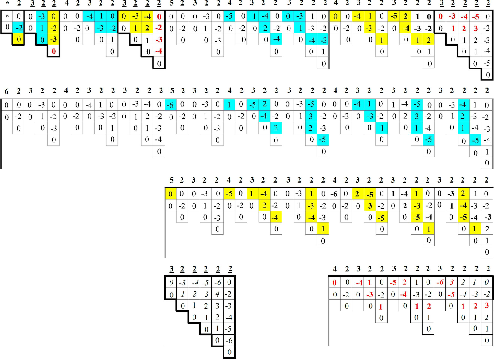
Still in Figure 3 for \(\mathcal T_7\), the first \(\tau_5^5=42\) columns (top layer) have lengths correspondingly equal to the lengths of the subsequent \(\tau_4^5=42\) columns (second layer, delimited on the right by a thick gray vertical segment). Of these, the final 28 columns have lengths correspondingly equal to the lengths of the subsequent \(\tau_3^5=28\) columns (third layer). Of these, the final 14 columns have lengths correspondingly equal to the lengths of the subsequent \(\tau_2^5=14\) columns (fourth right layer). Of these, the final 5 columns have lengths correspondingly equal to the lengths of the subsequent \(\tau_1^5=5\) columns (in the fourth left layer). It remains just \(\tau_0^5=1\) column, formed by \(k=7\) values of \(h(\alpha)\). The said numbers of columns account for the partition \(\Delta'_5=(42,42,28,14,5,1)\), representing all the columns associated with the maximal paths of \(\mathcal T_7\) formed by nodes associated with RGS’s \(\alpha\) with \(i(\alpha)=1\). Similar cases are easy to obtain in relation to \(\mathcal T_k\), for \(k<7\), where thick gray vertical segments delimit on the right the 14 (resp., 5) columns next to the first 14 (resp., 5) columns; (the same could have been done for the two columns next to the first two columns). A similar observation holds for every other row of \(\Delta'\).
Some of the heading numbers in Figure 3 appear underlined, corresponding to the final \(k-1=\tau_1^{k-2}+\tau_0^{k-2}=(k-2)+1\) columns for each exemplified \(\mathcal T_k\). The resulting column sets appear encased with a thicker border.
The subsequence \(\Phi_1\) of \(\mathcal S\), a member of a family of subsequences \(\{\Phi_j ; 1\le j\in\mathbb{Z}\}\) satisfying for \(j>1\) the rules 1–3 below, is such that \(i(\Phi_1)\) is the subsequence of \(i(\mathcal S)\) formed by all indices \(i(\alpha)\) larger than 1, exemplified in the heading line of Figure 3. The mentioned rules 1–3 are as follows:
| α | h(α) | α1 | h(α1) | α2 | h(α2) | α3 | h(α3) | α4 | h(α4) | α5 | h(α5) |
|---|---|---|---|---|---|---|---|---|---|---|---|
| 0 | * | 00 | * | 10 | 0 | ||||||
| 1 | 0 | 01 | 0 | 11 | -2 | 12 | 0 | ||||
| 0 | * | 000 | 0 | 100 | 0 | ||||||
| 1 | 0 | 001 | 0 | 101 | 0 | ||||||
| 10 | 0 | 010 | 0 | 110 | -3 | 120 | 0 | ||||
| 11 | -2 | 011 | -2 | 111 | 1 | 121 | -2 | ||||
| 12 | 0 | 012 | 0 | 112 | 0 | 122 | 1 | 123 | 0 | ||
| 0 | * | 0000 | * | 1000 | 0 | ||||||
| 1 | 0 | 0001 | 0 | 1001 | 0 | ||||||
| 10 | 0 | 0010 | 0 | 1010 | 0 | ||||||
| 11 | -2 | 0011 | -2 | 1011 | -2 | ||||||
| 12 | 0 | 0012 | 0 | 1012 | 0 | ||||||
| 100 | 0 | 0100 | 0 | 1100 | -4 | 1200 | 0 | ||||
| 101 | 0 | 0101 | 0 | 1101 | 0 | 1201 | 0 | ||||
| 110 | -3 | 0110 | -3 | 1110 | 1 | 1210 | -3 | ||||
| 111 | 1 | 0111 | 1 | 1111 | -3 | 1211 | 1 | ||||
| 112 | 0 | 0112 | 0 | 1112 | 0 | 1212 | 0 | ||||
| 120 | 0 | 0120 | 0 | 1120 | 0 | 1220 | -4 | 1230 | 0 | ||
| 121 | -2 | 0121 | -2 | 1121 | -2 | 1221 | 2 | 1231 | -2 | ||
| 122 | -3 | 0122 | -3 | 1122 | 1 | 1222 | 1 | 1232 | -3 | ||
| 123 | 0 | 0123 | 0 | 1123 | 0 | 1223 | 0 | 1233 | -4 | 1234 | 0 |
the first term of \(\Phi_j\) is \[\phi_1=\begin{cases} \mbox{the RGS }1,&\mbox{ if }j=1;\\ \mbox{the smallest RGS with suffix }(j-1)(j-1),&\mbox{ if }j>1;\\ \end{cases}\]
if \(\alpha=a_{k-1}\cdots a_1\in\Phi_j\) and either \(a_1=0\) or \(a_{k-1}\cdots a_2a'_1\notin\Phi_j\) for every \(a'_1<a_1\), then \(\alpha|j\in\Phi_j\) for \(j\in[0,a_1]\); in that case, if \(\alpha_{j'}\in\Phi_j\) with \(\alpha_{j'}=a_{k-1}\cdots a_2(a_1+j')\), for \(1\le j'\in\mathbb{Z}\), then \(\alpha_{j'}|j\in\Phi_j\);
for each maximal subsequence \(S=(\iota,2,\ldots,2)\) of \(i(\mathcal S)\) (\(\iota>2\)), if there are \(z\) penultimate terms \(i=2\) of \(S\) (\(z>0\)) heading maximal vertical prefixes of a fixed length \(y\) in \(h(\Phi_j)\) (\(y>0\)) and ending at \(h(\alpha_j)=h(a_{k-1}\cdots a_3(y+j)y)\) (\(j\in[0,z[\)), then \(\alpha_{j'}=a_{k-1}\cdots a_3(y+z)j'\in\Phi_j\), for \(j'\in]y,y+z]\), yielding a vertical suffix \(\{h(\alpha_{j'});j'\in]y,y+z]\}\).
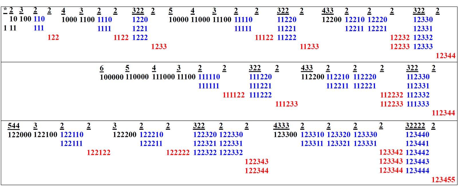
Example 8. The three rectangular enclosures of Figure 4 contain in left-to-right columnwise form (only showing those columns with yellow squares in Figure 3) the subsequence \(\Phi_1\) of \(\mathcal S\) in Subsection 6.1, (of RGS’s \(\alpha\) in yellow squares). Such enclosures contain in red the RGS’s for the prefixes in item 3 above, and in blue the RGS’s for the suffixes.
The columns in the formations of Subsection 6.2, as in Figure 3, end up with null values \(h(\alpha)=0\), which correspond to the terminal nodes \(\alpha\) of maximal paths that after their initial nodes \(\beta\) with \(i(\beta)>1\), have the remaining nodes \(\beta'\) with \(i=i(\beta')=1\). Clearly, the associated nodes \(\alpha\) have degree 1 in the pertaining trees \(\mathcal T_k\).
Theorem 6. Let \(\alpha\) be a node of \(\mathcal T_k\). Then,
if \(\alpha\) is a terminal node of a maximal path of \(\mathcal T_k\) whose initial node \(\beta\) has \(i(\beta)>1\) and whose remaining nodes \(\gamma\) have \(i(\gamma)=1\), then \(g(\alpha)=0\);
if \(\alpha=a_{k-1}\cdots a_1\) with \(a_{k-1}=1\) and \(a_j=0\), for \(j=1,\ldots, k-2\), then \(g(\alpha)=0\).
Proof. Item 1 in the statement arises because of the presence of the substring \(1'1''\) in \(F(\alpha)\). Item 2 arises because of the presence of all substrings \(j'j''\) in \(F(\alpha)\), for \(j=1,\ldots,k-1\). ◻
Theorem 7. Let \(\alpha_1\) be a node of \(\mathcal T_k\). Then, \(\alpha'_1=1|\alpha_1\) is a node of \(\mathcal T_{k+1}\) and
if \(h(\alpha_1)\in\Phi_1\), then \(h(\alpha'_1)\in\Phi_1\) and \(h(\alpha'_1)=k-h(\alpha_1)\);
if \(h(\alpha_1)\notin\Phi_1\), then \(h(\alpha'_1)\notin\Phi_1\) and \(h(\alpha'_1)=h(\alpha_1)\).
Proof. Item 1 in the statement occurs exactly when the substring \(k'k''\) in \(F(\alpha)\) changes position from one side of \(1'\) to the opposite side in the procedure of Theorem 1 starting at the parent \(\beta\) of \(\alpha\) and ending at \(\alpha\). Item 2 occurs exactly when that is not the case. ◻
Example 9. Since \(\alpha_1=1\) is a node of \(\mathcal T_2\) as in Theorem 6 item 1, then \(\alpha'_1=1|\alpha_1=11\) is a node of \(\mathcal T_3\) with \(h(\alpha'_1)=h(11)=h(1)-k=0-2=-2\in\Phi_1\), by Theorem 7 item 1. This is indicated by \(h(1)=0\) in the upper leftmost yellow square in Figure 3 and its accompanying \(h(11)=-2\) as the upper leftmost red integer in the figure. Note that this pattern is continued by associating each yellow square in Figure 3 to a corresponding red integer for all \(k<7\). We can annotate this via the successive pairs \((\alpha_1,h(\alpha_1))\) taken by reading the data in Figure 3 from left to right and from top downward: \[^{(1(0),11(-2)), (10(0),110(-3)), 11(-2),111(1)),(100(0),1100(-4)),(110(-3),1110(1)),(111(1),1111(-3)),(122(-3),1122(1)).}\]
The last pair here arises from \(h(122)=-3\), which follows from Corollary 3, below.
Theorem 8. Let \(1<j\le k\in\mathbb{Z}\). Let \(\alpha_j=1\cdots(j-1)(j-1)a_{k-j-1}\cdots a_1\) be a node of \(\mathcal T_k\). Then, \(\alpha'_j=1\cdots (j-1)ja_{k-j-1}\cdots a_1\) is a node of \(\mathcal T_k\) and
if \(h(\alpha_j)\in\Phi_j\), then \(h(\alpha'_j)=k-h(\alpha_j)\);
if \(h(\alpha_j)\notin\Phi_j\), then \(h(\alpha'_j)=h(\alpha_j)\).
Proof. Similar to the proof of Theorem 7. ◻
Corollary 3. Let \(1\le k\in\mathbb{Z}\). Let \(\alpha_2=11a_{k-3}\cdots a_1\) be a node in \(\mathcal T_k\). Then, \(\alpha'_2=12a_{k-3}\cdots a_1\) is a node of \(\mathcal T_k\) and
if \(h(\alpha_2)\in\Phi_2\), then \(h(\alpha'_2)=k-h(\alpha_2)\);
if \(h(\alpha_2)\notin\Phi_2\), then \(h(\alpha'_2)=h(\alpha_2)\).
Example 10. Applying Corollary 3 to \(\alpha_2=11,110,111,112\), with respective \(h(\alpha_2)=-2,-3,1,0\in\Phi_2\) yields \(\alpha'_2=12,120,121,122\) with respective \(h(\alpha'_2)=0,0,-2,-3\). In Figure 5, the RGS’s \(\alpha_2\) are shown in light-blue squares while the corresponding RGS’s \(\alpha'_2\) are shown in yellow squares. Figure 5 extends this coloring for \(k\le 7\).
Corollary 4. Let \(1\le k\in\mathbb{Z}\). Let \(\alpha_3=122a_{k-4}\cdots a_1\) be a node of \(\mathcal T_k\). Then, \(\alpha'_3=123a_{k-4}\cdots a_1\) is a node of \(\mathcal T_k\) and
if \(h(\alpha_3)\in\Phi_3\), then \(h(\alpha'_3)=k-h(\alpha_3)\);
if \(h(\alpha_3)\notin\Phi_3\), then \(h(\alpha'_3)=h(\alpha_3)\).
Example 11. Applying Corollary 4 to \(\alpha_3=122,1220,1221,1222,1223\) with respective \(h(\alpha_3)=-3,-4,2,1,0\in\Phi_3\) yields \(\alpha'_3=123,1230,1231,1232,1233\) with respective \(h(\alpha'_3)=0,0,-2,-3,-4\). In Figure 5, the RGS’s \(\alpha_3\) are shown in thick black while the corresponding RGS’s \(\alpha'_3\) are shown in thick red. Moreover, Figure 5 extends this font treatment for \(k\le 7\). For \(k=7\), numbers in Italics in Figure 5 corresponds to members of \(\Phi_4\).
Both the integer-valued functions \(i=i(\alpha)\) of Theorem 1 and \(h=h(\alpha)\) of display (4) have the same domain, \({\mathcal S}\!\setminus\!\beta(0)\). A partition of a string \(A\) is a sequence of substrings \(A_1,A_2,\ldots,A_n\) whose concatenation \(A_1|A_2|\cdots|A_n\) is equal to \(A\).
Theorem 9. The following items hold.
(A) The node set of \(\mathcal T_{k+1}\) is given by the string \(A_k^k=A_1^1|A_2^2|\cdots |A_{k-1}^{k-1}|\) \(A_{k-1}^k\), with partition \(\{A_1^1,A_2^2,\ldots,A_{k-1}^{k-1},A_{k-1}^k\}\), each \(A_i^j\) as a column set as in Table 2 and Figures 3–5, refined by splitting the last column \(A_{k-2}^k\) of \(A_{k-1}^k\) into the set \(B_{k-2}^k\) of its first \(k-1\) entries and the set \(C_{k-2}^k\) of its last entry, \(a_{k-1}a_{k-2}\cdots a_1=12\cdots (k-1)\). The sizes \(|A_1^1|\), \(|A_2^2|\), \(\ldots\), \(|A_{k-1}^{k-1}|\), \(|B_{k-2}^k|\), \(|C_{k-2}^k|\) form the line \(\Delta'_{k-1}\) of \(\Delta'\).
(B) The sequence \(h({\mathcal S}\!\setminus\!\beta(0))\) is generated by stepwise consideration of the trees \(\mathcal T_{k+1}\), (\(1\le k\in\mathbb{Z}\)). In the \(k\)-th step, the determinations in Theorems 7 and 8 are to be performed in the natural order of the \((k+1)\)-germs \(\alpha_j\). More specifically, the \(k\)-step completes those determinations, namely \((\alpha_j,h(\alpha_j))\rightarrow(\alpha'_j,h(\alpha'_j))\), for the lines of \(\Delta'\) corresponding to the sets \(A_j^j\) (\(j=1,\ldots,k-1\)), and ends up with the determinations \((\alpha_k,h(\alpha_k))\rightarrow(\alpha'_k,h(\alpha'_k))\) in the line corresponding to \(B_{k-2}^k\) and \((\alpha_{k+1},h(\alpha_{k+1}))\rightarrow(\alpha'_{k+1},h(\alpha'_{k+1}))\) in the final line, corresponding to \(C_{k-2}^k\).
Proof. Item (A) represents the set of nodes of \(\mathcal T_{k+1}\) via \(A_k^k\) and \(\Delta'_{k-1}\). This is used in item (B) to express the stepwise nature of the generation of the sequence \(h({\mathcal S}\!\setminus\!\beta(0))\). The methodology in the statement is obtained by integrating steps applying Theorems 7 and 8 in the way prescribed, that yields the correspondence with the lines of \(\Delta'\). ◻
Example 12. Theorem 9 is exemplified via Table 5, where the lists corresponding to \(\mathcal T_2\), \(\mathcal T_3\) and \(\mathcal T_4\) are represented according to the respective pairs \((\alpha,h(\alpha))\) indicating column pairs \((\alpha,h(\alpha))\) and \((\alpha_j,h(\alpha_j))\), for \(j=1,2,3,4,5\), as shown in the heading line of the table.
The first pair, \((\alpha,h(\alpha))\) shows RGS’s \(\alpha\) in each case and their corresponding \(h(\alpha)\). The following pair, \((\alpha_1,h(\alpha_1))\), shows the \(k\)-germs \(\alpha_1\) corresponding to the RGS’s \(\alpha\) of the first column and \(h(\alpha_1)=h(\alpha)\) but in bold trace if corresponding to a yellow square as in Figure 3; in that case, the subsequent determinations \((\alpha_1,h(\alpha_1))\rightarrow(\alpha'_1,h(\alpha'_1))\) have the corresponding \(h(\alpha'_1)\) in Italics. This is the case of \(h(01)=0\) in bold trace and \(h(11)=-2\) in Italics, that we may indicate “\(h(01)=0\rightarrow_1(11)=-2\)”. If a determination \((\alpha_2,h(\alpha_2))\rightarrow(\alpha'_2,h(\alpha'_2))\) happens, then the numbers in Italics are assigned on their right to numbers in bold trace, again. The cases with bold trace and Italics in Table 5 can then be summarized as follows: \[\begin{array}{ll} {h(01)=0\rightarrow_1h(11)=-2\rightarrow_2h(12)=0,}&{h(011)=-2\rightarrow_1h(111)=1\rightarrow_2h(121)=-2,}\\ {h(010)=0\rightarrow_1h(110)=-3\rightarrow_2h(120)=0,}& {h(1000)=0\rightarrow_1h(1100)=-4\rightarrow_2h(1200)=0,}\\ {h(0110)=-3\rightarrow_1h(1110)=1\rightarrow_2h(1210)=-3,}&{h(1121)=-2\rightarrow_2h(1221)=2\rightarrow_3h(1231)=-2,}\\ {h(0111)=1\rightarrow_1h(1111)=-3\rightarrow_2h(1211)=1,}& {h(0122)=-3\rightarrow_1h(1122)=1\rightarrow_2h1222)=1\rightarrow_3h(1232)=-3,}\\ {h(1223)=0\rightarrow_3h(1233)=-4\rightarrow_4h(1234)=0.}&\end{array}\]
Corollary 5. The sequence of pairs \((a(S\!\setminus\!\beta(0)),h(S\!\setminus\!\beta(0)))\) allows to retrieve any vertex \(v\) in \(O_k\) (resp., \(M_k\)) by locating its oriented \(n\)– (resp., \(2n\)-) cycle in the cycle-factor of [4,5] or in the \(\mathbb{Z}_n\)– (resp., \(\mathbb{D}_n\)-) classes as in Section 1, and then locating \(v\) departing from the anchored Dyck word in such cycle or class; the sequence also allows to enlist all such vertices \(v\) by ordering their cycles (resp., classes), including all vertices in each such cycle (resp., class), starting with the corresponding anchored Dyck word.
Proof. The function \(a(S\!\setminus\!b(0))\), arising from Theorem 1, yields the required update locations, while the function \(h({\mathcal S}\!\setminus\!\beta(0))\) yields the specific updates, as determined in Theorem 9. This produces the corresponding signatures. Then, Theorem 3 allows to recover the original Dyck words from those signatures, and thus the vertices of \(O_k\) (resp., \(M_k\)) by local translation in their containing cycles in the mentioned cycle-factors, or cyclic (resp., dihedral) classes. ◻
It is known that asymptotically the Catalan numbers \(C_k\) grow as \(\frac{4^k}{k^{\frac{3}{2}}\sqrt{\pi}}\), which is the limit of the single-update process that takes to the determination of all Dyck words of length \(n=2k+1\), as \(k\) tends to infinity. By Corollary 5, an orderly determination of all the vertices of \(O_k\), resp., \(M_k\), is then asymptotically \(\frac{4^k}{k^{\frac{3}{2}}\sqrt{\pi}}(2k+1)\), resp., \(\frac{4^k}{k^{\frac{3}{2}}\sqrt{\pi}}(4k+2)\).