
The intersection of graph theory and linear algebra revolves primarily around the adjacency matrix , a fundamental representation that encapsulates the structural essence of a graph in mathematical terms. In the 1950s, mathematicians confronted the challenge of melding the robust frameworks of matrices with the intricate structures of graphs, giving rise to a novel approach in mathematical inquiry. A pivotal concept that emerged was the exploration of eigenvalues within this context. For graphs, the eigenvalues of the adjacency matrix hold profound significance, as they directly mirror the eigenvalues of the graph itself. This collective set of eigenvalues constitutes the spectrum of the graph, a crucial descriptor that transcends the graph’s visual depiction and encapsulates its intrinsic properties in a numerical form. Over the years, the study of graph spectra has flourished, finding wide-ranging applications across disciplines such as theoretical chemistry, quantum mechanics, statistical physics, and computer science. In each domain, the spectrum of a graph provides essential insights and tools for understanding complex networks, predicting behavior in physical systems, optimizing algorithms, and much more. Thus, from its theoretical origins to its practical applications, the interplay between graph theory and linear algebra through the lens of adjacency matrices and eigenvalues continues to enrich both mathematical theory and real-world problem-solving [2].
In the exploration of network theory, N. Alon introduced a significant concept known as the extended double cover (EDC) of a graph, aimed at leveraging magnifiers to generate expanders. Building on this foundation, Z. Chen’s work in [1] concentrated on the spectral characteristics of the EDC, sparking further interest and investigation. Inspired by this research, our focus shifted towards defining the extended \(H\)-cover of a graph, denoted as \(G^*_H\), where this construction aligns with the EDC when \(H\) corresponds to the complete graph \(K_2\).
Graph theory has gained significant attention due to its applications in network analysis and complex systems. The study of novel resolvability parameters continues to grow [3], alongside the exploration of mixed metric dimensions in specialized networks [4]. Researchers have also investigated fuzzy graph models for practical challenges like human trafficking [5], and nanotube structures [6]. New parameters have been applied in biochemical modeling as well [7]. Recently, the concept of mixed partition dimension has added to the depth of graph resolvability studies [8]. Labeling techniques such as cycle-super magic labeling have introduced innovative ways to represent complex chains [9]. Moreover, the need for robust systems has led to studies on fault-tolerant identification in graphs [10]. Earlier work on eccentric connectivity indices also laid the foundation for chemical graph modeling [11].
In our study, we focus on simple, connected, and undirected graphs, fundamental structures in graph theory. Basic terminologies from graph theory are essential for our discussions, as outlined in references [12, 13]. The degree of a vertex \(v\), denoted as \(deg(v)\), represents the number of vertices adjacent to \(v\). The maximum degree of a graph \(G\) is denoted as \(\Delta\), while its minimum degree is denoted as \(\delta\). A vertex with degree one is termed a pendant vertex, and a vertex that is adjacent to every other vertex in \(G\) is known as a universal vertex. The neighbors of a vertex \(v\), denoted as \(N(v)\), comprise the set of all vertices adjacent to \(v\). The complement of a graph \(G\), denoted \(\overline{G}\), shares the same vertex set as \(G\), with edges between vertices that are not adjacent in \(G\). The chromatic number of a graph \(G\), denoted \(\chi(G)\), signifies the minimum number of colors required to color all vertices such that no two adjacent vertices share the same color.
The shortest path between any two vertices \(u\) and \(v\) in a graph \(G\) is termed the \(u-v\) geodesic, representing the minimal sequence of edges connecting them. The eccentricity of a vertex \(u\) is defined as the maximum distance from \(u\) to any other vertex in the graph, capturing its ’reach’ within the network. The maximum eccentricity among all vertices defines the diameter of the graph, while the minimum eccentricity determines its radius, representing the extent of the graph’s spread from its most distant to its closest vertex. For any pair of vertices \(u\) and \(v\), the set \(I[u,v]\) encompasses all vertices that lie on any \(u-v\) geodesic, including \(u\) and \(v\) themselves. Extending this concept to a subset \(S\) of vertices in \(G\), the set \(I[S]\) encompasses all vertices that lie on the geodesics between every possible pair of vertices in \(S\), encompassing both the vertices within \(S\) and those connecting them through shortest paths.
The discussion in the subsequent sections are based on the following definitions.
Definition 1. [12] The join of graphs \(G\) and \(H\) is denoted as \(G\lor H\). It consists of the vertex set \(V(G) \cup V(H)\), where each vertex of \(G\) is adjacent to all vertices of \(H\) and vice-versa.
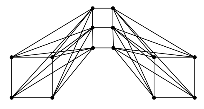
Definition 2. [14] The Indu-Bala product of graphs \(G\) and \(H\) is denoted as \(G\blacktriangledown H\). It consists of two copies of \(G\lor H\), where there is an adjacency between the corresponding vertices of \(H\).
The Figure 1 represents the Indu-Bala product of paths \(C_{4}\) and \(P_{3}\).
For any graphs \(G\) and \(H\), \(\gamma_{I}(G\blacktriangledown H)=8.\)
Definition 3. [15, 16] A vertex subset \(D\) of a graph \(G=(V,E)\) is said to be a dominating set if all vertices in \(G\) are either in \(D\) or adjacent to at least one vertex in \(D\). The minimum cardinality of such a set is the domination number, denoted by \(\gamma(G)\).
Definition 4. [17] A dominating set \(D\) of a graph \(G\) is said to be a global dominating set if \(D\) is also a dominating set of \(\overline{G}\). The minimum cardinality of such a set is the global domination number denoted by \(\gamma_{g}(G)\).
Definition 5. [18] A dominating set \(D\) of a graph \(G=(V,E)\) is said to be a restrained dominating set if \(<V-D>\) has no isolated vertex. The minimum cardinality of such a set is the restrained domination number, denoted as \(\gamma_{r}(G)\).
Definition 6. [19] A dominating set \(D\) of a graph \(G=(V,E)\) is said to be a total dominating set if \(<D>\) has no isolated vertex. The minimum cardinality of such a set is the total domination number, denoted as \(\gamma_{t}(G)\).
Definition 7. [20] For a graph \(G=(V,E)\), a function \(f:V \rightarrow \lbrace 0,1,2\rbrace\) is said to be a Roman dominating function if every vertex \(v\in V\) with \(f(v)=2\) must be adjacent to at least one vertex say \(w\) such that \(f(w)=0\). The weight of a Roman dominating function is \(\sum_{v\in V} f(v)\) and the minimum among such weights is the Roman domination number, denoted as \(\gamma_{R}(G)\).
Definition 8. [21] The Italian dominating function on a graph \(G=(V,E)\) is a function \(f: V(G)\rightarrow \lbrace 0,1,2\rbrace\) which satisfies the condition that for all vertices \(v\in V(G)\) with \(f(v)=0\), \(\sum_{u\in N(v)} f(u)\geq 2\). The Italian domination number is the minimum weight of the Italian dominating function, denoted as \(\gamma_{I}(G)\).
Definition 9. [22, 23] A vertex subset \(S\) of a graph \(G=(V,E)\) is said to be a geodetic set if \(I[S]=V(G)\). The minimum cardinality of such a set is the geodetic number, denoted by \(g(G)\).
Definition 10. [24] A geodetic set \(S\) of a graph \(G=(V,E)\) is said to be a restrained geodetic set if \(<V-S>\) has no isolated vertex. The minimum cardinality of such a set is the restrained geodetic number, denoted as \(g_{r}(G)\).
Definition 11. [25] A geodetic set \(S\) of a graph \(G=(V,E)\) is said to be a total geodetic set if \(<S>\) has no isolated vertex. The minimum cardinality of such a set is the total geodetic number, denoted as \(g_{t}(G)\).
Definition 12. A geodetic set \(S\) of a graph \(G=(V,E)\) is said to be an independent geodetic set if \(S\) is an independent set. The minimum cardinality of such a set is the independent geodetic number, denoted as \(g_{i}(G)\).
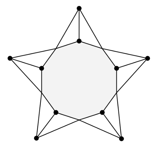
Definition 13. [26] Let \(G\) be a \((p,q)\) graph. Corresponding to every edge \(e\) of \(G\) introduce a vertex and make it adjacent with all the vertices not incident with \(e\) in \(G\). Delete the edges of \(G\) only. The resulting graph is called the partial complement of the subdivision graph(PCSD) of \(G\) denoted by \(\overline{S}(G)\).
The Figure 2 illustrates the \(PCSD\) of \(C_5\)
Theorem 1. [15, 22, 23]Let \(G\) be a graph of order \(n\) and having diameter \(d\). Then,
\(\lceil \frac{d+1}{3}\rceil \leq \gamma(G),\)
\(2\leq \min \lbrace g(G),\gamma(G)\rbrace\leq n,\)
\(g(G)\leq n-d+1\).
Theorem 2. [27]Let \(G\) and \(H\) be graphs of order \(m\) and \(n\) respectively. Then, \[\gamma(G\blacktriangledown H)= \left\{ \begin{array} [c]{l}% 2 ;\\ 2 ;\\ 4; \end{array}% \begin{array} [c]{l}% \Delta(G)=m-1 \;and\; \Delta(H)=n-1,\\ \Delta(G)=m-1 \; or\; \Delta(H)=n-1,\\ \Delta(G)\neq m-1 \; and \; \Delta(H)\neq n-1. \end{array} \right.\]
Theorem 3. For any graph \(G\), \(\gamma(G)\leq \gamma_{R}(G)\leq 2\gamma(G)\).
Theorem 4. [28] For any graphs \(G\) and \(H\), \(\chi(G\square H)=\max \lbrace \chi(G),\chi(H)\rbrace\). where \(G\square H\) denotes the cartesian product of \(G\) and \(H\).
Lemma 1. [29]Let \(G\) be a graph with an adjacency matrix \(A\) and \(spec(G) =\{ \lambda_1,\lambda_2,…,\lambda_p\}\), Then, \(det A = \prod\limits_{i=1}^p {\lambda_i}\). Also for any polynomial \(P(x)\), \(P(\lambda)\) is an eigenvalue of \(P(A)\) and hence \(det P(A) =\prod\limits_{i=1}^p {P(\lambda_i)}\).
Lemma 2. [29]Let \(A\) and \(B\) be two matrices and \(F= A\otimes B\) be their tensor product.Then, \(spec(F)= \{ \lambda _i\mu_j | \lambda_i \in spec(A),\mu_j \in spec(B)\}\).In particular let \(G\) and \(H\) be two graphs of order \(p\) and \(p^{\prime}\) respectively with \(spec(G) = \{\lambda_i\}, i = 1\) to \(p\) and \(spec(H) = \{\mu_j\}, j = 1\) to \(p^{\prime}\). Let \(F= G\otimes H\), the tensor product of \(G\) and \(H\). Then, \(spec(F)=\{\lambda_i\mu_j\}, i = 1\) to \(p\) and \(j= 1\) to \(p^{\prime}\)
Lemma 3. [29]Let \(G\) be a connected regular graph of degree \(r -\) with \(spec(G) =\{ r=\lambda_1, \lambda_2,…,\lambda_p\}\). Let \(\tau (G)\) denote the number of spanning trees of \(G\). Then \[\tau (G)= \frac{1}{p} \prod\limits_{i=2}^p (r – \lambda_i) =\frac{1}{p} P^{\prime} (G,r),\] where \(P^{\prime}\) denote the derivative of the characteristic polynomial of \(G\).
Lemma 4. [30]\[\mathcal{E}(C_p) = \begin{cases} 4\cot \frac{\pi}{p}~ ;~~p\equiv 0(mod~4),\\ 2\cot \frac{\pi}{2p}\cos \frac{\pi}{2p}~ ;~~p\equiv 1(mod~4),\\ 4\csc \frac{\pi}{p}~ ;~~p\equiv 2(mod~4),\\ 2\cot \frac{\pi}{2p}\sec \frac{\pi}{2p}~;~~p\equiv 3(mod~4).\\ \end{cases}\]
In this section, we introduce the extended \(H-\) cover of \(G\), denoted as \(G^*_H\) and study its spectrum and energy. Also, the number of spanning trees in \(G^*_H\) is determined.
Definition 14. Let \(G = (V,E)\) be a simple undirected graph with \(p\) vertices \(\{v_1,v_2,…,v_p\}\) and an adjacency matrix \(A\). Let \(H\) be a graph on \(n\) vertices \(\{u_1,u_2,…,u_n\}\). The extended \(H-\) cover of \(G\), \(G^*_H\) is defined as a graph with vertex set \(\{U_1,U_2,…,U_n\}\) where \(U_i=\{v_1^i,v_2^i,…,v_p^i\}\) in which adjacency is with vertices of \(U_i\) and \(U_j\) only whenever \(u_i\) adjacent to \(u_j\) in \(H\). The adjacency is defined as follows.
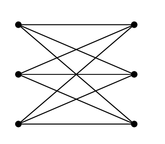
Let \(v_a^i \in U_i\) and \(v_b^j \in U_j\) . Then \(v_a^i\) is adjacent to \(v_b^j\) if and only if \(a=b\) or \(v_a\) adjacent to \(v_b\) in \(G\). For example the complete \(r-\) partite graph \(K_{p,p,…,p}\) on \(pn\) vertices is the extended \(K_r\) cover of \(K_p\). It is easy to observe that \(G^*_H\) is connected if and only if both \(G\) and \(H\) are connected. Also \(G^*_H\) is regular if and only if \(G\) and \(H\) are regular. If \(G\) is \(r-\) regular and \(H\) is \(t-\) regular then \(G^*_H\) is \(t(r+1) -\) regular. Figure 3 illustrates this with \(G=C_{3}\) and \(H=P_{2}.\)
Theorem 5. Let \(G\) and \(H\) be two graphs with \(spec(G) = \{ \lambda_1, \lambda_2,…,\lambda_p\}\) and \(spec(H) = \{\mu_1,\mu_2…,\mu_n\}\)respectively. Then \(spec(G^*_H) =\{ \mu_j (\lambda_i+1)\},i = 1\) to \(p\) and \(j=1\) to \(n\).
Proof. Let \(A\) and \(B\) respectively denote the adjacency matrices of \(G\) and \(H\). Then by the definition of \(G^*_H\), its adjacency matrix can be written as \(B\otimes (A+I)\) and hence the theorem follows from Lemma 1 and 2.
For instance, consider the complete \(n\)-partite graph \(K_{p,p,\ldots,p}\), which can be denoted as \((K_p)^*_{K_n}\). Given that the spectrum of \(K_p\) is
\[\left( \begin{array}{cc} p-1 & -1 \\ 1 & p-1 \\ \end{array} \right),\] by Theorem 5, the spectrum of \(K_{p,p,\ldots,p}\) is
\[\left( \begin{array}{ccc} p(n-1) & -p & 0 \\ 1 & n-1 & n(p-1) \\ \end{array} \right).\] ◻
Corollary 1. \[\mathcal{E}(K_p)^*_{H}=p~ \mathcal{E}(H).\]
Proof. We have spectrum of \(K_p = \left( {\begin{array}{*{20}c} {p-1} & { – 1} \\ {1} & {p-1} \\ \end{array} } \right)\). Therefore by Theorem 5, \(spec (K_p)^*_{H} =\{ \mu_j p,0\}\), \(j=1\) to \(n\) and \(0\) with multiplicity \(n(p-1)\).
Therefore \(\mathcal{E}(K_p)^*_{H}= p \sum_{1}^{n} \mid {\mu_j}\mid = p~ \mathcal{E}(H)\) ◻
Corollary 2. If \(H_1\) and \(H_2\) are equienergetic, then \((K_p)^*_{H_1}\) and \((K_p)^*_{H_2}\) are equienergetic.
Proof. By Corollary 1, \(\mathcal{E}(K_p)^*_{H}=p~ \mathcal{E}(H)\). Since \(H_1\) and \(H_2\) are equienergetic, \(\mathcal{E}(H_1) = \mathcal{E}(H_2)\)\(.~ Therefore ~\)\(\mathcal{E}(K_p)^*_{H_1} = p~ \mathcal{E}(H_1) = p~ \mathcal{E}(H_2) = \mathcal{E}(K_p)^*_{H_2}\) ◻
Corollary 3. If \(H_1\) and \(H_2\) are equienergetic, then \((K_{p,p})^*_{H_1}\) and \((K_{p,p})^*_{H_2}\) are equienergetic.
Proof. We have spectrum of \(K_{p,p} = \left( {\begin{array}{*{20}c} {p} & { – p} & {0} \\ {1} & {1} & {2p-2} \\ \end{array} } \right)\). If \(spec(H) = \{\mu_1,\mu_2…,\mu_n\}\), then by Theorem 5, \(spec (K_{p,p})^*_{H} =\{\mu_j (p+1), \mu_j (-p+1), \mu_j (0+1)\}\) and \(j=1\) to \(n\).
\[\mathcal{E} (K_{p,p} )^*_{H}= \{ (p+1)\mathcal{E}(H)+ (p-1)\mathcal{E}(H) + \mathcal{E}(H)\} = (2p+1)\mathcal{E}(H).\]
Since \(H_1\) and \(H_2\) are equienergetic, \(\mathcal{E}(H_1) = \mathcal{E}(H_2)\).
Therefore \[\mathcal{E}(K_{p,p})^*_{H_1} = (2p+1)~ \mathcal{E}(H_1) = (2p+1)~ \mathcal{E}(H_2) = \mathcal{E}(K_{p,p})^*_{H_2}.\] ◻
Corollary 4. If \(G_1\) and \(G_2\) are cospectral then \((G_1)^*_{H}\) and \((G_2)^*_{H}\) are cospectral.
Corollary 5. If \(H_1\) and \(H_2\) are cospectral then \(G^*_{H_1}\) and \(G^*_{H_2}\) are cospectral.
Remark 1. By setting any two of the above graphs as \(G_1\) and \(G_2\), we can generate \(4\) cospectral graphs. Repeating this procedure will give arise to an infinite family of cospectral graphs.
Theorem 6. Let \(G\) and \(H\) be two connected regular graphs with regularity \(r-\) and \(t-\) respectively. Let \(spec(G) = \{ r = \lambda_1,\lambda_2,…,\lambda_p\}\) and \(spec(H) = \{ t = \mu_1,\mu_2,…,\mu_n\}\). Then
\[\tau(G^*_H) = t^{p-1}(r+1)^{n-1} \tau(G)\tau(H)\prod\limits_{j=2}^n \prod\limits_{i=2}^p (t(r+1) – \mu_j(\lambda_i+1)).\]
Proof. From the given conditions we can see that \((G^*_H)\) is \(t(r+1) -\) regular and is connected. By Theorem 5 we get the spectrum of \(G^*_H\). Then by Lemma 3 we have
\[\begin{aligned}\tau(G^*_H) =& \frac{1}{np}\prod\limits_{{i=1}, {j=1} ~\&{i,j}\neq1}^{{p},{n}}[t(r+1) – \mu_j(\lambda_i+1)]\\ =&\frac{1}{np}\prod\limits_{i=2}^p(t(r-\lambda_i))\prod\limits_{j=2}^n((r+1)(t-\mu_j))\prod\limits_{j=2}^n\prod\limits_{i=2}^p(t(r+1)-\mu_j(\lambda_i+1))\\ =&t^{p-1}(r+1)^{n-1}\tau(G)\tau(H)\prod\limits_{j=2}^n \prod\limits_{i=2}^p (t(r+1) – \mu_j(\lambda_i+1)).\end{aligned}\] ◻
Using the above theorem, we can determine the number of spanning trees of \(G^*_H\) from the spectra of \(G\) and \(H\). However, sometimes computing the actual spectra of these graphs is not straightforward, even if we have determined their characteristic polynomials. The following corollary assists in finding the number of spanning trees of \(G^*_H\) using the characteristic polynomial of \(G\) and the spectrum of \(H\).
Corollary 6. Let \(G\) and \(H\) be two connected regular graphs with regularity \(r-\) and \(t-\) respectively. Let \(spec(H) = \{t=\mu_1,\mu_2,…,\mu_n\}\). Then
\[\tau(G^*_H)= \dfrac{1}{npt} P^{\prime}(G,r)\prod\limits_{j=2}^n P(G, \dfrac{t(r+1)-\mu_j}{\mu_j}),\] where \(P\) is the characteristic polynomial and \(P^{\prime}\) its derivative.
Proof. By Lemma 3, we have \(\tau(G^*_H)=\dfrac{1}{np}P^{\prime}(G^*_H, t(r+1))\). Then the corollary follows from the fact that the characteristic polynomial of \((G^*_H)\) is \(\prod\limits_{j=1}^n P(G, \dfrac{x- \mu_j}{\mu_j})\) where \(P(G,x)\) is that of \(G\). ◻
Theorem 7. Let \(G\) be an \(r-\) regular graph and \(H\) be any graph. Then, \[\mathcal{E}( {\overline G}^{*}_H)=\mathcal{E}(H)(\mathcal{E}\bar(G)+p-2r).\]
Proof. Let \(G\) be an \(r-\) regular graph with \(spec(G) = \{r=\lambda_1,\lambda_2,…,\lambda_p\}\). Since \(G\) is regular, the spectrum of its complement \(\overline {G}\) is \(spec(\overline{G}) =\{ p-r-1,-1 -\lambda_2,…,-1-\lambda_p\}\). Let \(H\) be any graph with \(spec(H)=\{\mu_1,\mu_2,…,\mu_n\}\). Then by Theorem 5, we have \[\begin{aligned} spec~ ({\overline G}^*_H) &=\{\mu_j(-\lambda_i)\}\bigcup \{\mu_j(p- r)\},i = 2\text{ to }p \text{ and }j=1-n\\ &=\{-\mu_j.~ spec(G), -\mu_j.~(p- r)\} – \{-\mu_j.r\}. \end{aligned}\]
Thus \[\begin{aligned} \mathcal{E}({\overline G}^{ *}_H)=&\sum_{{i=1} ~ to~ {p},~{j=1} ~ to~ {n}}\mid {\lambda_i\mu_j} \mid +(p-r) \sum_{1}^{n} \mid {\mu_j}\mid – r \sum_{1}^{n} \mid {\mu_j}\mid \\ =&\sum_{{i=1} ~ to~ {p},~{j=1} ~ to~ {n}} \mid {\lambda_i\mu_j} \mid +(p-r) \sum_{1}^{n} \mid {\mu_j}\mid – r ~\mathcal{E}(H) \\ =& \mathcal{E}(G)\mathcal{E}(H)+ (p-2r) \mathcal{E}(H)\\ =&\mathcal{E}(H)[{\mathcal{E}(G) + p-2r}]. \end{aligned}\] ◻
Corollary 7. \[\mathcal{E}(({\overline C_p})^{*}_H)=\mathcal{E}(H)(\mathcal{E}(C_p)+p-4).\]
Corollary 8. If \(G_1\) and \(G_2\) are two \(r-\)regular equienergetic graphs then \(({\overline G_1}^{*})_H\) and \(( {\overline G_2}^{*})_H\) are equienergetic.
Corollary 9. If \(H_1\) and \(H_2\) are equienergetic then \(({\overline G}^{*})_{H_{1}}\) and \(( {\overline G}^{*})_{H_{2}}\) are equienergetic where \(G\) is any \(r-\) regular graph.
Theorem 8. Let \(G = C_p \times K_2.\) Then \[\mathcal{E}(G^*_H)= \mathcal{E}(H)(2p+\mathcal{E}(C_p)).\]
Proof. Let the \(spec(C_p) =\{\lambda_1,\lambda_2,…,\lambda_p\}\). Then from [29], \(spec(C_p\times K_2)= \lbrace\lambda_i\pm 1\rbrace\),\(i=1\) to \(p\). Hence from Theorem 5 it follows that \(spec(G^*_H)= \lbrace\mu_j(\lambda_i+2),\mu_j\lambda_i\rbrace\),\(i=1\) to \(p\) and \(j=1\) to \(n\) where \(\lambda_i \in spec(C_p)\) and \(\mu_j \in spec(H)\). Thus
\[\begin{aligned} \mathcal{E}(G^*_H) =& (\sum_{j =1}^{n} \mid {\mu_j}\mid )(\sum_{i =1}^{p} \mid {\lambda_i+2}\mid ) +\sum_{j =1}^{n} \mid {\mu_j}\mid \sum_{i =1}^{p} \mid {\lambda_i}\mid \\ =& 2p \mathcal{E}(H) +\mathcal{E}(C_p)\mathcal{E}(H). \end{aligned}\]
The expression for \(\mathcal{E}(G^*_H)\), then follows from Lemma 4. ◻
Different graph parameters of the Indu-Bala product of graphs were discussed in [27, 31, 32]. In this section, we are discussing the chromatic number and some domination variants of Indu-Bala product of graphs. From the definition of Indu-Bala product of two graphs \(G\) and \(H\), we can consider \(G\blacktriangledown H\) as first taking \(H\square K_{2}\) and then taking the join of each copy of \(H\) in \(H\square K_{2}\) with \(G\).
Theorem 9. Let \(G\) and \(H\) be any two connected graphs. Then, \[\chi(G\blacktriangledown H)= \chi(G)+\chi(H).\]
Proof. By definition, \(G \blacktriangledown H\) consists of two copies of \(G + H\). According to Theorem 4, the two copies of \(H\) in \(G \blacktriangledown H\) can be colored using \(\chi(H)\) colors. However, none of these colors can be assigned to any vertices in the two copies of \(G\) within \(G \blacktriangledown H\). Additionally, there is no adjacency between the corresponding vertices of the two copies of \(G\). Therefore, in \(G \blacktriangledown H\), the two copies of \(G\) can be colored using \(\chi(G)\) colors. Consequently \(\chi(G\blacktriangledown H)= \chi(G)+\chi(H)\). ◻
Corollary 10. Let \(G\) and \(H\) be the graphs of order \(m\) and \(n\) \((m,n>1)\) respectively. Then, \(\chi(G\blacktriangledown H)=m+n\) if and only if \(G\cong K_{m}\) and \(H\cong K_{n}\).
Proof. Let \(\chi(G \blacktriangledown H) = m + n\), and assume that either \(G\) or \(H\) is not a complete graph. Without loss of generality, let’s assume \(G\) is not complete. Then, \(\chi(G) < m\), and in \(G \blacktriangledown H\), the two copies of \(G\) require only \(\chi(G)\) colors. According to Theorem 4, the two copies of \(H\) require only \(n\) colors. Therefore, \(\chi(G \blacktriangledown H) \leq \chi(G) + n < m + n\), which is a contradiction. Hence, both \(G\) and \(H\) must be complete graphs. Conversely, if \(G \cong K_{m}\) and \(H \cong K_{n}\), then the result is obvious. ◻
Theorem 10. Let \(G\) and \(H\) be the graphs of order \(m\) and \(n\) respectively. Then,
\(\chi(G\blacktriangledown H)=2\) if
and only if \(G\cong \overline{K}_{m}\)
and \(H\cong \overline{K}_{n}\), where
\(m,n>1\).
Proof. Let \(G \cong \overline{K}_{m}\) and \(H \cong \overline{K}_{n}\). When considering one copy of \(G + H\), we can assign the color \(c_{1}\) to the vertices of \(G\) and the color \(c_{2}\) to the vertices of \(H\). In \(G \blacktriangledown H\), we can assign the color \(c_{1}\) to the vertices of another copy of \(H\) and the color \(c_{2}\) to the vertices of another copy of \(G\). Therefore, the chromatic number of \(G \blacktriangledown H\) is \(\chi(G \blacktriangledown H) = 2\).
Conversely, suppose \(\chi(G \blacktriangledown H) = 2\). We need to show that \(G \cong \overline{K}_{m}\) and \(H \cong \overline{K}_{n}\). If either \(G\) or \(H\) contains an edge, then \(G \blacktriangledown H\) would contain a complete subgraph \(K_3\). This would imply that \(\chi(G \blacktriangledown H) \ge 3\), which contradicts our assumption. Therefore, \(G \cong \overline{K}_{m}\) and \(H \cong \overline{K}_{n}\). ◻
Corollary 11. The Indu-Bala product of graphs \(G\) and \(H\) is bipartite if and only if \(G\cong \overline{K}_{m}\) and \(H\cong \overline{K}_{n}\).
Proof. If \(G\blacktriangledown H\) is bipartite, then \(\chi(G\blacktriangledown H)=2\). Hence the result follows from the previous theorem. ◻
Theorem 11. Let \(G\) and \(H\) be the graphs of order \(m\) and \(n\) \((m,n>1)\)respectively. Then,
1. \(\chi(G\blacktriangledown H)=1+\chi(H)\) if and only if \(G\cong \overline{K}_{m}\).
2. \(\chi(G\blacktriangledown H)=1+\chi(G)\) if and only if \(H\cong \overline{K}_{n}\).
Proof. Let \(G \cong \overline{K}_{m}\). In \(G \blacktriangledown H\), by Theorem 4, the vertices of the two copies of \(H\) can be colored with \(\chi(H)\) colors. Additionally, the vertices of the two copies of \(G\) can be colored with a single color, say \(c_{1}\), which cannot be used to color the vertices of \(H\). Hence, \(\chi(G \blacktriangledown H) = 1 + \chi(H)\).
Conversely, suppose \(\chi(G \blacktriangledown H) = 1 + \chi(H)\) and assume \(G \not\cong \overline{K}_{m}\). According to Theorem 4, the two copies of \(H\) require \(\chi(H)\) colors. Since \(G \not\cong \overline{K}_{m}\), there is an adjacency between at least two vertices of \(G\), say \(u\) and \(v\). Then \(u\) and \(v\), together with one vertex from \(H\), form a clique \(K_3\) in each copy of \(G + H\). Thus, \(\chi(G \blacktriangledown H) \geq 2 + \chi(H)\), which is a contradiction.
Let \(H \cong \overline{K}_{n}\). By Theorem 4, the two copies of \(H\) require two colors for proper coloring in the graph \(G \blacktriangledown H\). Thus, \(\chi(G) < \chi(G \blacktriangledown H) \leq \chi(G) + 2\).
Let the vertices in the first copy of \(H\) be assigned the color \(c_{1}\) and the vertices in the second copy be assigned the color \(c_{2}\). The color \(c_{1}\) cannot be assigned to any vertices of the first copy of \(G\) but can be assigned to any pair of non-adjacent vertices in the second copy of \(G\). Similarly, \(c_{2}\) cannot be assigned to any vertices of the second copy of \(G\) but can be assigned to any pair of non-adjacent vertices in the first copy of \(G\). Therefore, \(\chi(G \blacktriangledown H) = 1 + \chi(G)\).
Conversely, suppose \(\chi(G \blacktriangledown H) = 1 + \chi(G)\) and assume \(H \not\cong \overline{K}_{n}\). Then there is at least one pair of adjacent vertices in each copy of \(H\). These vertices, together with some other vertex of \(G\), form a clique \(K_3\). Therefore, \(\chi(G \blacktriangledown H) \geq 2 + \chi(G)\), which is a contradiction. Hence, \(H \cong \overline{K}_{n}\). ◻
In [27], the authors discussed domination, restrained domination, connected domination, and Roman domination in \(G \blacktriangledown H\). As an extension of this work, we explore \(G \blacktriangledown H\) for additional domination variants.
Theorem 12. Let \(G\) and \(H\) be graphs of order \(m\) and \(n\) respectively. Then, \[\gamma_{I}(G\blacktriangledown H)= \left\{ \begin{array} [c]{l}% 4 ;\\ 4 ;\\ 8; \end{array}% \begin{array} [c]{l}% \Delta(G)=m-1 \;and\; \Delta(H)=n-1,\\ \Delta(G)=m-1 \; or\; \Delta(H)=n-1,\\ \Delta(G)\neq m-1 \; and \; \Delta(H)\neq n-1. \end{array} \right.\]
For any graphs \(G\) and \(H\), \(\gamma_{I}(G\blacktriangledown H)=8.\)
Proof. Since \(\gamma(G\blacktriangledown H)=2\), \(\gamma_{I}(G\blacktriangledown H)\geq 2\). Now consider the following cases.
Case 1. \(\Delta(G)=m-1 \;and\; \Delta(H)=n-1\).
Let \(u\) and \(v\) be vertices in \(G\) and \(H\), respectively, such that \(\deg(u) = m-1\) and \(\deg(v) = n-1\). In \(G \blacktriangledown H\), assigning \(f(u) = 2\) or \(f(v) = 2\), and setting all other vertices’ values to zero, satisfies the condition for Italian domination. Thus, \(\gamma_{I}(G \blacktriangledown H) \leq 4\). Similarly, assigning \(f(u) = f(v) = 1\) and setting all other vertices to zero also results in \(\gamma_{I}(G \blacktriangledown H) \leq 4\).
Now, we aim to demonstrate that \(\gamma_{I}(G \blacktriangledown H) \neq 2\) and \(\gamma_{I}(G \blacktriangledown H) \neq 3\).
Assume \(\gamma_{I}(G \blacktriangledown H) = 2\). If we assign the value 2 to a vertex, say \(u\), which is a universal vertex in either \(G\) or \(H\), then all vertices in \(N(u)\) (the neighborhood of \(u\)) can have their values set to zero. However, considering the values of the remaining vertices in \(G \blacktriangledown H\), we find that \(\gamma_{I}(G \blacktriangledown H) > 2\), leading to a contradiction.
If the value 1 is assigned to a vertex, then at least one of its neighbors must also have a value of 1. Again, this leads to \(\gamma_{I}(G \blacktriangledown H) > 2\) when considering the entire vertex set of the graph, which contradicts \(\gamma_{I}(G \blacktriangledown H) = 2\).
Therefore, \(\gamma_{I}(G \blacktriangledown H) \neq 2\). Similar reasoning applies to show that \(\gamma_{I}(G \blacktriangledown H) \neq 3\).
Suppose \(\gamma_{I}(G\blacktriangledown H) = 3\). This implies there are three vertices with images of 1, or one vertex with an image of 2 and another with an image of 1.
If there are three vertices with images of 1, then either all three must be adjacent to satisfy Italian domination, or at least two of them must be adjacent. However, in both cases, the Italian domination condition is not satisfied.
Similarly, if one vertex has an image of 2 and another has an image of 1, they can either be adjacent or not. In either scenario, the condition for Italian domination is not met.
Therefore, \(\gamma_{I}(G\blacktriangledown H) \neq 3\). Therefore, \(\gamma_{I}(G\blacktriangledown H)=4\).
Case 2. \(\Delta(G) = m-1 \; \text{or} \; \Delta(H) = n-1\).
This case can be proven similarly to the previous case.
Case 3. \(\Delta(G) \neq m-1 \; \text{and} \; \Delta(H) \neq n-1\).
Since \(\Delta(G) \neq m-1 \; \text{and} \; \Delta(H) \neq n-1\), it follows that \(\gamma(G\blacktriangledown H) = 4\), and therefore \(\gamma_{I}(G\blacktriangledown H) \geq 4\). However, from Case 1, we have \(\gamma_{I}(G\blacktriangledown H) > 4\).
Now consider the following sub-cases for choosing the images of vertices in \(G\blacktriangledown H\):
1. Choose the image of exactly one vertex from each copy of \(G\) and \(H\) as two, and the image of the rest of the vertices as zero.
2. Choose the image of exactly two vertices from each copy of \(G\) and \(H\) as one.
3. Choose the image of exactly two vertices from each copy of \(G\) as one, and one vertex from each copy of \(H\) as two, with the image of the rest of the vertices as zero.
4. Choose the image of exactly two vertices from each copy of \(H\) as one, and one vertex from each copy of \(G\) as two, with the image of the rest of the vertices as zero.
These sub-cases describe different scenarios where the vertices’
images in \(G\blacktriangledown H\) are
selected accordingly. In all the above sub-cases, the Italian domination
condition is satisfied and hence
\(\gamma_{I}(G\blacktriangledown H)\leq
8\).
Claim. \(\gamma_{I}(G\blacktriangledown H)\neq 5,6,7\).
Let’s assume \(\gamma_{I}(G\blacktriangledown H) = 5\). We consider the possible partitions of the number 5: \(5, 1+4, 1+1+3, 1+1+1+2, 1+1+1+1+1, 2+2+1, 2+3\). Since there are no universal vertices in \(G\) and \(H\), we must assign a non-zero value to at least one vertex from each copy of \(G\) and \(H\) in \(G\blacktriangledown H\). Therefore, we focus on the partitions \(1+1+1+2\) and \(1+1+1+1+1\).
Consider choosing vertices \(u, u'\) from \(G\) and its copy, and \(v, v'\) from \(H\) and its copy such that \(f(u) = f(u') = f(v) = 1\), \(f(v') = 2\), and the images of all other vertices in \(G\blacktriangledown H\) are zero. According to this assignment, there must exist at least one vertex \(w\) with \(f(w) = 0\), but \(\sum_{x \in N(w)} f(x) \ngeq 2\). This situation arises similarly when assigning the image as \(1, 1, 1, 2\) to any vertex in \(G\blacktriangledown H\).
Therefore, the Italian domination condition does not hold for the partition \(1+1+1+2\). By similar reasoning, we can conclude that the Italian domination condition is also violated for the partition \(1+1+1+1+1\). Hence, \(\gamma_{I}(G\blacktriangledown H) \neq 5\).
Similar arguments can be applied to partitions for 6 and 7, showing that the Italian domination condition does not hold for these cases either. Therefore, \(\gamma_{I}(G\blacktriangledown H) \neq 5, 6, 7\). ◻
Theorem 13. For any graphs \(G\) and \(H\), \(\gamma_{g}(G\blacktriangledown H)=2 \; or \; 4.\)
Proof. Let us consider the following cases:
Case 1. There is at least one universal vertex in \(G\) or \(H\).
Suppose \(G\) has a universal vertex \(u\). According to Theorem 2, \(\gamma(G\blacktriangledown H) = 2\). The vertices \(u\) in the two copies of \(G\) form a minimum dominating set of \(G\blacktriangledown H\). Moreover, these two vertices also form a minimum dominating set of \(\overline{G\blacktriangledown H}\). In \(G\blacktriangledown H\), if \(u\) is adjacent to all vertices in one copy of \(G\) or \(H\), then in \(\overline{G\blacktriangledown H}\), the same vertex \(u\) is adjacent to all vertices of the other copy of \(G\) or \(H\). Hence, \(\gamma_{g}(G\blacktriangledown H) = 2\).
Case 2. There is no universal vertex in \(G\) and \(H\).
According to Theorem 2, \(\gamma(G\blacktriangledown H) = 4\). Let \(u\) and \(u'\) be the corresponding vertices in the two copies of \(G\), and \(v\) and \(v'\) in the two copies of \(H\). The set \(S = \{ u, u', v, v' \}\) forms a minimum dominating set of \(G\blacktriangledown H\).
In \(\overline{G\blacktriangledown H}\), \(u\) is adjacent to all vertices in one copy of \(G\) and \(H\), and \(u'\) is adjacent to all vertices in the other copy of \(G\) and \(H\). Similarly, \(v\) and \(v'\) are adjacent to all vertices in their respective copies of \(G\) and \(H\). Thus, the sets \(S_{1} = \{ u, u' \}\) and \(S_{2} = \{ v, v' \}\) both form minimum dominating sets of \(\overline{G\blacktriangledown H}\).
Therefore, the set \(S = \{ u, u', v, v' \}\) is a dominating set of both \(G\blacktriangledown H\) and \(\overline{G\blacktriangledown H}\). Hence, \(\gamma_{g}(G\blacktriangledown H) = 4\). ◻
In this section, we discuss the domination and geodetic variants in \(\overline{S}(G)\). We focus on connected graphs \(G\) such that \(\overline{S}(G)\) is also connected, and we exclude graphs with any universal vertex. In \(\overline{S}(G)\), the vertices are from \(V(G) \cup V(G')\), where \(V(G')\) consists of vertices newly added to \(G\) corresponding to each edge of \(G\).
Let \(u \in V(G)\) and \(u' \in V(G')\). In \(\overline{S}(G)\), the neighborhood \(N(u) \subset V(G')\), and the neighborhood \(N(u') \subset V(G)\).
Observation 1. For any graph \(G\), \(\gamma(\overline{S}(G))\neq 1\).
Theorem 14. For a graph \(G\) of order \(n\), \(2\leq \gamma(\overline{S}(G))\leq 4\).
Proof. Let \(V(G) = \{ u_{1}, u_{2}, \ldots, u_{n} \}\) and let the vertex set of the subdivision part be \(V(G')\). Therefore, \(V(\overline{S}(G)) = V(G) \cup V(G')\).
Choose distinct vertices \(u_{i}\) and \(u_{j}\) such that in \(G\), \(u_{j} \in V(G) – N(u_{i})\). Then, in \(\overline{S}(G)\), these two vertices dominate all vertices in the set \(V(G')\).
Now, select the vertices \(u_{i}'\) and \(u_{j}'\) which are in the subdivision part corresponding to the edges incident with \(u_{i}\) and \(u_{j}\) respectively. In \(\overline{S}(G)\), these two vertices dominate all vertices in the set \(V(G)\).
Therefore, the set \(D = \{ u_{i}, u_{j}, u_{i}', u_{j}' \}\) forms a dominating set of \(\overline{S}(G)\). Hence, \(\gamma(\overline{S}(G)) \leq 4\). ◻
Corollary 12. For a graph \(G\) of order \(n\), \(2\leq \gamma_{r}(\overline{S}(G))\leq 4\).
Proof. The dominating set mentioned in the previous theorem satisfies the restrained condition. Hence \(\gamma_{r}(\overline{S}(G))\leq 4\). ◻
Corollary 13. For a graph \(G\) of order \(n\), \(2\leq \gamma_{t}(\overline{S}(G))\leq 4\).
Proof. Consider the dominating set \(D=\lbrace u_{i},u_{j},u_{i}^{'},u_{j}^{'}\rbrace\) mentioned in the previous theorem. Then \(<D>\) consists two disconnected paths \(P_{2}\) such that \(u_{i}u_{j}^{'}\) and \(u_{j},u_{i}^{'}\) are the edges of \(<D>\). Hence \(\gamma_{t}(\overline{S}(G))\leq 4\). ◻
Corollary 14. For a graph \(G\) of order \(n\), \(2\leq \gamma_{R}(\overline{S}(G))\leq 8\).
Proof. The results follow from the previous theorem and Theorem 3 ◻
Theorem 15. For a graph \(G\) of order \(n\), \(g(\overline{S}(G))\leq 3\).
Proof. Choose the vertices \(u_{i} \in V(G)\) and \(u_{i}'\), where \(u_{i}'\) is the vertex corresponding to the edge \(u_{i}u_{j}\) in \(G\). Clearly, in \(\overline{S}(G)\), the neighborhood \(N(u_{i})\) is a subset of \(V(G')\) and the neighborhood \(N(u_{i}')\) is a subset of \(V(G)\).
Then, \(d(u_{i}, u_{i}') = d(u_{j}, u_{i}') = \text{diam}(\overline{S}(G)) = 3\) and \(d(u_{i}, u_{j}) = 2\).
Now, consider the set \(S = \{ u_{i}, u_{j}, u_{i}' \}\). We observe that \(I[S] = V(\overline{S}(G))\), and hence \(g(\overline{S}(G)) \leq 3\). ◻
Corollary 15. For a graph \(G\) of order \(n\), \(g_{r}(\overline{S}(G))\leq 3\).
Proof. Consider the geodetic set \(S\) mentioned in Theorem 15. Let \(H = \langle V(\overline{S}(G)) – S \rangle\). Then, \(V(H)\) consists of \(n-2\) vertices from \(V(G)\) and at least \(n-2\) vertices from the newly added vertices to \(G\). Additionally, in \(H\), each of the \(n-2\) vertices from \(G\) is adjacent to at least one of the remaining vertices in \(H\) and vice versa.
Therefore, \(S\) also satisfies the restrained condition, and hence \(g_{r}(\overline{S}(G)) \leq 3\). ◻
Corollary 16. For a graph \(G\) of order \(n\), \(g_{i}(\overline{S}(G))\leq 3\).
Proof. The result follows since the geodetic set defined in the Theorem 15 is independent. ◻
Theorem 16. For a graph \(G\) of order \(n\), \(g_{t}(\overline{S}(G))\leq 5\).
Proof. Consider the geodetic set \(S\) of \(\overline{S}(G)\) mentioned in Theorem 15. Clearly, \(\langle S \rangle\) is totally disconnected. Choose a vertex \(u_{l}\) such that in \(G\), \(u_{l} \notin N(u_{i})\) and \(u_{l} \notin N(u_{j})\). Then, consider the set \(S_{1} = S \cup \{ u_{l} \}\). Clearly, \(S_{1}\) is a geodetic set, but \(\langle S_{1} \rangle\) consists of a path \(P_{2}\) and two isolated vertices. Therefore, \(S_{1}\) is not a total geodetic set.
Next, consider the vertex \(u_{l}'\) in \(\overline{S}(G)\) which corresponds to the edge \(u_{l}u_{k}\) in \(G\), where \(u_{k} \neq \{ u_{i}, u_{j} \}\). Then, consider the set \(S_{2} = S_{1} \cup \{ u_{l}' \}\). In this case, \(\langle S_{2} \rangle\) has no isolated vertices, and therefore \(S_{2}\) is a total geodetic set. Hence, \(g_{t}(\overline{S}(G)) \leq 5\). ◻
Domination and geodetic domination in graphs have practical applications in network design, facility location, and communication systems, where dominating sets represent optimal placements for monitoring or control. Geodetic domination specifically finds use in route optimization and navigation problems, where geodesics between dominating nodes ensure minimal path coverage. In the context of the ’Extended H-cover’ and the ’Indu-Bala product of graphs’, these concepts gain relevance in modeling large interconnected networks, such as social or communication networks, where combining graph structures allows for efficient analysis of coverage and connectivity. The ’computation of graph energy’, which measures the sum of absolute eigenvalues of the adjacency matrix, is significant in chemistry and physics for predicting molecular stability and resonance energy. By leveraging the extended H-cover and the Indu-Bala product, the computation becomes feasible even for complex molecular graphs, enabling accurate predictions of spectral properties and stability indices.
In this study, we introduced and explored the concept of the extended \(H\)-cover of a graph \(G\). Our investigation focused on analyzing the characteristic polynomials, spectrum, and energy associated with this construction. Also we examined various graph parameters related to the Indu-Bala product of graphs and the partial complement of the subdivision graph (PCSD). While this work has yielded substantial findings, it also suggests avenues for future research, particularly in identifying and further investigating additional graph parameters and characteristics specific to these types of product and derived graphs.