
Measuring inequality is essential for understanding the distribution of wealth in a society and changes in the social structure. It helps guide public policies, particularly those related to redistribution, and measures their impact. To measure economic inequality, there is a wide variety of tools that represent different perspectives on the subject studied. After reflecting on the relevant level of analysis of inequality, this article presents the various indicators that allow us to assess the extent of economic inequality, its evolution, and its persistence. It then discusses the normative implications of the choice of indicators in relation to considerations of social justice. After being ignored for several decades, the issue of inequality is back in the spotlight. The recent resurgence of inequality raises questions and evokes serious concerns. Inequalities refer to differences that generate phenomena of social hierarchy. These differences can relate to the allocation of resources that are unequally distributed or refer to unequal access to certain goods or services; this is how we speak of income inequality. Economic inequalities traditionally refer to disparities in income and wealth. These inequalities are the subject of particular attention due to the importance of the economic dimension in the social valuation of individuals in our societies. While not all inequalities are unfair, the assessment of whether a situation is fair or unfair is always made in light of a standard of equality against which the situation is evaluated. Thus, depending on whether we value equality of situations or equality of rights, a different perspective will be taken on the same situation. It is therefore impossible to think of inequalities without reference to a conception of social justice against which a judgement will be made about reality. This renewed interest in the study of inequalities partly stems from publications that have highlighted their increase. Notably, we can cite the work of Piketty [1] on this issue. One of the main contributions of this author (along with others) is to have facilitated the dissemination of statistics, particularly on high incomes, allowing for a precise measurement of the evolution of inequalities. Documenting the existence of inequalities and having precise information on their variation is a necessary prerequisite for any scientific debate. Far from being merely technical, the discussion surrounding the choice of a relevant indicator to measure inequalities is, in reality, a scientific challenge.
It should also be noted that the issue of the well-being of the population is of major importance in the political, social, and economic spheres. Well-being means that the population has sufficient means to meet its needs, organize its life independently, use and develop its abilities, and pursue its goals. This cannot happen without appropriate framework conditions. The term well-being is used here as a synonym for quality of life. Well-being is considered not only in its material and financial dimensions but also in a broader perspective that encompasses the immaterial situation of the population. Material resources include income and wealth, which enable individuals to meet their needs. However, other material dimensions, such as housing and work, are also taken into account when measuring well-being. Education, health, and social relations are part of the immaterial dimensions of well-being, which also encompass the legal and institutional framework that allows citizens to participate in political life and ensures the physical security of individuals. Finally, the concept of well-being includes environmental aspects such as water quality, air quality, and noise pollution. In an approach to well-being that aims to be as broad as possible, it is important to consider not only objective living conditions but also their subjective perception by the population, namely what the population thinks, for example, about its housing conditions and the state of the environment, its feeling of security, and its degree of satisfaction with the world of work and with life in general. Inequality indices aim to provide information on the situation of the population. To this end, it is necessary to grasp a large number of elements that constitute well-being and to describe its different facets. Inequality indices provide statistical information on the state and evolution of well-being in a broad context, which can serve as a basis for forming public opinion and making political decisions (see also Harper [2]).
Inequality indices are classified into categories. In this paper, we will mention the most widespread ones. Generally speaking, inequality measures fall into two broad categories depending on the approach used to calculate them: descriptive measures and normative measures (see Sen [3]). Descriptive inequality measures are usually mathematical or statistical formulas, for example, the Gini index (see Agbokou et al. [4] and Banerjee [5]). Therefore, the characteristics of these indices depend on their mathematical or statistical properties, respectively. Most inequality indices are descriptive in nature. Normative inequality indices are derived from a social welfare function based on a prior value judgement about the effects of inequality on social welfare. These measures combine the inequality index with a social evaluation and specify whether inequality is harmful or not, as well as the degree of welfare that a society loses or gains because of this inequality. Atkinson inequality indices are among the most frequently cited normative measures. Note that the inequality indices examined here do not necessarily satisfy all axioms (see Sen et al. [6]). For example, the Atkinson index satisfies almost all of the axioms, but it is not additively decomposable. It is also worth noting that there are inequality measures derived from entropy that we will not discuss here.
We denote by X a continuous random variable representing income. For simplicity, let X be strictly positive (no zero or negative income), f(x) is its probability density, F(x) is its distribution function representing the cumulative distribution of income, and μ is the average income. The consideration of a welfare function to define an inequality index is illustrated first and foremost by the Atkinson index. We start with the following welfare function:
\[ W(\theta) = \int_{\mathbb{R}} \frac{x^{1-\theta}}{1 – \theta} f(x)\,dx. \tag{1} \]The inequality measure that we deduce from this simple welfare function is written as:
\[ A(\theta) = 1 – \left[ \int_{\mathbb{R}} \left( \frac{x}{\mu} \right)^{1-\theta} f(x)\,dx \right]^{\frac{1}{1 – \theta}} \tag{2} \]where θ ≥ 0 is the inequality aversion parameter. We generally use values between 0 and 1 for θ. For θ = 1, the form is indeterminate and we remove the indeterminacy by taking as a welfare function:
\[ W(1) = \int_{\mathbb{R}} \log(x) f(x)\,dx, \tag{3} \]and the corresponding form of the index in this case is therefore
\[ A(1) = 1 – \frac{1}{\mu} \exp \left[ \int_{\mathbb{R}} \log(x) f(x)\,dx \right]. \tag{4} \]For θ → 0, we come across a Rawlsian measure, Rawls [7], where only the fate of the poorest matters to society. The Atkinson index has a value in [0,1]. It is worth 1 when an individual has everything and the others nothing. The welfare function associated with this index is the one that weights the observations by their rank. It is the poorest who will receive the greatest weight. We therefore deduce it, according to the formulas [1] and [2], in the form:
\[ W(\theta) = \begin{cases} \mu (1 – A(\theta))^{1 – \theta} & \text{if } \theta \neq 1, \\ \log[\mu (1 – A(\theta))] & \text{if } \theta = 1. \end{cases} \tag{5} \]Several authors have worked on the parametric estimation of the Atkinson index. We can start by citing Guerrero [8] who was one of the first to estimate the aversion parameter to determine the degree of inequality for a given income distribution, with a construction of confidence intervals. We can also cite Biewen et al. [9] and Tchamyou [10] to name only these. The aim of this paper is to provide a nonparametric estimation of the Atkinson inequality index [2], based on the kernel method. Then a simulation study will be done on simulated or real data. Finally we will make a comparative study of this estimator with the one that already exists in the literature.
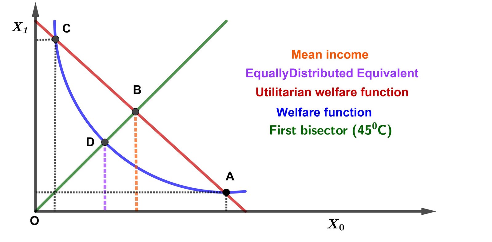
The basis of the measurement of Atkinson inequalities is based on the concept of equitably distributed equivalent income that we denote X*. Income X* is the income that, if all individuals had this amount, would give the same level of social utility as the existing one (W̄). Taking the case of two individuals, we can graphically represent the construction of the Atkinson index. Figure 1 illustrates this concept of equitably distributed equivalent. This graph shows the welfare function constructed on the space of individual incomes. The (Ox) axis shows the income of individual 1, while the (Oy) axis shows that of individual 2. If X0 is the income of the first individual and X1 that of the second, the average income is X̄. Suppose the income distribution is such that point A prevails i.e. the point where we have X0 > X1. In the absence of inequality aversion (θ = 0), utilitarian welfare would prevail i.e. the straight line. With this welfare function, the only way to have equal incomes at the same level of welfare is therefore to give an average income to both individuals i.e. X̄. Since inequality aversion is zero, we are not willing to reduce the size of the butter to have more equal shares. With inequality aversion, the convex welfare function would prevail. Now, starting from A, we can find a point where incomes are equally distributed at the same level of welfare. Since the welfare function is convex, income X* must be less than average income X̄. Income X* is the abscissa of point B of the 45 degree line that has the same social welfare as A and C. Even though total income (the sum of the two individual incomes) is less than XA, it is compensated by the gain in equality of the distribution. The reason being that, since inequality aversion is positive, we are now willing to pay the lower price of butter in order to have more equal shares. Equality is measured by the ratio X* / X̄. If this ratio is equal to 1 then each individual has the same level of income or if the welfare function is utilitarian (there is no perceived inequality). The approximative Atkinson inequality index can therefore be expressed as follows (see Bell et al. [11]):
\[ \tilde{A} = 1 – \frac{X^*}{\bar{X}}. \tag{6} \]Instinctively, this index tells us how much income we are willing to give up to have equal income. We therefore deduce that if the welfare is of the discrete form
\[ \tilde{W}(\theta) = \begin{cases} \frac{1}{n} \sum\limits_{i=1}^{n} \frac{X_i^{1 – \theta}}{1 – \theta} & \text{if } \theta \neq 1, \\ \frac{1}{n} \sum\limits_{i=1}^{n} \log(X_i) & \text{if } \theta = 1, \end{cases} \tag{7} \]then the discrete Atkinson index is given by:
\[ \tilde{A}(\theta) = \begin{cases} 1 – \left[ \frac{1}{n} \sum\limits_{i=1}^{n} \left( \frac{X_i}{\bar{X}} \right)^{1 – \theta} \right]^{\frac{1}{1 – \theta}}, & \text{if } \theta \neq 1, \\ 1 – \frac{1}{\bar{X}} \exp \left[ \frac{1}{n} \sum\limits_{i=1}^{n} \log(X_i) \right] & \text{if } \theta = 1. \end{cases} \tag{8} \]The formulas (or estimators if we can say so) [7] and [8] are the most used in the literature so far and would reveal inadequacies following the variation of the data since most of the data follow a distribution or at worst approximately a distribution. Hence the need to construct a non-parametric estimator or kernel estimator which often presents satisfactory results.
Kernel estimation (or Parzen–Rosenblatt method or KDE) is a non-parametric method for estimating the probability density of a random variable. It is based on a sample of a statistical population and makes it possible to estimate the density at any point of the support. In this sense, this method cleverly generalizes the histogram estimation method. Kernel density estimation is used to obtain a smooth estimate of the data distribution without making assumptions about the shape of the distribution and it is famous for its surprising smoothing character.
Let (Xi)1 ≤ i ≤ n be a random sample of size n from a population X with density function f, which represents the distribution of income. Xi, for i ∈ [[1,n]], designating the respective income of the n individuals, are independent and identically distributed (i.i.d.) observations. The main of nonparametric density estimation is to estimate f with as few assumptions about f as possible. Among the existing kernel density estimators, we choose the classic and most famous case well known in the literature, because of its simplicity for independent observations. This estimator depends on a parameter called smoothing parameter or bandwidth parameter. It is defined by:
\[ \hat{f}_n(x) = \frac{1}{n h} \sum_{i=1}^{n} K\left(\frac{x – X_i}{h}\right), \quad x \in \mathbb{R}, \tag{9} \]where h = h(n) = hn is the bandwidth parameter depending on the sample size n and K a probability density function called kernel function verifying certain particular properties called regularity properties.
From the estimator (9) of the distribution function f, it is obvious that we obtain an estimator of the Atkinson index [2], which is defined by:
\[ \tilde{A}_n(\theta) = 1 – \left[ \int_{\mathbb{R}} \left( \frac{x}{\tilde{\mu}_n} \right)^{1 – \theta} \hat{f}_n(x) dx \right]^{\frac{1}{1 – \theta}} = 1 – \left[ \frac{1}{n h} \sum_{i=1}^{n} \int_{\mathbb{R}} \left( \frac{x}{\tilde{\mu}_n} \right)^{1 – \theta} K\left( \frac{x – X_i}{h} \right) dx \right]^{\frac{1}{1 – \theta}}, \quad \text{if } \theta \neq 1, \tag{10} \]and
\[ \tilde{A}_n(1) = 1 – \frac{1}{\tilde{\mu}_n} \left[ \int_{\mathbb{R}} \log(x) \hat{f}_n(x) dx \right] = 1 – \frac{1}{\tilde{\mu}_n} \exp \left[ \frac{1}{n h} \sum_{i=1}^{n} \int_{\mathbb{R}} \log(x) K\left( \frac{x – X_i}{h} \right) dx \right], \tag{11} \]where 𝜇̃n is the estimator average income μ. It is easy to verify that 𝜇̃n satisfies:
\[ \tilde{\mu}_n = \int_{\mathbb{R}} x \hat{f}_n(x) dx = \frac{1}{n} \sum_{i=1}^{n} X_i, \tag{12} \]and consequently, we can obtain the nonparametric estimator of (5)
\[ \tilde{W}_n(\theta) = \begin{cases} [\tilde{\mu}_n (1 – \tilde{A}_n(\theta))]^{1 – \theta} & \text{if } \theta \neq 1, \\ \log[\tilde{\mu}_n (1 – \tilde{A}_n(\theta))] & \text{if } \theta = 1. \end{cases} \tag{13} \]The following paragraph provides a study of the near convergence or strong consistency of our estimators and also those of some estimators which will result from them under certain regularity hypotheses.
In all that follows, besides the classical regularity conditions (see in Agbokou [12]), well known in the literature, on the kernel function K and on the smoothing parameter h, we consider the following hypotheses.
A1. The random variable X takes values in ℝ+ or a compact subset of ℝ+.
A2. The density function f of X is uniformly continuous on its support and satisfies:
\[ \int_{\mathbb{R}} x^{\tau} f(x) = \mathbb{E}(X^{\tau}) > 0,\quad \forall\, \tau > 0. \]A4. There exists a strictly positive constant η such that μ > η and θ takes values in [0;1].
A5. The function φ : y ↦ yt on ℝ+ verifies the following conditions:
K is a symmetric Kernel of bounded variation on ℝ vanishing outside the interval [a, +a] for some a > 0 and satisfying:
The bandwidth parameter h = (hn)n∈ℕ is a sequence of positive nonincreasing real numbers satisfying:
Remark 1. The assumptions A1 – A2, K1 – K2 and H2 are quite standard. A1 – A4, A5.i and iii, K1 – K3 and H1 – H2 ensure the strong uniform convergence of the estimators [10] and [11] to [2] and [4] respectively. Finally all the assumptions ensure the strong uniform convergence of [13] to [5].
Note 1. To simplify the writings and make them easier to handle, we adopt the following notations:
Consequently, it is clear that their kernel estimators are respectively \(\tilde{A}_n(\theta)\) and \(\tilde{\Lambda}_n\).
In this subsection, we prove the consistency of our estimator and give a rate of convergence. Our first result is the almost sure uniform convergence with an appropriate rate of the estimators \(\tilde{A}_n\) and \(\tilde{\Lambda}_n\) stated in Proposition 1, which are the key for investigating the strong consistency of \(\tilde{A}_n(\theta)\) and \(\tilde{A}_n(1)\) given by Theorem 1. The last result deals with the strong consistency of the welfare function estimator \(\tilde{W}_n(\theta)\) given by Corollary.
Proposition 1. Under assumptions A1, A5 – iii, K1, K3 and H1 we have:
(i)
\[ |\tilde{A}_n(\theta) – \Delta(\theta)| \longrightarrow 0 \text{ a.s.}, \quad n \rightarrow +\infty \quad \forall\, \theta \in [0,1[. \tag{14} \](ii) In particular for \(\theta = 1\), we have:
\[ |\tilde{\Lambda}_n – \Lambda| \longrightarrow 0 \text{ a.s.}, \quad n \rightarrow +\infty. \tag{15} \]The Proposition 1 leads to the convergence of the inequality index function which is established by the following theorem:
Theorem 1. In addition to the assumptions of the Proposition 1, if hypotheses A2, A4 – A5–i, K2 and H2 are satisfied, then we obtain:
(i)
\[ |\tilde{A}_n(\theta) – A(\theta)| \longrightarrow 0 \text{ a.s.}, \quad n \rightarrow +\infty \quad \forall\, \theta \in [0,1[. \tag{16} \](ii) In particular, if \(\theta = 1\), then we get:
\[ |\tilde{A}_n(1) – A(1)| \longrightarrow 0 \text{ a.s.}, \quad n \rightarrow +\infty. \tag{17} \]As a consequence of the Theorem 1, we arrive at the strong constancy of the estimator of the welfare function (13).
Corollary 1. Under the same hypotheses as Theorem 1, assume that hypothesis A5–ii is verified, then we obtain:
\[ |\tilde{W}_n(\theta) – W(\theta)| \longrightarrow 0 \text{ a.s.}, \quad n \rightarrow +\infty \quad \forall\, \theta \in [0,1]. \tag{18} \]Corollary 2. Under the same assumptions as Theorem 1, we assume that the sequence \((X_i)_{1 \leq i \leq n}\) of i.i.d. random variables is such that \(\mathbb{E}(X_i) = \mu\) and \(\text{Var}(X_i) = \sigma^2\quad \forall\, i \in \{1,\dots,n\}\). Then for \(n\) large enough, we get:
\[ \tilde{A}_n(\theta) – A(\theta) \longrightarrow \mathcal{N}(0, s^2) \quad \text{a.s.} \quad \forall\, \theta \in [0,1], \tag{19} \]where
\[ s^2 = (1 + \mu^2) \left( 1 + \frac{\sigma^2}{\mu^2} \right). \]As for the proofs of the previous proposition, theorem and corollary, we need some very important or primordial lemmas whose demonstrations will be made or will be given here as well.
Let us first recall that if \(\{X_i\}_{1}^{n}\) are i.i.d random variables with a distribution F. Consider a parametric function \(\Pi\) for which there exists an unbiased estimator. The parametric function \(\Pi\) can be expressed in the following form:
\[ \Pi(F) = \mathbb{E}[\psi(X_1,\dots,X_l)] = \int_{\mathbb{R}^l} \psi(X_1,\dots,X_l) dF(x_1) \cdots dF(x_l), \]where \(\psi\) is a function of \(l\) i.i.d random variables from \(\{X_i\}_{1}^{n}\) with \(l \leq n\). For any function \(\Psi\), the corresponding U-statistic for the estimation of \(\Pi\) based on a random sample of size \(n\) is obtained by averaging \(\Psi\) symmetrically over the observations:
\[ U_n = U(X_1, \dots, X_n) = \frac{1}{\binom{n}{l}} \sum_{s} \psi(X_1, \dots, X_l), \]where \(\sum_{s}\) represents the summation over the \(\binom{n}{l}\) combinations of \(l\) distinct elements \(i_j,\quad j \in \{1, \dots, l\}\) from \(\{1,\dots,n\}\). In particular, we have:
Lemma 1. For \(\psi(x) = x^m\) \((m > 0)\), the corresponding U-statistic is
\[ U_m = U(X_1, \dots, X_n) = \frac{1}{n} \sum_{i=1}^{n} X_i^m, \]and for \(n\) large enough, we get
\[ U_m \longrightarrow \mu_m = \mathbb{E}[X^m] = \int_{\mathbb{R}} x^m dF(x). \]In particular for \(m = 1\), we set \(\tilde{\mu}_n = U_1 \longrightarrow \mu = \mu_1\).
Proof. The proof of this lemma is similar to those found in Serfling [13] and Lehmann [14]. Thus we make an exception to this one.
Lemma 2. For every \(p \in ]0;1]\), the function defined on \(I = [0; +\infty)\) by \(\Phi : z \mapsto z^p\) satisfies the following condition:
\[ \forall\, u, v \in I : |\Phi(u) – \Phi(v)| \leq p |u – v|^{p}, \tag{20} \]and the number \(p\) is the maximum of all values that verify this property.
Proof. For \(u, v\) let us suppose that \(u > v\). Aware that \(p – 1 \leq 0\), we have
\[ |\Phi(u) – \Phi(v)| = u^p – v^p = \int_{v}^{u} p z^{p-1} dz \] \[ \leq \int_{v}^{u} p(z – v)^{p-1} dz = (u – v)^p \] \[ \leq |u – v|^p \quad \text{because } u > v. \]In this case, the corresponding \(p\) of the inequality (20) which satisfies the condition is equal to 1. On the other hand, from the relation (20), setting \(u = 1\) and \(v = 0\), it follows \(p > 1\).
Now assume that \(p > 1\). If there exists another real number \(q\) such that \(q > p\) and verifies the inequality (20), then we obtain
\[ \forall\, u, v \in I : |\Phi(u) – \Phi(v)| \leq q |u – v|^{q}. \tag{21} \]By setting \(v = 0\) in relation (21), we have
\[ |\Phi(u)| = u^p \leq u^q \quad \forall\, u > 0. \]Taking into account that \(p – q < 0\), we get \(u^{p-q} < q\). This is absurd because the left-hand side diverges towards \(+\infty\) when \(u\) tends towards 0. This brings the proof of this lemma to term.
The lemmas having been established, let’s move on to the proofs of the main results obtained.
Proof of Proposition 1. (i) From the sequence of functions \(\tilde{\Delta}_n\) in \(\theta\), we obtain
\[ \tilde{\Delta}_n(\theta) = \int_{\mathbb{R}} x^{1-\theta} \hat{f}_n(x)\,dx = \frac{1}{nh} \sum_{i=1}^{n} \int_{\mathbb{R}} x^{1-\theta} K\left( \frac{x – X_i}{h} \right) dx. \]A change of variable, the use of hypotheses and A5–ii, K1 – K3, allows us to write successively
\[ \tilde{\Delta}_n(\theta) = \frac{1}{n} \sum_{i=1}^{n} \int_{\mathbb{R}} (X_i + wh)^{1 – \theta} K(w)\,dw \] \[ \leq Q_{1 – \theta} \cdot \frac{1}{n} \sum_{i=1}^{n} \int_{\mathbb{R}} \left( X_i^{1 – \theta} + w^{1 – \theta} h^{1 – \theta} \right) K(w)\,dw \] \[ \leq Q_{1 – \theta} \left[ \frac{1}{n} \sum_{i=1}^{n} X_i^{1 – \theta} + h^{1 – \theta} \int_{\mathbb{R}} w^{1 – \theta} K(w)\,dw \right] \] \[ \leq Q_{1 – \theta} \left[ U_{1 – \theta} + h^{1 – \theta} \nu_{\theta}(K) \right]. \]Then we get
\[ |\tilde{\Delta}_n(\theta) – U_{1 – \theta}| \leq M h^{1 – \theta} \quad \text{where } M > 0 \text{ is a constant}. \]In other words
\[ |\tilde{\Delta}_n(\theta) – U_{1 – \theta}| = \mathcal{O}(h^{1 – \theta}) \quad \text{a.s.} \]Furthermore, we have
\[ |\tilde{\Delta}_n(\theta) – \Delta(\theta)| \leq |\tilde{\Delta}_n(\theta) – U_{1 – \theta}| + |U_{1 – \theta} – \Delta(\theta)|. \tag{22} \]For \(n\) large enough and under hypothesis \(H_1\), Lemma 1 applied to inequality (22) completes the first part (i) of the proof of this proposition.
(ii) The second part is inspired by the first, with a few exceptions since it is a special case. Since function \(z \mapsto \exp(z)\) is a convex function, Jensen’s inequality allows us to write
\[ \tilde{\Lambda}_n = \exp \left[ \int_{\mathbb{R}} \log(x) \hat{f}_n(x)\,dx \right] \leq \frac{1}{nh} \sum_{i=1}^{n} \int_{\mathbb{R}} x K\left( \frac{x – X_i}{h} \right) dx. \]The same change of variable and the use of the same hypotheses lead to
\[ \tilde{\Lambda}_n \leq \frac{1}{n} \sum_{i=1}^{n} X_i + h \int_{\mathbb{R}} w K(w)\,dw \leq U_1 + h \nu(K) \quad \text{because here } w > 0, \]now we get
\[ |\tilde{\Lambda}_n – U_1| \leq Mh \quad \text{where } M > 0 \text{ is a constant}. \]By using a similar inequality like that of (22) with \(\tilde{\Lambda}_n, \Lambda\) and \(U_1\), Lemma 1 and hypothesis \(H_1\) complete the last part of this proposition for \(n\) large enough.
(i) Thanks to hypothesis A2, A5–i, we can write
\[ |\tilde{A}_n(\theta) – A(\theta)| = \left| \left[ \frac{\tilde{\Delta}_n}{\tilde{\mu}_n^{1 – \theta}} \right]^{\frac{1}{1 – \theta}} – \left[ \frac{\Delta}{\mu^{1 – \theta}} \right]^{\frac{1}{1 – \theta}} \right| \] \[ \leq \left( \frac{1}{1 – \theta} \right) K \left| \frac{\tilde{\Delta}_n}{\tilde{\mu}_n^{1 – \theta}} – \frac{\Delta}{\mu^{1 – \theta}} \right| \] \[ \leq \left( \frac{1}{1 – \theta} \right) K \left\{ \frac{\mu^{1 – \theta}}{\tilde{\mu}_n^{1 – \theta}} \cdot \frac{1}{\mu^{1 – \theta}} + \frac{1}{\lim\inf_{n \to +\infty} \tilde{\mu}_n^{1 – \theta}} |\tilde{\Delta}_n – \Delta| \right\} \] \[ \leq M \left| \frac{1}{\tilde{\mu}_n^{1 – \theta}} – \frac{1}{\mu^{1 – \theta}} \right| + |\tilde{\Delta}_n – \Delta|. \]where \[ 0 < M = \max \left\{ \mu^{1 – \theta}; \frac{1}{\lim\inf_{n \to +\infty} \tilde{\mu}_n^{1 – \theta}} \right\} \times \left( \frac{1}{1 – \theta} \right)^K. \]
Lemma 1 associated with the Mapping Theorem allows us to obtain
\[ \left| \frac{1}{\tilde{\mu}_n^{1 – \theta}} – \frac{1}{\mu^{1 – \theta}} \right| \rightarrow 0, \quad \text{a.s.} \quad n \rightarrow +\infty. \tag{23} \]Thus (23) and Proposition 1 – (i) completes the first part of this theorem.
(ii) As previously in (i), the same assumptions give us:
\[ |\tilde{A}_n(1) – A(1)| = \left| \frac{\tilde{\Lambda}_n}{\tilde{\mu}} – \frac{\Lambda}{\mu} \right| \] \[ \leq \mu \left| \frac{1}{\tilde{\mu}} – \frac{1}{\mu} \right| + \frac{1}{\lim\inf_{n \to +\infty} \tilde{\mu}_n} |\tilde{\Lambda}_n – \Lambda| \] \[ \leq M \left( \left| \frac{1}{\tilde{\mu}} – \frac{1}{\mu} \right| + |\tilde{\Lambda}_n – \Lambda| \right) \]where \[ 0 < M = \left\{ \mu; \frac{1}{\lim\inf_{n \to +\infty} \tilde{\mu}_n} \right\}. \]
As previously in proof (i), Lemma 1 associated with the mapping theorem and Proposition 1-(ii) complete the last part of this theorem.
(i) This first part will concern the case where \(\theta \in [0;1[\). Lemma 2 and the Triangle Inequality lead us to
\[ |\tilde{W}_n(\theta) – W(\theta)| = \left| [\tilde{\mu}_n (1 – \tilde{A}_n(\theta)) ]^{1 – \theta} – [\mu(1 – A(\theta)) ]^{1 – \theta} \right| \] \[ \leq (1 – \theta) |\bar{z}| (1 – \tilde{A}_n(\theta) – (1 – A(\theta)))^{1 – \theta} \] \[ \leq (1 – \theta) \left\{ (1 + A(\theta)) |\tilde{\mu}_n – \mu| + \tilde{\mu}_n |\tilde{A}_n(\theta) – A(\theta)| \right\} \] \[ \leq M_{\theta} \left\{ |\tilde{\mu}_n – \mu| + |\tilde{A}_n(\theta) – A(\theta)| \right\}, \]where \[ 0 < M_{\theta} = \max \left\{ 1 + A(\theta); \lim\sup_{n \to +\infty} \tilde{\mu}_n \right\} \times (1 – \theta), \quad \forall\, \theta \in [0;1[. \]
Thus Lemma [1] and Theorem 1 – (i) complete the first part of this corollary.
(ii) This second and last part concerns the case where \(\theta = 1\). For this case especially, we assume that \(A(1)\) and its estimator \(\tilde{A}_n(1)\) are all different from 1 or all do not approach 1. Therefore \(\mu(1 – A(1))\) and \(\tilde{\mu}_n(1 – \tilde{A}_n(1))\) are strictly positive. Let us denote \(\delta = \min \left\{ \mu(1 – A(1)); \tilde{\mu}_n(1 – \tilde{A}_n(1)) \right\}\). We therefore have \(\delta\) strictly positive.
Thus the function \(z \mapsto \log(z)\) is \(\frac{1}{\delta}\)-Lipschitzian on \([\delta; +\infty[\) because its derivative in absolute value is bounded above by \(\frac{1}{\delta}\). This leads us to write:
\[ |\tilde{W}_n(1) – W(1)| = \left| \log [\tilde{\mu}_n (1 – \tilde{A}_n(1))] – \log[\mu (1 – A(1))] \right| \] \[ \leq \frac{1}{\delta} |\tilde{\mu}_n (1 – \tilde{A}_n(1)) – \mu (1 – A(1))| \] \[ \leq M_{\delta} \left\{ |\tilde{\mu}_n – \mu| + |\tilde{A}_n(1) – A(1)| \right\}, \]where
\[ 0 < M_{\delta} = \max \left\{ 1 + A(1); \lim\sup_{n \to +\infty} \tilde{\mu}_n \right\} \div \delta. \]Thus Lemma [1] and Theorem 1 – (ii) complete the last part of this corollary.
◦ For \(\theta \in [0,1[\), we directly and successively draw these inequalities from the following relation (see proof of the Proposition 1):
\[ \tilde{\Delta}_n(\theta) \leq Q_{1 – \theta} \left[ \frac{1}{n} \sum_{i=1}^{n} X_i^{1 – \theta} + h^{1 – \theta} \int_{\mathbb{R}} w^{1 – \theta} K(w)\,dw \right]. \]Using the property of monotonic increasing and the linearity of the mathematical expectation and also \(\|a – b\| \leq |a – b|\), then we have
\[ \mathbb{E}[\tilde{\Delta}_n(\theta)] \leq Q_{1 – \theta} \mathbb{E}[X^{1 – \theta}] + h^{1 – \theta} Q_{1 – \theta} \nu(K) \Rightarrow \mathbb{E}[|\tilde{\Delta}_n(\theta) – \Delta(\theta)|] = \mathcal{O}(h^{1 – \theta}). \tag{24} \]Moreover, we have
\[ |\tilde{A}_n(\theta) – A(\theta)| \leq M \left[ \left| \frac{1}{\tilde{\mu}_n} – \frac{1}{\mu} \right| + |\tilde{\Delta}_n(\theta) – \Delta(\theta)| \right] \] \[ \Rightarrow \mathbb{E}[|\tilde{A}_n(\theta) – A(\theta)|] \leq M \left[ \mathbb{E} \left| \frac{1}{\tilde{\mu}_n} – \frac{1}{\mu} \right| + \mathbb{E}[|\tilde{\Delta}_n(\theta) – \Delta(\theta)|] \right] \]Thus for \(n\) large enough, we have \(\mathbb{E}[|\tilde{A}_n(\theta) – A(\theta)|] \longrightarrow 0\). In particular we obtain
\[ \mathbb{E}[ \tilde{A}_n(\theta) – A(\theta) ] \longrightarrow 0 \iff \mathbb{E}[ \tilde{A}_n(\theta) ] = A(\theta). \tag{25} \]We have just shown that the estimator is asymptotically unbiased. We can notice that \((a – b)^2 \leq a^2 + b^2\) (where \(a\) and \(b\) have the same sign) and also the function \(z \mapsto z^p\), \(p \geq 2\) is convex (this allows us to apply Jensen’s inequality). All this allows us to write
\[ \left( \tilde{A}_n(\theta) – A(\theta) \right)^2 \leq \left[ \left( \int_{\mathbb{R}} \left( \frac{x}{\tilde{\mu}_n} \right)^{1 – \theta} \hat{f}_n(x)\,dx \right)^{\frac{1}{1 – \theta}} + \left( \int_{\mathbb{R}} \left( \frac{x}{\mu} \right)^{1 – \theta} f(x)\,dx \right)^{\frac{1}{1 – \theta}} \right]^2 \] \[ \leq \left( \int_{\mathbb{R}} \left( \frac{x}{\tilde{\mu}_n} \right)^2 \hat{f}_n(x)\,dx + \int_{\mathbb{R}} \left( \frac{x}{\mu} \right)^2 f(x)\,dx \right) \] \[ \leq \frac{1}{n} \sum_{i=1}^{n} X_i^2 \int_{\mathbb{R}} K(w)\,dw + 2 h^{1 – \theta} \frac{1}{n} \sum_{i=1}^{n} X_i^2 \int_{\mathbb{R}} w K(w)\,dw + h^2 \int_{\mathbb{R}} w^2 K(w)\,dw + \frac{\mu_2}{\mu^2} \] \[ \Rightarrow \mathbb{E} \left[ \left( \tilde{A}_n(\theta) – A(\theta) \right)^2 \right] = \mu^2 + \frac{\mu_2}{\mu^2} + \mathcal{O}(h^2) = (\mu^2 + 1) \left( 1 + \frac{\sigma^2}{\mu^2} \right) + \mathcal{O}(h^2). \]Furthermore we know that
\[ \text{Var}[\tilde{A}_n(\theta) – A(\theta)] = \mathbb{E} \left[ (\tilde{A}_n(\theta) – A(\theta))^2 \right] – \mathbb{E}^2[\tilde{A}_n(\theta) – A(\theta)]. \]So, from the relation (24) we have
\[ \text{Var}[\tilde{A}_n(\theta) – A(\theta)] = (\mu^2 + 1)\left(1 + \frac{\sigma^2}{\mu^2}\right) + \mathcal{O}(h^{2 – 2\theta}) \quad \text{a.s.} \tag{26} \]For \(n\) large enough, we have \(\text{Var}[\tilde{A}_n(\theta) – A(\theta)] \longrightarrow s^2 = (\mu^2 + 1)\left(1 + \frac{\sigma^2}{\mu^2}\right)\).
◦ For \(\theta = 1\), we also have (see proof of Proposition 1):
\[ \tilde{\Lambda}_n \leq \frac{1}{n} \sum_{i=1}^{n} X_i + h \int_{\mathbb{R}} w K(w)\,dw \Rightarrow \mathbb{E}[\tilde{\Lambda}_n] \leq \mathbb{E}[X_i] + h\nu(K) \Rightarrow \mathbb{E}[\tilde{\Lambda}_n – \mu] = \mathcal{O}(h) \quad \text{a.s.} \]On the one hand, the convexity of the exponential function, the triangular inequality and \(\|a – b\| \leq |a – b|\) allows us to have
\[ \mathbb{E}|\tilde{\Lambda}_n – \Lambda| \leq \mathbb{E}|\tilde{\Lambda}_n – \mu| + \mathbb{E}|\Lambda – \mu| \Rightarrow \mathbb{E}|\tilde{\Lambda}_n – \Lambda| = \mathcal{O}(h) \quad \text{a.s.} \]On the other hand
\[ |\tilde{A}_n(1) – A(1)| \leq M \left( \left| \frac{1}{\tilde{\mu}} – \frac{1}{\mu} \right| + |\tilde{\Lambda}_n – \Lambda| \right) \]Thus, for \(n\) large enough
\[ \mathbb{E}[ \tilde{A}_n(1) – A(1) ] = \mathcal{O}(h) \quad \text{a.s.} \tag{27} \]We have also
\[ (\tilde{A}_n(\theta) – A(\theta))^2 \leq \left( \frac{1}{\tilde{\mu}_n} \exp \left[ \int_{\mathbb{R}} \log(x) \hat{f}_n(x)\,dx \right] \right)^2 + \left( \frac{1}{\mu} \exp \left[ \int_{\mathbb{R}} \log(x) f(x)\,dx \right] \right)^2 \] \[ \leq \frac{1}{\tilde{\mu}_n^2} \exp \left[ 2 \int_{\mathbb{R}} \log(x) \hat{f}_n(x)\,dx \right] + \frac{1}{\mu^2} \exp \left[ 2 \int_{\mathbb{R}} \log(x) f(x)\,dx \right] \] \[ \leq \frac{1}{\tilde{\mu}_n^2} \int_{\mathbb{R}} x^2 \hat{f}_n(x)\,dx + \frac{\mu_2}{\mu^2} \Rightarrow \mathbb{E}\left[(\tilde{A}_n(\theta) – A(\theta))^2\right] \leq M \left[ \mu_2 + h^2 \nu(K) \right] + \frac{\mu_2}{\mu^2}. \]For n large enough, we get
\[ \Rightarrow \mathbb{E} \left[ (\tilde{A}_n(\theta) – A(\theta))^2 \right] = \mu_2 + \frac{\mu_2}{\mu^2} + \mathcal{O}(h^2) \quad \text{a.s.} \tag{28} \]
Formulas (27) and (28) give the variance as previously \[ \text{Var}[\tilde{A}_n(\theta) – A(\theta)] = (1 + \mu^2) \left( 1 + \frac{\sigma^2}{\mu^2} \right) + \mathcal{O}(h^2) \quad \text{a.s.} \]
This which completes the proof of this corollary.
Before moving on to numericals, we were able to calculate the Atkinson inequality index and welfare for certain probability distributions that will be useful for the rest.
However, theoretical calculations of the Atkinson index with probability distributions are not easy or easy to determine. With other distributions, this seems very complex or even impossible. We will spare you these details and the results obtained are grouped in the Table 1.
The theoretical calculation of the Atkinson index involves certain so-called special functions which are defined by:
| Name | p.d.f. \( f(x) \) | Atkinson index \( A(\theta) \) | Welfare function \( W(\theta) \) |
|---|---|---|---|
| Beta \( \mathcal{B}(\alpha, \beta) \) | \[ \frac{1}{\mathcal{B}(\alpha, \beta)} x^{\alpha – 1} (1 – x)^{\beta – 1} \mathbf{1}_{[0,1]}(x) \] | \[
1 – \frac{\alpha + \beta}{\alpha}
\cdot \frac{\Gamma(\alpha + 1 – \theta)\Gamma(\beta)}{\mathcal{B}(\alpha, \beta)\Gamma(\alpha + \beta + 1 – \theta)}
\quad \theta \ne 1
\] \[ 1 – \frac{\alpha + \beta}{\alpha} \exp[\psi(\alpha) – \psi(\alpha + \beta)] \quad \theta = 1 \] |
\[
\frac{\Gamma(\alpha + 1 – \theta)\Gamma(\beta)}{\mathcal{B}(\alpha, \beta)\Gamma(\alpha + \beta + 1 – \theta)}
\quad \theta \ne 1
\] \[ \psi(\alpha) – \psi(\alpha + \beta) \quad \theta = 1 \] |
| Exponential \( \mathcal{E}(\lambda) \) | \[ \lambda e^{-\lambda x} \mathbf{1}_{[0,+\infty[}(x) \] | \[
1 – \lambda^{\theta} \Gamma(1 – \theta)
\quad \theta \ne 1
\] \[ 1 – \lambda \exp(-\gamma) \quad \theta = 1 \] |
\[
\frac{\Gamma(2 – \theta)}{\lambda^{1 – \theta}}
\quad \theta \ne 1
\] \[ \frac{1}{\lambda}(\gamma) \quad \theta = 1 \] |
| Gamma \( \Gamma(\alpha, \beta) \) | \[ \frac{\beta^\alpha}{\Gamma(\alpha)} x^{\alpha – 1} e^{-\beta x} \mathbf{1}_{[0,+\infty[}(x) \] | \[
1 – \frac{\Gamma(\alpha + 1 – \theta)}{\beta^{1 – \theta}\Gamma(\alpha)}
\quad \theta \ne 1
\] \[ 1 – \exp[\psi(\alpha) – \log(\beta)] \quad \theta = 1 \] |
\[
\frac{\Gamma(\alpha + 1 – \theta)}{\beta^{1 – \theta}}
\quad \theta \ne 1
\] \[ \psi(\alpha) – \log(\beta) \quad \theta = 1 \] |
| Pareto \( \mathcal{P}(\alpha, \beta) \) | \[ \frac{\alpha \beta^\alpha}{x^{\alpha + 1}} \mathbf{1}_{[\beta,+\infty[}(x) \] | \[
1 – \left( \frac{\alpha – 1}{\alpha – \theta} \right)^{1 – \theta}
\quad \theta \ne 1
\] \[ 1 – \exp\left[\frac{1}{\alpha – 1} + \log(\alpha – 1)\right] \quad \theta = 1 \] |
\[
\frac{(\alpha – 1)^{1 – \theta}}{\alpha – \theta}
\quad \theta \ne 1
\] \[ \frac{1}{\alpha – 1} + \log(\alpha – 1) \quad \theta = 1 \] |
| Uniform \( \mathcal{U}([a, b]) \) | \[ \frac{1}{b – a} \mathbf{1}_{[a,b]}(x) \] | \[
1 – \left( \frac{b^{2 – \theta} – a^{2 – \theta}}{(2 – \theta)(b – a) \bar{x}^{1 – \theta}} \right)^{\frac{1}{1 – \theta}}
\quad \theta \ne 1
\] \[ 1 – \exp\left[ \frac{b \log(b) – a \log(a)}{b – a} – 1 \right] \quad \theta = 1 \] |
\[
\frac{b^{2 – \theta} – a^{2 – \theta}}{(2 – \theta)(b – a)}
\quad \theta \ne 1
\] \[ \frac{b \log(b) – a \log(a)}{b – a} – 1 \quad \theta = 1 \] |
| Weibull \( \mathcal{W}(\alpha, \beta) \) | \[ \frac{\alpha}{\beta} \left( \frac{x}{\beta} \right)^{\alpha – 1} \exp\left[-\left(\frac{x}{\beta}\right)^\alpha\right] \mathbf{1}_{[0,+\infty[}(x) \] | \[
1 – \left( \frac{\Gamma(1 + 1/\alpha)}{\beta} \right)^{1 – \theta} \left( \frac{1}{\beta^{1 – \theta}} \right)
\quad \theta \ne 1
\] \[ 1 – \exp\left[\frac{\gamma}{\alpha} + \log(\beta)\right] \quad \theta = 1 \] |
\[
\beta^{1 – \theta} \Gamma\left(1 + \frac{1 – \theta}{\alpha}\right)
\quad \theta \ne 1
\] \[ \frac{1}{\alpha} + \log(\beta) + \gamma \quad \theta = 1 \] |
Remark 2. Recall that the first lines of the expressions that are in the braces represent the general case for θ ≠ 1. and those of the second lines represent the particular case for θ = 1.
The table being obtained, we choose one of these models to study the cobergence of our nonparametric estimator with respect to that. Our choice is the Weibull model because of its particularity in terms of application and its multitasking. The Weibull distribution intervenes in almost all areas like that of Pareto in the estimations of income inequality measures (see Agbokou [4]). To do this, with the data we have, we will determine these parameters by the Maximum Likelihood (M.L.) method to obtain the theoretical Atkinson index.
Due to its adaptability in fitting distributions or data particularly in data science, the Weibull distribution has taken in recent years a major position in the field of parametric, semi or nonparametric estimations. One of the main barriers to a more important or wider use of the Weibull distribution is the complexity of estimating its parameters. Regrettably or sadly, the calculations that this estimation involves are not always simple enough. This subsection deals with the estimation of maximum likelihood in samples of the Weibull probability density. The likelihood function of this sample \((X_{1},\cdots,X_{n})\) is given by:
\[L(X_{1},\cdots,X_{n},(\alpha,\beta))=\Pi_{i=1}^{n}\frac{\alpha}{\beta}X_{i}^{\alpha-1}\exp\left(-\frac{X_{i}^{\alpha}}{\beta}\right).\]
We let \(\mathcal{L}(\alpha,\beta)=\mathcal{L}(X_{1},\cdots,X_{n},(\alpha,\beta))=\log L( X_{1},\cdots,X_{n},(\alpha,\beta))\) represent the log-likelihood, then we derive \(\mathcal{L}(\alpha,\beta)\) respectively with respect to \(\alpha\) and with respect to \(\beta\) then by setting the two partial derivatives equal to zero each, we obtain:
\[\left\{\begin{array}[]{l}\dfrac{\partial\mathcal{L}(\alpha,\beta)}{\partial \alpha}=\dfrac{n}{\alpha}+\sum\limits_{i=1}^{n}\log(X_{i})-\dfrac{1}{\beta} \sum\limits_{i=1}^{n}X_{i}^{\alpha}\log(X_{i})=0,\\ \dfrac{\partial\mathcal{L}(\alpha,\beta)}{\partial\beta}=-\dfrac{n}{\beta}+ \dfrac{1}{\beta^{2}}\sum\limits_{i=1}^{n}X_{i}^{\alpha}=0.\end{array}\right.\tag{29}\]
On eliminating \(\beta\) between these two equations of the system (29) and simplifying the term, we get:
\[ \frac{\sum\limits_{i=1}^{n} X_i^{\hat{\alpha}} \log(X_i)}{\sum\limits_{i=1}^{n} X_i^{\hat{\alpha}}} – \frac{1}{\hat{\alpha}} – \frac{1}{n} \sum\limits_{i=1}^{n} \log(X_i) = 0. \tag{30} \]We note that equation (30) is difficult or even impossible to solve analytically. We will therefore use a numerical resolution or iterative methods such as the Newton method or the fixed point method or the secant and regula falsi method in order to find the estimator \(\hat{\alpha}\) of the parameter \(\alpha\). If the estimator \(\hat{\alpha}\) is obtained, we therefore deduce from (29), the estimator \(\hat{\beta}\) of \(\beta\) by the equality:
\[ \hat{\beta} = \left( \frac{1}{n} \sum\limits_{i=1}^{n} X_i^{\hat{\alpha}} \right)^{\frac{1}{\hat{\alpha}}}. \tag{31} \]For our study, we focused on the World Bank data that could be easily found on their website DataBank [1]. We were interested in the “adjusted net national income per capita (current US dollars)” of 2021 for each country in the world (at least for those who have it because we could not find the updated data for all countries). Since the data is allocated by region according to the World Bank’s breakdown, we organized this data by continent as follows:
Remark 3. The last two groupings aim not only to study the inequalities of countries between two countries or between countries of the world but also to see the performance of our estimators when the sample size increases and also the impact of the inversion parameter on them depending on these sizes.
Table 2 provides a statistical description of some position and dispersion characteristics of these data taken to the thousandth in order to facilitate the calculations of the programming in the rest of this subsection using Matlab software.
In view of the statistical summary of Table 2, we notice that the data, whatever the area, are very heterogeneous since the coefficient of variation of each of these groupings is strictly greater than 0.30. This heterogeneity character makes this study very exciting since with simulated data (which we do not present here), we always had homogeneous data which contribute to the robustness of our estimators from the size n = 30. Thus the other objective is to see the behavior of our estimators facing heterogeneous data because we know that heterogeneous data in statistical study such as estimates and forecasts negatively affect or slow down the robustness of the estimators and by ricochet impact the forecasts.
| Statistic summary | Size | Minimum | Mean | Median | Mode | Maximum | Coefficient of variation |
|---|---|---|---|---|---|---|---|
| European area | 27 | 7.6500 | 25.3004 | 19.6460 | 7.6500 | 65.3640 | 0.5857 |
| America area | 33 | 1.2510 | 10.6735 | 6.0800 | 2.5109 | 52.6190 | 0.9870 |
| Asia area | 51 | 0.3400 | 9.7364 | 3.5040 | 0.3400 | 44.5130 | 0.7573 |
| Africa area | 54 | 0.1560 | 1.9479 | 1.1545 | 0.1560 | 7.1950 | 0.7712 |
| Eurasian area | 78 | 0.3400 | 15.1239 | 9.0055 | 0.3400 | 65.3640 | 0.8936 |
| World | 165 | 0.1560 | 9.9217 | 4.1900 | 0.4860 | 65.3640 | 0.7618 |
Thus, for the simulation of our estimators, we chose as a statistical kernel K, the Epanechnikov kernel also called the “parabolic” kernel. It is named after the author Epanechnikov [15], who used and studied it for the first time in 1969. On the one hand, it is well known in the literature that the kernel has little influence on the performance of nonparametric estimators. What motivates this choice is that this kernel allows to have the most efficient estimator for the density, which concerns us in this document. On the other hand, the literature reveals that the choice of the smoothing parameter h = hn has a major influence on the robustness of the kernel estimator (see Agbokou et al. [16, 17]). The process of this choice in the presence of real data is not as easy as in the presence of simulated data. We therefore opted for the numerical cross-validation method which consists in minimizing the integrated squared error defined from a series of observations or data (xi)1≤i≤qn of size n.
This error is defined by:
\[ \Phi(h_n) = \int_{x_{(1)}}^{x_{(n)}} \left( \widehat{A}_n(\theta) – A(\theta) \right)^2 dx, \tag{32} \]where x(1) = min(xi) and x(n) = max(xi) for all i ∈ {1, .., n}.
The bandwidth parameter selection rule results in the minimization of this criterion:
\[ \widehat{h}_n = \arg \min_{h_n} \Phi(h_n). \tag{33} \]The smoothing parameter of (33) thus obtained is asymptotically optimal. To determine the parameter h, our Matlab code is programmed in such a way that we obtain at the same time the RMSE (Residual Mean Square Error). This is the root mean square deviation, which is the standard deviation of the residuals (prediction errors). The residuals are the measure of the deviation between the data points and the regression line. The RMSE metric is the measure of this difference across these residuals. In other words, it indicates the concentration of the data around the line of best fit. In our work we have two parameters h to determine and therefore two RMSEs. We denote them respectively h1n for the estimator of the Atkinson index and h2n for its associated welfare function. Similarly, their errors or residuals are respectively noted RMSE1 and RMSE2.
To get an idea of the impact of the aversion parameter, we chose the parameter θ such that θ ∈ {0.01, 0.05, 0.1, 0.5, 0.9, 1} for each sample size (or area or region). We also calculated for each θ the classical estimators (usual classical forms) of the Atkinson index [8] and its welfare function [7] in order to see if they best estimate the theoretical Atkinson index and its theoretical welfare function.
Let us recall that the two parameters of the theoretical Atkinson index and its theoretical welfare function cannot be taken arbitrarily, we opted for the maximum likelihood (M.L.) method with the intervention of Newton’s numerical method in order to be able to assign a value to each of these parameters.
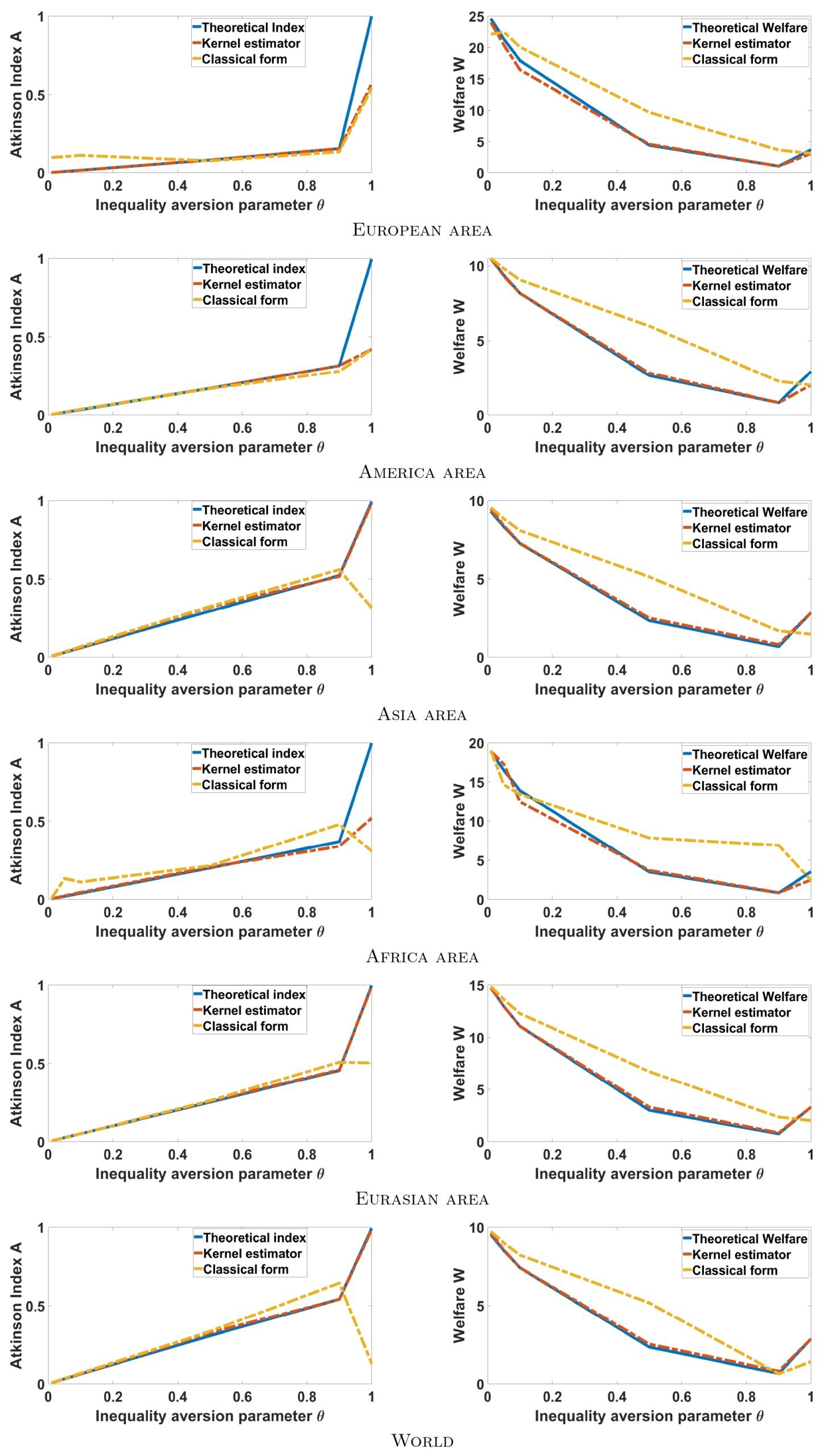
The results obtained are summarized in Table 3. A visualization of all these results obtained is summarized in Figure 2.
| θ | ĥ1n | ĥ2n | α̂ | β̂ | A(θ) | Ân(θ) | Ã(θ) | W(θ) | Ŵn(θ) | W̃(θ) | RMSE1 | RMSE2 |
|---|---|---|---|---|---|---|---|---|---|---|---|---|
| European area | ||||||||||||
| 0.01 | 0.4609 | 0.4268 | 1.8719 | 535.6642 | 0.0016 | 0.0015 | 0.0027 | 24.5977 | 24.0057 | 22.1368 | 0.0092 | 0.0560 |
| 0.05 | 0.4701 | 0.4193 | 1.8719 | 535.6642 | 0.0075 | 0.0077 | 0.1035 | 21.3725 | 20.4040 | 22.4932 | 0.0081 | 3.8750 |
| 0.1 | 0.4900 | 0.4191 | 1.8719 | 535.6642 | 0.0155 | 0.0154 | 0.2129 | 19.9669 | 19.4668 | 20.0677 | 0.0094 | 2.1319 |
| 0.5 | 0.8231 | 0.5110 | 1.8719 | 535.6642 | 0.0815 | 0.0816 | 0.0706 | 4.3684 | 4.5351 | 9.1670 | 3.08e-08 | 0.0278 |
| 0.9 | 0.2676 | 0.3029 | 1.8719 | 535.6642 | 0.1534 | 0.1534 | 0.1337 | 1.0515 | 0.3670 | 3.6170 | 1.15e-11 | 0.0782 |
| 1 | 0.7500 | 0.5036 | 1.8719 | 535.6642 | 0.9991 | 0.5698 | 0.5432 | 3.6651 | 3.0713 | 3.0708 | 0.2078 | 0.3532 |
| America area | ||||||||||||
| 0.01 | 0.9000 | 0.0224 | 1.1726 | 17.2937 | 0.0033 | 0.0036 | 0.0037 | 10.4673 | 10.4673 | 10.4908 | 8.59e-08 | 2.13e-18 |
| 0.05 | 0.9000 | 0.1859 | 1.1726 | 17.2937 | 0.0166 | 0.0182 | 0.0185 | 9.3710 | 9.3174 | 9.8079 | 3.57e-06 | 0.0029 |
| 0.1 | 0.5255 | 0.2401 | 1.1726 | 17.2937 | 0.0332 | 0.0362 | 0.0364 | 8.1578 | 8.1482 | 9.0539 | 1.01e-05 | 9.21e-05 |
| 0.5 | 0.5290 | 0.4931 | 1.1726 | 17.2937 | 0.1703 | 0.1704 | 0.1682 | 2.6477 | 2.8142 | 9.9593 | 7.36e-10 | 0.0277 |
| 0.9 | 0.9116 | 0.0824 | 1.1726 | 17.2937 | 0.3160 | 0.3160 | 0.2799 | 0.8255 | 0.8261 | 2.2623 | 8.27e-12 | 3.33e-07 |
| 1 | 0.6641 | 0.1854 | 1.1726 | 17.2937 | 0.9953 | 0.4203 | 0.4205 | 2.9232 | 2.0131 | 2.0042 | 0.3304 | 0.8464 |
| Asia area | ||||||||||||
| 0.01 | 0.6464 | 0.3758 | 0.7907 | 5.3641 | 0.0000 | 0.0000 | 0.0006 | 9.3052 | 9.4544 | 9.5485 | 4.36e-10 | 0.0223 |
| 0.05 | 0.2968 | 0.3760 | 0.7907 | 5.3641 | 0.0300 | 0.0300 | 0.0300 | 8.3408 | 8.4081 | 8.8504 | 1.53e-10 | 0.0045 |
| 0.1 | 0.3824 | 0.4680 | 0.7907 | 5.3641 | 0.0390 | 0.0390 | 0.0406 | 7.2691 | 7.2782 | 8.0833 | 2.84e-09 | 0.0065 |
| 0.5 | 0.3809 | 0.2296 | 0.7907 | 5.3641 | 0.2950 | 0.3200 | 0.3242 | 2.3305 | 2.4987 | 5.1461 | 8.78e-04 | 0.0283 |
| 0.9 | 0.3839 | 0.2992 | 0.7907 | 5.3641 | 0.5226 | 0.5206 | 0.5396 | 0.6472 | 0.8069 | 1.6730 | 0.0014 | 0.0175 |
| 1 | 0.0009 | 0.3833 | 0.7907 | 5.3641 | 0.9931 | 0.9837 | 0.3153 | 2.8545 | 2.8535 | 1.4622 | 8.95e-05 | 1.04e-06 |
| Africa area | ||||||||||||
| 0.01 | 0.7214 | 0.6738 | 1.0477 | 22.9593 | 0.0039 | 0.0034 | 0.0045 | 18.8885 | 18.8885 | 19.0143 | 2.91e-07 | 7.28e-18 |
| 0.05 | 0.6010 | 0.4701 | 1.0477 | 22.9593 | 0.0246 | 0.0242 | 0.0346 | 16.4931 | 17.2964 | 14.6103 | 0.0131 | 3.4100 |
| 0.1 | 0.5973 | 0.5712 | 1.0477 | 22.9593 | 0.0395 | 0.0477 | 0.1114 | 13.9155 | 12.4864 | 13.4340 | 0.0125 | 0.2423 |
| 0.5 | 0.5802 | 0.3833 | 1.0477 | 22.9593 | 0.3082 | 0.3095 | 0.3267 | 3.3051 | 7.8615 | 2.0464 | 9.64e-04 | 0.0047 |
| 0.9 | 0.5804 | 0.9853 | 1.0477 | 22.9593 | 0.3692 | 0.3395 | 0.4800 | 0.8351 | 0.8641 | 0.9505 | 0.0195 | 0.0123 |
| 1 | 0.7422 | 0.5658 | 1.0477 | 22.9593 | 0.9985 | 0.5211 | 0.3809 | 3.5419 | 2.1503 | 2.4167 | 0.0123 | 8.80e-04 |
| Eurasian area | ||||||||||||
| 0.01 | 0.5468 | 0.9741 | 0.8894 | 10.6895 | 0.0050 | 0.0049 | 0.0047 | 12.7454 | 12.7584 | 13.5694 | 1.01e-07 | 2.59e-10 |
| 0.05 | 0.8526 | 0.3224 | 0.8894 | 10.6895 | 0.0250 | 0.0252 | 0.0242 | 12.9685 | 12.9685 | 13.6272 | 1.92e-06 | 0.0195 |
| 0.1 | 0.8565 | 0.9523 | 0.8894 | 10.6895 | 0.0499 | 0.0496 | 0.0492 | 11.0575 | 12.2792 | 12.7792 | 7.14e-07 | 1.89e-09 |
| 0.5 | 0.8705 | 0.0528 | 0.8894 | 10.6895 | 0.2254 | 0.2254 | 0.2615 | 2.9975 | 3.2815 | 3.2485 | 0.0025 | 0.0032 |
| 0.9 | 0.5163 | 0.5703 | 0.8894 | 10.6895 | 0.4554 | 0.4598 | 0.5058 | 2.3421 | 3.2487 | 2.3127 | 0.0028 | 0.0083 |
| 1 | 0.0001 | 0.8003 | 0.8894 | 10.6895 | 0.9995 | 0.9998 | 0.5044 | 3.1328 | 3.1328 | 3.1045 | 0.0080 | 0.0093 |
| World | ||||||||||||
| 0.01 | 0.5662 | 0.4996 | 0.7660 | 5.0871 | 0.0063 | 0.0062 | 0.0068 | 9.5207 | 9.6375 | 9.7281 | 2.35e-07 | 0.0137 |
| 0.05 | 0.8813 | 0.5002 | 0.7660 | 5.0871 | 0.0314 | 0.0314 | 0.0304 | 8.5243 | 8.5641 | 9.0722 | 7.23e-09 | 0.0016 |
| 0.1 | 0.5095 | 0.4999 | 0.7660 | 5.0871 | 0.0627 | 0.0627 | 0.0712 | 8.0066 | 8.2228 | 8.6013 | 1.36e-12 | 0.0086 |
| 0.5 | 0.5095 | 0.5512 | 0.7660 | 5.0871 | 0.3072 | 0.3072 | 0.3426 | 2.3449 | 2.5392 | 2.6174 | 7.58e-04 | 0.0379 |
| 0.9 | 0.4223 | 0.5093 | 0.7660 | 5.0871 | 0.5411 | 0.5411 | 0.6412 | 0.6402 | 0.8083 | 0.6392 | 0.0040 | 0.0196 |
| 1 | 0.0029 | 0.5095 | 0.7660 | 5.0871 | 0.9933 | 0.9841 | 0.1288 | 2.8771 | 2.8771 | 1.4180 | 8.49e-05 | 1.02e-10 |
First of all, we note that kernel estimators provide very good adjustments for large samples, i.e. from size n = 70 and these provide better adjustments compared to those that are classical. Apparently these estimators are less sensitive (evolve linearly) for values less than 1 of the aversion parameters compared to those that are classical. In addition, we note that, the more the parameter increases, the more the indices increase sharply and their welfare functions decrease slightly. For θ = 1 all the estimators, even those qualified as classical, are very sensitive and their values sometimes differ in terms of the direction of variations (some increase when the others decrease for the Atkinson indices). Generally speaking, for Theta close to 0, the values of the estimators are very small and in the neighborhood of 1 or at 1, they are very large. This character shows the major impact of the aversion parameter for the study of inequalities in a population and it poses a great debate because a bad choice of the aversion parameter can lead us to make a hasty conclusion or one that may be far from reality. Thus for a global view, we calculated the average of all the values of the Atkinson index, which is provided by the following Figure 3:
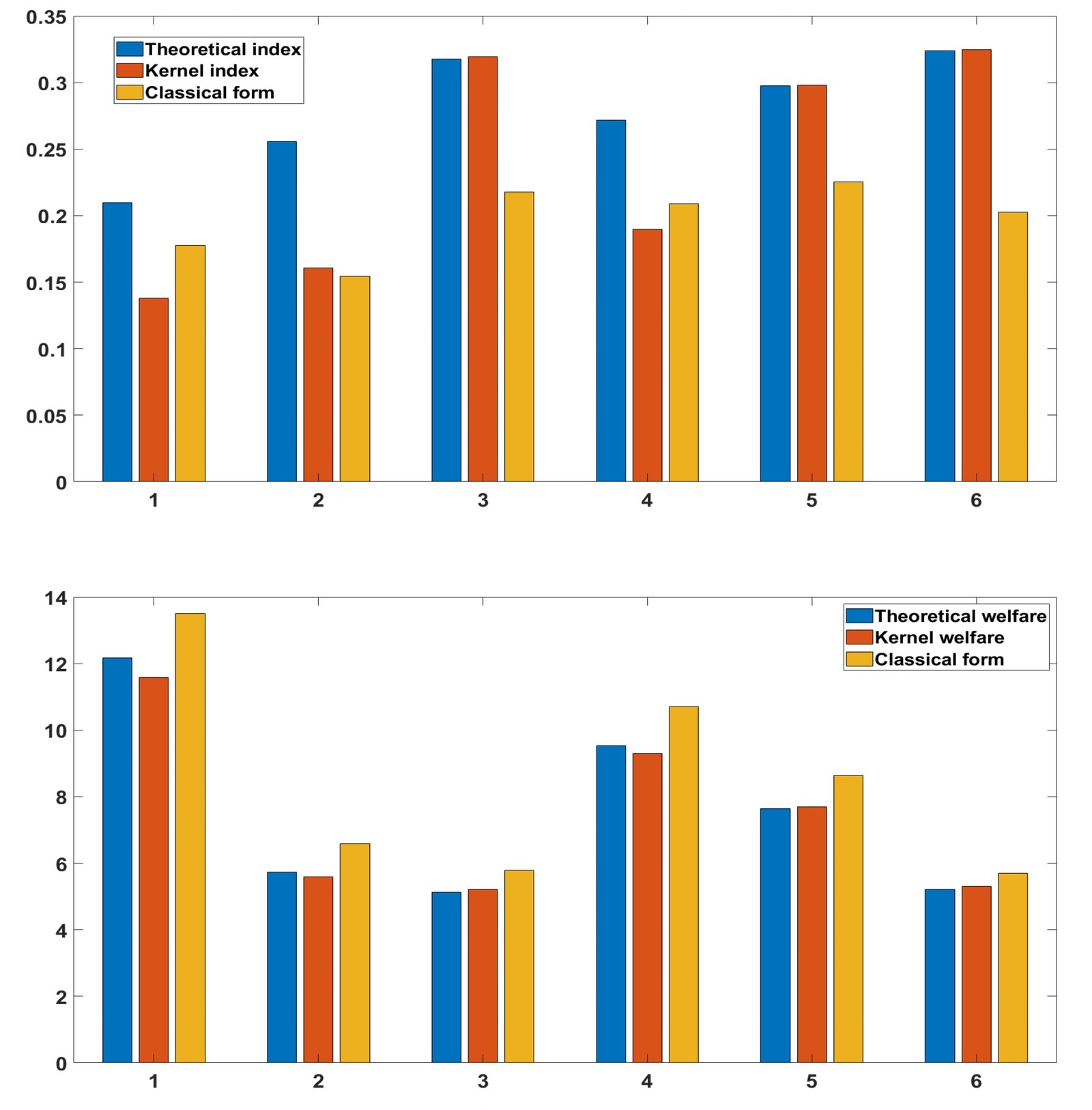
This last figure shows that the Atkinson index whatever the type of estimator does not exceed 0.35 in each zone and therefore on each continent. Although these averages do not allow us to conclude effectively or to draw an efficient objective conclusion, nevertheless they allow us to have more or less or approximately an overall view of the trend of the Atkinson indices and the values of the associated welfare in each region or zone.
On the one hand, we therefore conclude that Figure 2 and Table 3 have provided us with the behavior of our estimators in relation to the progressive choice of the aversion parameter θ. On the other hand, to estimate the Atkinson indices and the values of social welfare, it is therefore essential to find an estimator of the parameter θ or therefore find the corresponding value of θ for each data or observation. Thus we therefore propose here to find the value of θ for each of our observations. To do this, the function Φ (32) therefore becomes a bivariate function whose variables are the bandwidth and aversion parameters. The optimization problem (33) is therefore a bivariate optimization problem on the unit square surface and becomes:
\[ (\hat{h}_n, \hat{\theta}_n) = \arg \min_{h_n,\theta \in [0,1]} \Phi(h_n, \theta). \tag{34} \]Let θ̂1n and θ̂2n be the respective aversion parameters of the Atkinson index and welfare. The only parameters that do not change compared to the previous results are the parameters α̂ and β̂ from the M.L method. The results obtained are grouped in Table 4, giving the values of the Atkinson indices and those of welfare after estimating the aversion parameters. Since the classical Atkinson indices and associated welfare function do not provide a very good fit, we no longer present it in this table.
| Area or Zone | ĥ1n | θ̂1n | RMSE1 | Ân(θ) | A(θ) | ĥ2n | θ̂2n | RMSE2 | ŵn(θ) | W(θ) |
|---|---|---|---|---|---|---|---|---|---|---|
| Europe | 0.4495 | 1.0000 | 0.0127 | 0.2849 | 0.2981 | 0.9604 | 0.0851 | 0.0759 | 2.8120 | 2.8233 |
| America | 0.6547 | 0.5329 | 1.79e-10 | 0.1820 | 0.1820 | 0.8788 | 0.1152 | 3.07e-13 | 2.8195 | 2.8195 |
| Asia | 0.5710 | 0.7049 | 7.42e-08 | 0.1415 | 0.1415 | 0.8366 | 0.1142 | 2.13e-09 | 2.9905 | 2.9905 |
| Africa | 0.3894 | 0.6457 | 0.0018 | 0.2606 | 0.2606 | 0.7104 | 0.0987 | 0.0042 | 1.9499 | 1.9499 |
| Eurasia | 0.5571 | 0.9362 | 2.33e-11 | 0.2353 | 0.2353 | 0.9286 | 0.0987 | 3.71e-07 | 5.2194 | 5.2194 |
| World | 0.5306 | 0.4209 | 1.05e-07 | 0.2604 | 0.2604 | 0.7792 | 0.0939 | 5.66e-12 | 7.5482 | 7.5482 |
Table 4 allows us to draw a relatively effective conclusion as it reflects the true trends of the Atkinson index. However, we observe that in each region, the aversion parameter averages around 0.5 for the Atkinson index, except for the European region. This could be explained by the small sample size, which is less than 50. Conversely, for larger samples, the aversion parameter is lower. Regarding welfare, the aversion parameter averages 0.3. This diversity in the values of the aversion parameter once again highlights the importance of its estimation, as it has a significant influence on the estimators. Thus, compared to previous results (where θ was taken arbitrarily), we see a slight significant difference, as the indices in this case are around 0.35 or even exceed it. However, it is noteworthy that inequality is more pronounced in the Americas than in other continents. This may be due to the per capita income in North America, which is more than ten times higher than that of countries in the South or the Caribbean. In Africa and Europe, this inequality is almost identical to that of the world. Inequality is less reduced in Asia, which could be explained by the nearly identical per capita income of several countries in the Gulf and the Pacific. Overall, the disparity is significant across all continents, and world leaders must make greater efforts to raise the level of net national income per capita so that the inequality index in each continent or even in each country is at least higher than 0.7, by making appropriate decisions for the development of each country.