With the establishment of 200-mile territorial zone in the Bay of Bengal for most countries having coastlines. The control of fishing in these zones has become highly regulated by these countries concerned. In this sense, fishing in territorial waters can be considered a sole owner fishery problem. If the people of a country are allowed to fish freely in the territorial zones, it can be termed as an open access fishery. In an open access fishery, the exploitation of fishing opportunity is completely uncontrolled. This study deals with the problem of harvesting in the prey-predator fishery model in the open access zones and seeks a plan for prey for sustainable fishing, particularly in Sundarbans ecosystem which is situated in the coastal area of the Bay of Bengal. The positive steady state of both local and global stability has been established. Optimal harvesting strategy is also studied for these purposes.
This study analyzes fishery management in contest of an endangered predator population competing with human being for commercially important prey. In earlier studies, natural predators were implicitly incorporated in the fishery model. We, however, explicitly model the predator-prey relationship thinking that endangered predators can also be found in many fisheries where the expansion of the predator population and the rate of harvesting are necessary. Traditionally it is impossible to control the predator population when they are endangered. We focus on harvesting control effort over the habitat of preys for maintaining the predator-prey relationship and protected the economic importance of the fishery.
Brauer et al. in [1] and Myerscough et al. in [2] studied a general model of prey-predator interaction under constant harvesting and developed the dynamics model of harvesting. Dai et al. in [3] gave complete mathematical analysis of a prey-predator model with Holling Type I predator response Holling, [4], where both the interacting species are independently harvested. Azar et al. [5] made a comparative study between constant catch and constant harvesting effort in a prey-predator model and examined a few significant phenomena such as a constant catch on the predator may destabilize a system that is stable when a constant harvesting effort is applied. Recently, Kar et al. [6] presented a mathematical model of non selective harvesting model in a prey-predator fishery. In their work [7] they have described taxation as a control tool in their model.
Extensive and unregulated harvest of marine fishes can lead to the depletion of several fish species. Several fish species can be depleted by irrational and un regulated harvesting of marine fishes. A possible solution to these problems is to create of marine reserves restricting fishing and other related activities. This study is the modified model of Dubey et al. [8] and to analyze the optimal harvesting policy.
2. Mathematical model formulation
In a two-patch environment, we consider the following predator-prey system:
Here \(x(t),y(t)\) represents the prey population in the i-th patch, at time \(t \le 0\). We consider, the patches with a barrier only as far as the prey population is concerned and the predator population has no barriers. Thus, the total predator population for both patches is \(z(t)\). The constitutes of Patch 2, a reserve area for the prey and fishing is not allowed in this zone, though Patch 1 is an open-access fishery zone. We assumed that the prey populations are migrated randomly between two patches. In the absence of predator population, the growth rate of prey population logistically. Description of state variables and parameters is given in Table 1.
Table 1. Description of state variables and parameters.
Parameter
Description
\(r_1\) and \(r_2 \)
Intrinsic growth rates prey in the unreserved and reserved area
\(k_1\) and \(k_2\)
Environmental carrying capacity unreserved and reserved area respectively
\(\epsilon\)
dispersal rate
\(E\) and \(q \)
Harvesting effort and catchability coefficient
\(\gamma\) and \(\delta_3\)
Predator death rate and intra specific competition coefficients
If \(\epsilon = 0\), then no member of the prey population can leave its patch. From the j-th patch to the i-th patch the net exchange is proportional to the difference \(x\sim y\) of fish population densities in each patch.
3. Preliminary results
3.1. Boundedness
Now easily we can show that all solutions of system (1) -(3) are uniformly bounded.
Theorem 1.
All the solutions \((x(t),y(t),z(t))\) of the system (1) -(3) in \(\mathbb{R}_+^3\) are bounded.
Proof.
To prove the theorem, we consider the following function $$w(t)=\frac{c_1}{\alpha_1}x(t)+\frac{c_2}{\alpha_2}y(t)+z.$$
Therefore, time derivative is found to be
It is clear that the right-hand side of inequality (5) is bounded for all \((x,y,z)\in\Re_+^3\), provide \(E\) is bounded.
Therefore, we take \(v>0\) such that $$\frac{dw}{dt}+\mu w\le v.$$
Using the theory of differential inequalities developed by Birkhoff et al. in [9] we obtain,
Theorem 2.
If \( r_2\ge\epsilon\) then the system (1) -(3) is dissipative.
Proof.
By usual straight forward arguments, we can show that the solution of the system (1) -(3) always exists and is positive, In fact from the Equations
(1) -(3) of the model system that \(lim_{t\to\infty} x(t)\le 1\) from Equations (2) we notice that
\(\dot y=r_2y(1-\frac{y}{k_2})+\epsilon(x-y)-\alpha_2yz\le y(r_2-\epsilon).\) By similar arguments, we have, \(lim_{t\to\infty} y(t)\le(r_2-\epsilon)=\bar{y}\)
where \(\bar{y}\) denotes an upper bound of \(y(t)\) which will be positive if \(r_2>\epsilon.\)
4. Equilibria analysis
Theorem 3.
The possible steady states of the system of Equations (1) -(3) are:
Solving (10) -(12) we will find interior equilibrium point.
5. Stability analysis
5.1. local stability
Now, we investigate the local asymptotically stability of the model (1) -(3) around the feasible equilibrium points.
5.1.1. Stability for \(E_0\)
$$\lambda[\lambda^2-(r_1+r_2-2\epsilon-qE)\lambda+(r_1-qE)(r_2-\epsilon)-r_2\epsilon]=0.$$
The equilibrium point \(E_0\) is a saddle point with locally stable manifold in \(xy\)- plane and with locally unstable manifold in \(z\)-direction if $$\frac{1}{q}\left(r_1+r_2-2\epsilon\right)< E< \frac{r_1r_2-(r_1+r_2)\epsilon}{q(r_2-\epsilon)}.$$
5.1.2. Stability for \(E_1\)
The characteristic equation for \(E_1\) is given by
$$\lambda\left[\lambda^2+\left\{\frac{r_1x}{k_1}+\frac{r_2y}{k_2}+\epsilon\big(\frac{x}{y}+\frac{y}{x}\big)\right\}\lambda+\frac{r_1x}{k_1}\left(\frac{r_2y}{k_2}+\epsilon\frac{x}{y}\right)+\frac{r_2y^2}{xK_2}\right]=0.$$
Therefore, \(E_1\) is a saddle point with locally stable manifold in \(xy\)- plane and with locally unstable manifold in the \(z\)-direction.
5.1.3. Stability for \(E_2\)
The characteristic equation for \(E_2\) is given by
where,
\begin{align*}
a&=\frac{r_1x^*}{k_1}+\frac{r_2y^*}{k_2}+\epsilon\left(\frac{y^*}{x^*}+\frac{x^*}{y^*}\right)+z^*\delta>0\\
b&=y^*\delta(\alpha-z^*\delta)+\frac{r_2y^*}{k_2}\left(\frac{r_1x^*}{k_1}+\frac{\epsilon y^*}{x^*}\right)+(\alpha_1c_1x^*+\alpha_2c_2y^*)z^*+\frac{\epsilon r_1x^{*2}}{k_1y^*}>0\\
c&=z^*\left[y^*\left(\frac{r_1x^*}{k_1}+\frac{\epsilon y^*}{x^*}\right)+\left(\frac{r_2\delta}{k_2}+\alpha_2c_2\right)+c_1\alpha_1x^*\left(\frac{r_2x^*}{k_2}+\frac{\epsilon y^*}{x^*}\right)+\frac{\epsilon r_1\delta x^{*2}}{k_1y^*}+\epsilon(\alpha_2c_1y^*+\alpha_1c_2x^*)\right]>0.
\end{align*}
We see that all eigenvalues of Equation (13) have negative real parts if and only if \(a>0, \quad c>0\) and \(ab-c>0\) which satisfies the Routh-Hurwitz criterion. Here, \(a>0, \quad c>0\) and it is easy to examined that \(ab-c>0\). Hence, \(E^*(x^*,y^*,z^*)\) is locally asymptotically stable.
5.2. Global stability analysis
From the point of view of ecological managers it may be found an equilibrium point where the model system is globally asymptotically stable in order to plan harvesting strategy and keep sustainable ecological development. Therefore, in the interior equilibrium point \(E^*(x^*,y^*,z^*)\), we have discussed the global stability.
Theorem 4.
The model system (1) -(3) is globally asymptotically stable in the positive equilibrium point \(E^*(x^*,y^*,z^*)\) if \(\epsilon\big(\sqrt{\frac{\sigma_1}{x^*}}-\sqrt{\frac{\sigma_2}{y^*}}\big)^2< 2\sqrt{\sigma_1\sigma_2\frac{r_1r_2}{k_1k_2}}.\)
Proof.
Using the standard Lyapunov function we have,
Along a solution, the derivative of (1) -(3) takes the form:
\begin{align*}
\dot V&=\sigma_1(x-x^*)\left(r_1-\frac{r_1}{k_1}x-\alpha_1z+E\frac{y-x}{x}\right)+\sigma_2(y-y^*)\left(r_2-\frac{r_2}{k_2}y-\alpha_2z+\epsilon\frac{x-y}{y}\right)\\
&\,\,\,\,+\sigma_3(z-z^*)(-\gamma-\delta z+c_1x+c_2y)\\
&=-\sigma_1\frac{r_1}{k_1}\left(x-x^*\right)^2+\sigma_2(y-y^*)^2-(z-z^*)\{\sigma_1\alpha_1(x-x^*)+\sigma_2\alpha_2(y-y^*)\}\\
&\,\,\,\,-\sigma_3\delta(y-y^*)\{c_1(x-x^*)+c_2(y-y^*)\}-\epsilon\Gamma(x,y),
\end{align*}
where $$\Gamma(x,y)=\sigma_1y\frac{(x-x^*)}{xx^*}+\sigma_2x\frac{(y-y^*)}{yy^*}-\big(\frac{\sigma_1}{x}+\frac{\sigma_2}{y}\big)(x-x^*)(y-y^*)$$
If we choose \(\sigma_1=\frac{c_1}{\alpha_1}\quad\sigma_2=\frac{c_2}{\alpha_2},\quad\sigma_3=1\), then we have $$\dot V=-\sigma_1\frac{r_1}{k_1}(x-x^*)^2+\sigma_2\frac{r_2}{k_2}(y-y^*)^2-\delta(z-z^*)^2-\epsilon\Gamma(x,y).$$
Now it is easy to show that
$$\Gamma(x,y)\ge \left(2\sqrt{\frac{\sigma_1\sigma_2}{x^*y^*}}-\frac{\sigma_1}{x^*}-\frac{\sigma_2}{y^*}\right)(x-x^*)(y-y^*)
=-\left(\sqrt{\frac{\sigma_1}{x^*}}-\sqrt{\frac{\sigma_2}{y^*}}\right)^2(x-x^*)(y-y^*).$$
Thus we have, $$\dot V=-\sigma_1\frac{r_1}{k_1}(x-x^*)^2+\sigma_2(y-y^*)^2-\delta(z-z^*)^2-\epsilon\left(\sqrt{\frac{\sigma_1}{x^*}}-\sqrt{\frac{\sigma_2}{y^*}}\right)^2(x-x^*)(y-y^*).$$
Therefore \(\epsilon\left(\sqrt{\frac{\sigma_1}{x^*}}-\sqrt{\frac{\sigma_2}{y^*}}\right)^20\) and \((x,y,z)\ne (x^*,y^*,z^*),\quad \dot V< 0\). Therefore, we say that, \(E^*(x^*,y^*,z^*)\) is globally asymptotically stable.
6. Bionomic equilibrium and and optimal harvesting policy
The bionomic equilibrium is said to be achieved when the total revenue is earned by the difference of pricing and harvesting cost. Let us consider the constant fishing cost per unit effort is \(c\) and the constant price per unit landed fish in the open access area is \(p\). Therefore, the economic rent is given as follows
Now, if \(c>pqx\), i.e., if the fishing cost exceeds the revenue, then the economic rent obtained from the fishery becomes negative and the fishery will be closed. Therefore, the bionomic equilibrium existence, it is assumed that \(c>pqx\). The positive bionomic equilibrium solutions of \(\dot x=\dot y=\dot z=\Pi=0\) is \((x_\infty,y_\infty,z_\infty,E_\infty).\) Solving these equations we get,
$$x_\infty=\frac{c}{pq}$$
$$y_\infty=\frac{\left[\alpha_2\left(-\gamma+\frac{cc_1}{pq}\right)+\delta(\epsilon-r_2)\right]+\sqrt{\left[\alpha_2(-\gamma+\frac{cc_1}{pq}+\delta(\epsilon-r_2))^2+\frac{4r_2\epsilon c}{pq}(\alpha_2c_2+\frac{\delta r_2}{k_2})\right]}}{2(\alpha_2c_2+\frac{\delta r_2}{k_2})}$$
$$z_\infty=\frac{1}{\delta}\left(-\gamma+\frac{cc_1}{pq}+c_2y_\infty\right)$$
and $$E_\infty=\frac{1}{\delta}\left[r_1\left(1-\frac{c}{k_1pq}\right)-\epsilon-\frac{\alpha_1}{\delta}\left(-\gamma+\frac{cc_1}{pq}\right)+\left(\frac{\epsilon pq}{c}-\frac{\alpha_1c_2}{\delta}\right)y_{\infty}\right].$$
If \(E>E_\infty\) , then the total harvesting cost the fish population will exceed the total amount of revenues collected from the fishery. Therefore, we assumed that some fishermen will face loss and withdraw themselves from fishing. Hence \(E>E_\infty\) is possible to be maintained indefinitely. The fishery is more profitable when \(\frac{d\lambda_1}{dt}=-\frac{\partial H}{\partial x}\) and hence in an open access fishery it would be attracted more and more fishermen which increasing the harvesting. Hence \(E< E_\infty\) is not possible to maintain indefinitely.
Now our objective is to maximizes the present value of a continuous time-stream of revenues. We select a harvesting strategy. Consider \(\sigma\) be the instantaneous annual discount rate,
The problem (16), subject to the Equations (1)-(3), by applying Pontryagin’s maximum Principle with control constant \(0< E< E_{max}\) can be solved. The feasible upper limit on the harvesting effort \(E_{max}\). Then the Hamiltonian problem is given by
where \(\lambda_1,\quad\lambda_2\) and \(\lambda_3\) are adjoint variables and \(\mu(t)=(e_{\sigma t}(pqx-c)E)-\lambda_1qx\) is called the switching function. The optimal control \(E(t)\) the maximizes the linear control variable of Hamiltonian \(H\) must satisfying conditions:
\(E=E_{max}\) when \(\mu(t)>0\) i.e., when \(\lambda_1(t)e^{\sigma t}< p-\frac{c}{qx};\)
\(E=0\) when \(\mu(t)p-\frac{c}{qx};\)
\(\lambda_1(t)e^{\sigma t}\) is the traditional shadow price and p-is the net economic revenue on a unit harvest which shows that \(E=E_{max}\) according as the shadow price is less than or greater than the net economic revenue on a unit harvest. Economically, the first condition is that after passing all the expenses if the profit is positive, then it is beneficial to harvest up to the limit of available effort and second condition is that when the shadow price exceeds the fishermen’s net economic revenue on a unit harvest, then the fishermen will not exert any effort. When \(\mu(t)=0\) , i.e., when the shadow price on a unit harvest equals the net economic revenue, then the Hamiltonian \(H\) of the control variable \(E(t)\) i.e., \(\frac{\partial H}{\partial E}=0\) becomes independent. It is the necessary condition to be optimal over the control set \(0< E^*< E_{max}\) for the singular control \(E^*(t)\). Thus the optimal harvesting policy is
This implies at the steady state effort level, the total user harvesting cost per unit effort must be equal to the discounted value of the future profit.
Now, we have the adjoint equations as follows:
\begin{eqnarray}
&&\frac{d\lambda_1}{dt}=-\frac{\partial H}{\partial x}=-\left[pqEe^{\sigma t}+\lambda_1\{r_1\left(1-\frac{2x}{k_1}\right)-\epsilon-\alpha_1z-qE\}+\lambda_2\epsilon+\lambda_3zc_1\right]\nonumber\\
&&\frac{d\lambda_2}{dt}=-\frac{\partial H}{\partial y}=-\left[\lambda_1\epsilon+\lambda_2\{r_2\left(1-\frac{2y}{k_2}\right)-\epsilon-\alpha_2y\}+\lambda_3zc_2\right]\nonumber\\
&&\frac{d\lambda_3}{dt}=-\frac{\partial H}{\partial z}=-[-\lambda_1\alpha_1y-\lambda_2\alpha_2y-\lambda_3\delta z].\nonumber
\end{eqnarray}
Here \(x,y,z\) and \(E\) can be treated as constants to find optimal equilibrium solution of the system. Therefore, adjoint equations are given as follows:
Now from Equations (21),(22) and (23) eliminating \(\lambda_2\) and \(\lambda_3\) we get
\(D^3-[\frac{r_1x}{k_1}+\frac{r_2y}{k_2}+\epsilon(\frac{x}{y}+\frac{y}{x})+\delta z]D^2+[\big(\frac{r_2y}{k_2}+\epsilon\frac{x}{y}+\delta z\big)\{\frac{r_1x}{k_1}+\epsilon(\frac{y}{x}+\frac{c_1}{c_2})\}+\{\delta(\frac{r_2y}{k_2}+\epsilon\frac{x}{y})\}+\alpha_1c_1x+\alpha_2c_2y-\epsilon\delta\frac{c_1}{c_2}\}z-\epsilon\frac{c_1}{c_2}(\frac{r_2y}{k_2}+\epsilon\frac{x}{y})-\epsilon^2]D-[\{\delta z(\frac{r_2y}{k_2}+\epsilon\frac{x}{y})+\alpha_2c_2yz\}\{\frac{r_1x}{k_1}+\epsilon(\frac{y}{x}+\frac{c_1}{c_2})\}+\{\frac{c_1}{c_2}(\frac{r_2y}{k_2}+\epsilon\frac{x}{y})+\epsilon\}(\alpha_1c_2x-\epsilon\delta)z]=Me^{\sigma t},\)
where \(M=-pqE[\sigma^2+\sigma(\frac{r_2y}{k_2}+\epsilon\frac{x}{y})(1+y)+(\delta^2+\alpha_2c_2y)z]\). The auxiliary equation is
\(m^3-[\frac{r_1x}{k_1}+\frac{r_2y}{k_2}+\epsilon(\frac{x}{y}+\frac{y}{x})+\delta z]m^2+[\big(\frac{r_2y}{k_2}+\epsilon\frac{x}{y}+\delta z\big)\{\frac{r_1x}{k_1}+\epsilon(\frac{y}{x}+\frac{c_1}{c_2})\}+\{\delta(\frac{r_2y}{k_2}+\epsilon\frac{x}{y})\}+\alpha_1c_1x+\alpha_2c_2y-\epsilon\delta\frac{c_1}{c_2}\}z-\epsilon\frac{c_1}{c_2}(\frac{r_2y}{k_2}+\epsilon\frac{x}{y})-\epsilon^2]m-[\{\delta z(\frac{r_2y}{k_2}+\epsilon\frac{x}{y})+\alpha_2c_2yz\}\{\frac{r_1x}{k_1}+\epsilon(\frac{y}{x}+\frac{c_1}{c_2})\}+\{\frac{c_1}{c_2}(\frac{r_2y}{k_2}+\epsilon\}\frac{x}{y})+\epsilon(\alpha_1c_2x-\epsilon\delta)z]=0.\nonumber
\)
Consider the root of the above equation are \(m_1, m_1\) and \(m_3\), then the general solution becomes \(\lambda_1(t)=A_1e^{m_1t}+A_2e^{m_2t}+A_3e^{m_3t}+\frac{M}{N}e^{-\sigma t},\) where
\(N=-\sigma^3-[\frac{r_1x}{k_1}+\frac{r_2y}{k_2}+\epsilon(\frac{x}{y}+\frac{y}{x})+\delta z]\sigma^2+[\big(\frac{r_2y}{k_2}+\epsilon(\frac{x}{y}+\delta z\big)\{\frac{r_1x}{k_1}+\epsilon(\frac{y}{x}+\frac{c_1}{c_2})\}+\{\delta(\frac{r_2y}{k_2}+\epsilon\frac{x}{y})\}+\alpha_1c_1x+\alpha_2c_2y-\epsilon\delta\frac{c_1}{c_2}\}z-\epsilon\frac{c_1}{c_2}(\frac{r_2y}{k_2}+\epsilon\frac{x}{y})-\epsilon^2]\sigma-[\{\delta z(\frac{r_2y}{k_2}+\epsilon\frac{x}{y})+\alpha_2c_2yz\}\{\frac{r_1x}{k_1}+\epsilon(\frac{y}{x}+\frac{c_1}{c_2})\}+\{\frac{c_1}{c_2}(\frac{r_2y}{k_2}+\epsilon\frac{x}{y})+\epsilon\}(\alpha_1c_2x-\epsilon\delta)z]\ne 0.\)
The shadow price \(\lambda_1(t)e^{\sigma t}\) remains bounded as \(t\to \infty\) if and only if \(A_1=A_2=A_3=0\) and then \(\lambda_1(t)e^{\sigma t}=\frac{M}{N}=\text{constant.}\)
Now substituting \(\lambda_1(t)\) in (19) we get,
Together with equation \(\dot x=\dot y=\dot z=0\) and Equation (23), gives the optimal equilibrium populations \(x=x_\infty, y=y_\infty\) and \(z=z_\infty,\)
when \(\sigma\to\infty,\) Equation (23) leads to obvious result \(pqx_\infty=c\) that implies \(\Pi(x_{\infty},y_{\infty},z_{\infty}, E_{\infty})=0.\)
This shows that infinite discount rate leads to a economic revenue which is completely dissipation. Using (23), we have \(\Pi=(pqx-c)E=\frac{MqxE}{N}\).
Since \(M\) is of \(O{(\sigma)}\) where \(N\) is \(O(\sigma^2)\) we see that \(\Pi\) is \(O(\sigma^{-1}\). Thus, the decreasing function of \(\sigma(\le 0)\) is \(\Pi\). Therefore, we conclude that \(\sigma=0\) leads to maximization of \(\Pi.\)
7. Numerical simulation
Analytical studies can never be completed without numerical verification of the derived results. In this section, we present computer simulations of some solutions of the system (1) -(3). Beside verification of our analytical findings, these numerical simulations are very important from practical point of view. We use four different set of numerical values for support of analytical results mentioned in Table 2.
Table 2. Set of parameter values for numerical simulations; \(S\equiv \)Parameter sets.
\(r_1\)
\(r_2\)
\(k_1\)
\(k_2\)
\(\epsilon\)
\(\alpha_1\)
\(\alpha_2\)
\(\gamma_1\)
\(\delta\)
\(c_1\)
\(c_2\)
\(E\)
\(q\)
\(3\)
\(1.5\)
\(50\)
\(40\)
\(0.5\)
\(0.2\)
\(0.2\)
\(0.6\)
\(0.05\)
\(0.03\)
\(0.04\)
\(2\)
\(0.01\)
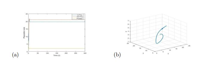
From the theory established earlier the interior equilibrium point \(E_2(19.50, 10.20, 7.86)\) is globally asymptotically stable. From the Figure 1, we may conclude that the steady state \(E_2(19.50, 10.20, 7.86)\) is globally asymptotically stable. Hence the theory established earlier is verified.
Figure 1. Stability behaviour of model the system around the equilibrium position \(E_*\) with the initial conditions and the set of parameter values \(S\),
(a) Time series (b) Phase portrait.
8. conclusion
This research deals with the harvesting problem in a prey-predator fishery model the reserved zone for prey species in the Sundarban. The positive steady state of both local and global stability has been established. To get global stability, it is necessary that the dispersal rate to be bounded above by related constant. In the exploited model system, we have examined the possibilities of the existence of bionomic equilibria. By using Pontryagin’s maximum principle, we have optimized the harvesting policy. We have found that the shadow prices satisfy the transversality condition when they are constant. The total user cost of harvest per unit effort is equal to the steady state effort. We have shown that zero discounting maximizes the economic revenue and that an infinite discount rate is completely dissipate.
Author Contributions
All authors contributed equally to the writing of this paper. All authors read and approved the
final manuscript.
Competing Interests
The author(s) do not have any competing interests in the manuscript.
References
Brauer, F., & Soudack, A. C. (1982). Coexistence properties of some predator-prey systems under constant rate harvesting and stocking. Journal of Mathematical Biology, 12(1), 101-114.[Google Scholor]
Myerscough, M. R., Gray, B. F., Hogarth, W. L., & Norbury, J. (1992). An analysis of an ordinary differential equation model for a two-species predator-prey system with harvesting and stocking. Journal of Mathematical Biology, 30(4), 389-411. [Google Scholor]
Dai, G., & Tang, M. (1998). Coexistence region and global dynamics of a harvested predator-prey system. SIAM Journal on Applied Mathematics, 58(1), 193-210. [Google Scholor]
Holling, C. S. (1965). The functional response of predators to prey density and its role in mimicry and population regulation. The Memoirs of the Entomological Society of Canada, 97(S45), 5-60. [Google Scholor]
Azar, C., Holmberg, J., & Lindgren, K. (1995). Stability analysis of harvesting in a predator-prey model. Journal of Theoretical Biology, 174(1), 13-19. [Google Scholor]
Kar, T. K., & Chaudhuri, K. S. (2002). On non-selective harvesting of a multispecies fishery. International Journal of Mathematical Education in Science and Technology, 33(4), 543-556. [Google Scholor]
Kar, T. K., & Chaudhuri, K. S. (2003). On non-selective harvesting of two competing fish species in the presence of toxicity. Ecological Modelling, 161(1-2), 125-137.[Google Scholor]
Dubey, B., Chandra, P., & Sinha, P. (2003). A model for fishery resource with reserve area. Nonlinear Analysis: Real World Applications, 4(4), 625-637. [Google Scholor]
Birkhoff, G., & Rota, G. C. (1982). Ordinary Differential Equations. 1989. Ginn, Boston.[Google Scholor]