
Nonlinear parabolic equations of \(p\)–Laplace type arise naturally in a wide range of scientific and engineering applications, including non–Newtonian fluid flows, nonlinear heat conduction, porous media diffusion, material science, and biological transport processes. A prototypical model is given by \[\label{equation.1} \partial_t u – \nabla \cdot \bigl( |\nabla u|^{p-2} \nabla u \bigr) = f, \tag{1}\] which generalizes the classical heat equation corresponding to the linear case \(p=2\).
The mathematical analysis of such equations has a long and well–established history. Early foundational contributions were made by Ladyzhenskaya and Uraltseva in their seminal works on degenerate and singular elliptic and parabolic equations in the 1960s [1]. A systematic treatment of degenerate parabolic equations, including regularity properties and intrinsic scaling techniques, was later developed by DiBenedetto [2]. Depending on the exponent \(p\), the diffusion operator exhibits either degenerate behavior for \(1<p<2\) or singular behavior for \(p>2\), which typically leads to limited regularity of weak solutions and the formation of steep gradients or free–boundary–type phenomena.
From the perspective of nonlinear functional analysis, the theory of weak solutions to nonlinear evolution equations is deeply rooted in the framework of monotone operators and Sobolev spaces. Fundamental results on existence, uniqueness, and stability of solutions were established by Lions [3], Showalter [4], and Zeidler [5]. These works provide the analytical foundation for parabolic problems involving the \(p\)–Laplace operator, ensuring well–posedness under minimal regularity assumptions on the data.
On the numerical side, the finite element method has become one of the most powerful tools for the approximation of partial differential equations. The concept of a posteriori error estimation and adaptive mesh refinement was pioneered by Babuška and Rheinboldt [6, 7], and later systematically developed by Verfürth [8, 9] for linear elliptic and parabolic problems. Adaptive finite element methods (AFEM) are particularly attractive for problems with localized phenomena, as they allow the computational effort to be concentrated in regions where the solution exhibits large gradients or reduced regularity.
For nonlinear problems, substantial progress has been made in recent years for the elliptic \(p\)–Laplace equation. Convergence and optimality results for adaptive schemes have been obtained, for instance, in [10– 12]. In contrast, the parabolic \(p\)–Laplace problem has been studied predominantly within time–stepping frameworks, where the spatial discretization and the temporal integration are treated separately. While such approaches are effective for sufficiently smooth solutions, they are often less suitable for capturing strong space–time interactions or highly nonuniform temporal behavior.
Fully spacetime finite element methods offer an appealing alternative by treating space and time within a unified variational framework. For linear parabolic and hyperbolic problems, spacetime discretizations have been shown to provide enhanced stability, flexibility, and parallelization capabilities; see, for example, the works of Steinbach, Moore, and Langer [13– 15]. However, systematic investigations of adaptive spacetime finite element methods for nonlinear parabolic equations of \(p\)–Laplace type, including rigorous a posteriori error control and convergence analysis, are still largely unexplored.
The purpose of this paper is to address this gap. We develop and analyze an adaptive spacetime finite element method for nonlinear parabolic equations of \(p\)–Laplace type. Our approach combines a unified spacetime variational formulation with residual–based a posteriori error estimators, allowing for simultaneous mesh refinement in space and time. We establish well–posedness of the discrete problem, discrete energy stability, reliability and efficiency of the error estimator, and convergence of the adaptive scheme under minimal regularity assumptions. Numerical experiments are presented to illustrate the theoretical results and to demonstrate the advantages of spacetime adaptivity over uniform and time–stepping approaches.
Nonlinear parabolic equations of \(p\)-Laplace type arise naturally in a wide range of scientific and engineering applications, where diffusion or transport processes depend nonlinearly on the gradient of the unknown solution. A prototypical model is the parabolic \(p\)-Laplace Eq. (1) which can be viewed as a nonlinear generalization of the classical heat equation corresponding to the linear case \(p=2\).
An important application of such equations appears in the modeling of non-Newtonian fluid flows, where the viscosity of the fluid depends on the rate of deformation. In these models, the velocity field satisfies a parabolic equation involving a \(p\)-Laplace type operator, with the parameter \(p\) characterizing shear-thinning behavior \((1<p<2)\) or shear-thickening behavior \((p>2)\). These models play a fundamental role in the description of polymeric fluids, suspensions, and various biological fluids.
Another significant class of applications concerns nonlinear diffusion processes, including flow in porous media, population dynamics, and image processing. In such problems, the diffusion coefficient reflects heterogeneous or concentration-dependent transport mechanisms, which naturally lead to \(p\)-Laplace type operators. Similarly, nonlinear heat conduction in materials with temperature-dependent thermal conductivity can be described by parabolic equations with nonlinear diffusion terms.
In continuum mechanics and material science, equations of \(p\)-Laplace type are employed to model viscoplasticity, damage evolution, and strain localization phenomena. Moreover, in biological applications, such equations arise in models of cell migration, chemotaxis, and tissue growth, where diffusion processes are inherently nonlinear and anisotropic.
Despite their broad applicability, the numerical approximation of nonlinear parabolic equations of \(p\)-Laplace type remains challenging. Classical finite element methods typically rely on a separation of space and time discretizations, for instance by combining spatial finite elements with time-stepping schemes. While effective for smooth solutions, such approaches often struggle to accurately capture phenomena with strong space–time coupling, moving fronts, or localized features.
Furthermore, the use of uniform meshes in both space and time is generally inefficient for problems exhibiting degenerate or singular solutions, which are characteristic of \(p\)-Laplace equations. In such cases, computational resources are wasted in regions where the solution is smooth, while critical regions with steep gradients or rapid temporal variations remain under-resolved.
These limitations motivate the development of spacetime finite element methods, in which space and time are treated within a unified variational framework. By discretizing the entire spacetime domain simultaneously, spacetime methods are able to capture complex space–time interactions more effectively and allow for flexible local refinement. When combined with adaptive strategies, enabling refinement in both space and time based on rigorous error indicators, this approach provides a powerful and efficient framework for the numerical approximation of nonlinear parabolic problems with evolving solution features.
The analysis and numerical approximation of parabolic equations of \(p\)-Laplace type involve several intrinsic mathematical difficulties. The primary challenge arises from the strong nonlinearity of the diffusion operator \[\label{equation.2} \nabla \cdot \left( |\nabla u|^{p-2} \nabla u \right), \tag{2}\] which is neither linear nor uniformly elliptic except in the case \(p=2\). Although the operator is monotone and coercive, its behavior depends strongly on the value of \(p\).
For \(1<p<2\), the operator becomes degenerate, leading to reduced diffusion in regions where \(|\nabla u|\) is small. This degeneracy may result in limited regularity of the solution and the formation of sharp gradients or free boundaries. In contrast, for \(p>2\), the operator is singular, exhibiting enhanced diffusion for large gradients, which complicates both stability analysis and numerical error control.
In addition to spatial difficulties, solutions of nonlinear parabolic equations often exhibit non-uniform temporal behavior, such as rapid initial transients followed by slow evolution. Accurately capturing these phenomena requires discretization techniques that adapt simultaneously in space and time. Fixed time-step methods may therefore be inefficient or insufficiently accurate.
From an analytical point of view, these challenges manifest themselves in the limited regularity of weak solutions, the absence of superposition principles, and the difficulty of deriving optimal a priori error estimates. Consequently, any reliable numerical method must be carefully designed to respect the nonlinear structure of the problem while guaranteeing stability and convergence under minimal regularity assumptions.
Finite element approximations of \(p\)-Laplace type problems have been widely studied in the literature. For the elliptic \(p\)-Laplace equation, convergence and stability results are well established, typically based on monotone operator theory and nonlinear approximation techniques.
In the parabolic case, most existing works focus on time-discrete or semi-discrete methods, combining implicit time-stepping schemes with spatial finite elements. While these approaches provide solid theoretical foundations, they inherently separate space and time and therefore do not fully exploit spacetime adaptivity.
Spacetime finite element methods have been developed mainly for linear parabolic and hyperbolic problems. Notable contributions by Steinbach, Andreev, and Langer have demonstrated the advantages of spacetime formulations in terms of stability, flexibility, and parallel efficiency. However, the majority of these results are restricted to linear or mildly nonlinear equations.
Adaptive finite element methods based on a posteriori error estimation have also been extensively investigated, especially for elliptic problems and linear parabolic equations. Nevertheless, rigorous results for adaptive spacetime finite element methods applied to nonlinear parabolic equations of \(p\)-Laplace type remain very limited.
This paper aims to bridge the aforementioned gap by developing and analyzing an adaptive space-time finite element method for p-Laplace type nonlinear parabolic equations.
The structure of this paper is as follows:
1. Introduction
2. Preliminaries
3. Problem setting
4. Existence and uniqueness of weak solution
5. Adaptive spacetime finite element discretization
6. A Posteriori error estimation
7. Convergence analysis
8. Numerical experiments
9. Adaptive spacetime algorithm
In this section, we recall some basic concepts and results related to Sobolev spaces and the \(p\)-Laplacian operator.
\(L^p(\Omega)\) and \(L^{p'}(\Omega)\). For a measurable domain \(\Omega \subset \mathbb{R}^n\) and \(1 \leq p < \infty\), the Lebesgue space \(L^p(\Omega)\) is defined by \[\label{equation.3} L^p(\Omega) = \left\{ u : \Omega \to \mathbb{R} \;\bigg|\; \int_\Omega |u(x)|^p \, dx < \infty \right\}, \tag{3}\] with the norm \[\label{equation.4} \|u\|_{L^p(\Omega)} = \left( \int_\Omega |u(x)|^p \, dx \right)^{1/p}. \tag{4}\]
In the case \(p = \infty\): \[L^\infty(\Omega) = \left\{ u : \Omega \to \mathbb{R} \;\big|\; \operatorname*{ess\,sup}_{x \in \Omega} |u(x)| < \infty \right\}.\]
For \(1 < p < \infty\), the conjugate exponent \(p'\) is defined by \[p' = \frac{p}{p-1}, \qquad \frac{1}{p} + \frac{1}{p'} = 1.\]
By the duality theorem, we have \[\big(L^p(\Omega)\big)' \simeq L^{p'}(\Omega),\] with the bilinear form \[\langle u, v \rangle = \int_\Omega u(x)v(x)\, dx.\]
Let \(X\) be a Banach space with dual space \(X^*\). The natural embedding \[\iota: X \to X^{**}, \quad (\iota(x))(f) := f(x), \quad \forall f \in X^*, \tag{5}\] is injective. If \(\iota\) is also onto, that is, \[X \cong X^{**}, \tag{6}\] then \(X\) is called a reflexive Banach space.
Let \(X\) be a Banach space and \([0,T]\) a time interval. A function \[F: [0,T] \times X \to X^*,\] is called a Carathéodory function if:
(1) For each \(x \in X\), the mapping \(t \mapsto F(t,x)\) is measurable.
(2) For almost every \(t \in [0,T]\), the mapping \(x \mapsto F(t,x)\) is continuous.
In other words, a Carathéodory function combines:
(1) Continuity with respect to the spatial variable \(x\).
(2) Measurability with respect to the time variable \(t\).
Theorem 1(Cauchy-Schwarz inequality).Let \(H\) be an inner product space with inner product \(\langle \cdot, \cdot \rangle\). For any \(u, v \in H\), we have \[|\langle u, v \rangle| \le \|u\| \, \|v\|, \tag{7}\] where \(\|u\| = \sqrt{\langle u,u \rangle}\).
Theorem 2(Young’s inequality).Let \(a, b \ge 0\) and \(p, q > 1\) with \(\frac{1}{p} + \frac{1}{q} = 1\). Then \[ab \le \frac{a^p}{p} + \frac{b^q}{q}. \tag{8}\]
Theorem 3(Hölder’s inequality).Let \(1 \le p, q \le \infty\) with \(\frac{1}{p} + \frac{1}{q} = 1\). For any \(f \in L^p(\Omega)\) and \(g \in L^q(\Omega)\), we have \[\int_\Omega |f(x) g(x)| \, dx \le \|f\|_{L^p(\Omega)} \, \|g\|_{L^q(\Omega)}. \tag{9}\]
In existence theorems (e.g., the Carathéodory theorem), one often assumes a growth condition: \[\|F(t,x)\|_{X^*} \le a(t) + b \|x\|_X^{p-1}, \quad a \in L^{p'}(0,T), \; b \ge 0, \tag{10}\] where \(1 < p < \infty\) and \(p'\) is the conjugate exponent \((1/p + 1/p' = 1)\). This ensures that \(F(t,x)\) does not grow too fast and allows the use of weak compactness in reflexive Banach spaces.
Carathéodory functions often appear in evolution equations: \[u'(t) + A(u(t)) = F(t,u(t)), \quad u(0) = u_0, \tag{11}\] where \(A: X \to X^*\) is monotone, coercive, and hemicontinuous.
– They allow the application of the Galerkin method and weak convergence to prove existence of solutions.
– Well-suited to reflexive Banach spaces, since every bounded sequence has a weakly convergent subsequence.
(1) Weak compactness: Every bounded sequence \((x_n) \subset X\) has a weakly convergent subsequence \(x_{n_k} \rightharpoonup x\) in \(X\).
(2) Dual space: If \(X\) is reflexive, then its dual \(X^*\) is also reflexive.
(3) Subspaces: Every closed subspace of a reflexive Banach space is reflexive.
\(\bullet\) \(L^p(\Omega)\) is reflexive for \(1 < p < \infty\).
\(\bullet\) \(W^{1,p}(\Omega)\) is reflexive for \(1 < p < \infty\).
\(\bullet\) Non-reflexive examples: \(L^1(\Omega)\), \(L^\infty(\Omega)\).
\(W^{1,p}(\Omega)\). For \(1 < p < \infty\), the first-order Sobolev space \(W^{1,p}(\Omega)\) is defined by \[W^{1,p}(\Omega) = \left\{ u \in L^p(\Omega) : \partial_{x_i} u \in L^p(\Omega), \; i=1,\dots,n \right\},\] with the norm \[\|u\|_{W^{1,p}(\Omega)} = \Big( \|u\|_{L^p(\Omega)}^p + \|\nabla u\|_{L^p(\Omega)}^p \Big)^{1/p}.\]
The subspace \(W^{1,p}_0(\Omega)\) is defined as the closure of \(C_0^\infty(\Omega)\) with respect to the above norm.
\(W^{-1,p}(\Omega)\). We define \[W^{-1,p}(\Omega) := \big(W^{1,p'}_0(\Omega)\big)',\] that is, the dual space of \(W^{1,p'}_0(\Omega)\). An element \(F \in W^{-1,p}(\Omega)\) is a continuous linear mapping \[F : W^{1,p'}_0(\Omega) \to \mathbb{R}.\]
\(\bullet\) If \(f \in L^p(\Omega)\), then \(f\) can be regarded as an element of \(W^{-1,p}(\Omega)\) via \[\langle f, v \rangle = \int_\Omega f(x)v(x)\, dx, \quad \forall v \in W^{1,p'}_0(\Omega).\]
\(\bullet\) If \(F = -\operatorname{div}(g)\) with \(g \in (L^p(\Omega))^n\), then \(F \in W^{-1,p}(\Omega)\) by \[\langle F, v \rangle = \int_\Omega g(x) \cdot \nabla v(x)\, dx.\]
Let \(\Omega \subset \mathbb{R}^n\) be a bounded smooth domain. For \(1 < p < \infty\), the Sobolev space \(W^{1,p}(\Omega)\) is equivalently defined as \[W^{1,p}(\Omega) = \{ u \in L^p(\Omega) \;|\; \nabla u \in (L^p(\Omega))^n \},\] with the norm \[\|u\|_{1,p} = \Big( \|u\|_{L^p(\Omega)}^p + \|\nabla u\|_{L^p(\Omega)}^p \Big)^{1/p}.\]
The subspace \(W^{1,p}_0(\Omega)\) is the closure of \(C_0^\infty(\Omega)\) under this norm.
For \(u \in W^{1,p}_0(\Omega)\), the \(p\)-Laplacian operator is defined by \[A(u) = – \operatorname{div}\left( |\nabla u|^{p-2} \nabla u \right).\]
This operator corresponds to the Gâteaux derivative of the energy functional \[J(u) = \frac{1}{p} \int_\Omega |\nabla u|^p \, dx.\]
Let \(\Omega \subset \mathbb{R}^d\), \(d \ge 1\), be a bounded domain with Lipschitz boundary \(\partial\Omega\), and let \(T>0\) be a fixed final time. We consider the nonlinear parabolic problem of \(p\)-Laplace type given by \[\label{equation.5 eq:model} \begin{cases} \partial_t u – \nabla \cdot \left( |\nabla u|^{p-2} \nabla u \right) = f & \text{in } \Omega \times (0,T), \\[0.3em] u = 0 & \text{on } \partial\Omega \times (0,T), \\[0.3em] u(\cdot,0) = u_0 & \text{in } \Omega, \end{cases} \tag{12}\] where \(1<p<\infty\), \(f\) denotes a given source term, and \(u_0\) is the prescribed initial condition.
Problem (12) represents a nonlinear diffusion process in which the diffusion coefficient depends on the gradient of the solution. The homogeneous Dirichlet boundary condition models, for instance, impermeable boundaries or fixed temperature conditions, while the initial condition specifies the state of the system at time \(t=0\).
Throughout this paper, we assume that the data satisfy suitable regularity conditions to ensure the existence of a weak solution, which will be specified in the following subsection.
To formulate the problem rigorously, we introduce the standard Sobolev spaces \[W_0^{1,p}(\Omega) = \{ v \in W^{1,p}(\Omega) \,:\, v=0 \text{ on } \partial\Omega \},\] and denote by \(W^{-1,p'}(\Omega)\) the dual space of \(W_0^{1,p}(\Omega)\), where \(p' = \frac{p}{p-1}\) is the conjugate exponent of \(p\).
We seek a solution \[\label{equation.6} u \in L^p\bigl(0,T; W_0^{1,p}(\Omega)\bigr), \qquad \partial_t u \in L^{p'}\bigl(0,T; W^{-1,p'}(\Omega)\bigr). \tag{13}\]
Definition 1. A function \(u\) is called a weak solution of problem (12) if \(u\) satisfies the above regularity conditions, \(u(\cdot,0)=u_0\) in \(L^2(\Omega)\), and \[\label{equation.7 eq:weak} \int_0^T \left\langle \partial_t u, v \right\rangle \, dt + \int_0^T \int_\Omega |\nabla u|^{p-2} \nabla u \cdot \nabla v \, dx \, dt = \int_0^T \left\langle f, v \right\rangle \, dt, \tag{14}\] for all test functions \(v \in L^p\bigl(0,T; W_0^{1,p}(\Omega)\bigr).\)
Here, \(\langle \cdot, \cdot \rangle\) denotes the duality pairing between \(W^{-1,p'}(\Omega)\) and \(W_0^{1,p}(\Omega)\).
The analysis of problem (12) relies on fundamental properties of the nonlinear operator \[A(\nabla u) := |\nabla u|^{p-2} \nabla u.\]
For all \(\xi,\eta \in \mathbb{R}^d\), the operator \(A\) satisfies \[\label{equation.8} \bigl( A(\xi) – A(\eta) \bigr) \cdot (\xi – \eta) \ge C_p |\xi – \eta|^p, \tag{15}\] where \(C_p>0\) depends only on \(p\).
There exists a constant \(c_p>0\) such that \[\label{equation.9} A(\xi) \cdot \xi \ge c_p |\xi|^p \qquad \text{for all } \xi \in \mathbb{R}^d. \tag{16}\]
For all \(\xi,\eta,\zeta \in \mathbb{R}^d\), the mapping \[t \mapsto A(\xi + t\eta)\cdot \zeta,\] is continuous for \(t \in \mathbb{R}\).
These properties imply that the operator associated with the \(p\)-Laplace term is monotone, coercive, and hemicontinuous from \(W_0^{1,p}(\Omega)\) into its dual. Consequently, the existence and uniqueness of weak solutions to problem (12) follow from the classical Minty–Browder theorem for monotone operators.
In this section, we establish the well-posedness of the nonlinear parabolic problem of \(p\)-Laplace type introduced in the previous section. More precisely, we prove the existence and uniqueness of a weak solution under minimal regularity assumptions on the data. The analysis relies on the theory of monotone operators in reflexive Banach spaces and follows the classical framework developed by Lions and Showalter for nonlinear evolution equations. These results provide the fundamental analytical foundation for the subsequent development and analysis of the spacetime finite element discretization and the adaptive algorithms proposed in this work.
Theorem 4. Let \(\Omega \subset \mathbb{R}^d\) be a bounded Lipschitz domain, let \(1<p<\infty\), and let \(T>0\). Assume that \[f \in L^{p'}\bigl(0,T; W^{-1,p'}(\Omega)\bigr), \qquad u_0 \in L^2(\Omega), \] where \(p'=\frac{p}{p-1}\). Then the parabolic \(p\)-Laplace problem \[\label{equation.10} \partial_t u – \nabla \cdot \bigl(|\nabla u|^{p-2}\nabla u\bigr)=f \quad \text{in } \Omega\times(0,T), \tag{17}\] with homogeneous Dirichlet boundary conditions and initial data \(u_0\) admits a unique weak solution \[u \in L^p\bigl(0,T; W_0^{1,p}(\Omega)\bigr), \qquad \partial_t u \in L^{p'}\bigl(0,T; W^{-1,p'}(\Omega)\bigr).\]
Moreover, the solution depends continuously on the data \(f\) and \(u_0\).
Proof. The proof is divided into several steps. Let \[V := W_0^{1,p}(\Omega), \qquad V^* := W^{-1,p'}(\Omega), \qquad H := L^2(\Omega),\] where the embeddings \(V \hookrightarrow H \hookrightarrow V^*\) are dense and continuous. Define the nonlinear operator \(A:V \to V^*\) by \[\label{equation.11} \langle A(u), v \rangle := \int_\Omega |\nabla u|^{p-2} \nabla u \cdot \nabla v \, dx, \qquad \forall u,v \in V. \tag{18}\]
Then the weak formulation of the parabolic \(p\)-Laplace problem can be written as \[\label{equation.12 eq:abstract} \partial_t u + A(u) = f \quad \text{in } V^*, \ \text{a.e. in } (0,T), \qquad u(0)=u_0. \tag{19}\]
For arbitrary \(u,v \in V\), we compute \[\label{equation.13} \begin{aligned} \langle A(u)-A(v),u-v\rangle &= \int_\Omega \bigl(|\nabla u|^{p-2}\nabla u – |\nabla v|^{p-2}\nabla v\bigr) \cdot (\nabla u – \nabla v)\, dx. \end{aligned} \tag{20}\]
By the classical inequality for the \(p\)-Laplace operator, there exists a constant \(C_p>0\) depending only on \(p\) such that \[\label{equation.14} \bigl(|\xi|^{p-2}\xi – |\eta|^{p-2}\eta\bigr)\cdot(\xi-\eta) \ge C_p |\xi-\eta|^p \quad \forall \xi,\eta \in \mathbb{R}^d. \tag{21}\]
Applying this pointwise and integrating over \(\Omega\) yields \[\label{equation.15} \langle A(u)-A(v),u-v\rangle \ge C_p \|\nabla u – \nabla v\|_{L^p(\Omega)}^p \ge 0. \tag{22}\] Hence, \(A\) is monotone.
For any \(u \in V\), we have \[\label{equation.16} \langle A(u),u\rangle = \int_\Omega |\nabla u|^p \, dx = \|u\|_{W_0^{1,p}(\Omega)}^p. \tag{23}\]
Therefore, \[\label{equation.17} \frac{\langle A(u),u\rangle}{\|u\|_V} = \|u\|_V^{p-1} \to \infty \quad \text{as } \|u\|_V \to \infty, \tag{24}\] which shows that \(A\) is coercive.
Let \(u,v,w \in V\). Consider the mapping \[\label{equation.18} t \mapsto \langle A(u+tv),w\rangle = \int_\Omega |\nabla(u+tv)|^{p-2}\nabla(u+tv)\cdot\nabla w\,dx. \tag{25}\]
Since the function \(\xi \mapsto |\xi|^{p-2}\xi\) is continuous on \(\mathbb{R}^d\), the integrand depends continuously on \(t\). By dominated convergence, the mapping is continuous for all \(t\in\mathbb{R}\). Hence, \(A\) is hemicontinuous. From the operator \(A:V\to V^*\) is monotone, coercive, and hemicontinuous. Together with the assumptions \[\label{equation.19} f \in L^{p'}(0,T;V^*), \qquad u_0 \in H, \tag{26}\] we may apply the classical Lions–Showalter theorem for evolution equations governed by monotone operators. Consequently, there exists a function \[\label{equation.20} u \in L^p(0,T;V), \qquad \partial_t u \in L^{p'}(0,T;V^*), \tag{27}\] satisfying (19) in \(V^*\) and the initial condition \(u(0)=u_0\) in \(H\).
Assume that \(u_1\) and \(u_2\) are two weak solutions corresponding to the same data. Then \[\label{equation.21} \partial_t (u_1-u_2) + A(u_1)-A(u_2) = 0 \quad \text{in } V^*. \tag{28}\]
Testing this equation with \(u_1-u_2 \in V\) yields \[\label{equation.22} \frac{1}{2}\frac{d}{dt}\|u_1-u_2\|_{L^2(\Omega)}^2 + \langle A(u_1)-A(u_2),u_1-u_2\rangle = 0. \tag{29}\]
By monotonicity of \(A\), the second term is nonnegative, and hence \[\label{equation.23} \frac{d}{dt}\|u_1-u_2\|_{L^2(\Omega)}^2 \le 0. \tag{30}\]
Since \(u_1(0)=u_2(0)=u_0\), we conclude that \[\label{equation.24} u_1(t)=u_2(t) \quad \text{for all } t\in[0,T]. \tag{31}\]
Standard energy estimates yield \[\label{equation.25} \|u\|_{L^p(0,T;V)} + \|\partial_t u\|_{L^{p'}(0,T;V^*)} \le C\bigl(\|f\|_{L^{p'}(0,T;V^*)} + \|u_0\|_{L^2(\Omega)}\bigr), \tag{32}\]
for some constant \(C>0\) independent of \(u\). This proves continuous dependence on the data and completes the proof. ◻
We illustrate the theorem of existence and uniqueness of weak solutions by considering a simple one–dimensional example.
Example 1. Let \(\Omega=(0,1)\), \(T>0\), and \(p=3\). Consider the nonlinear parabolic problem \[\label{eq:example-problem} \begin{cases} \partial_t u(x,t) – \partial_x\!\left(|\partial_x u(x,t)|^{p-2}\partial_x u(x,t)\right) = \sin(\pi x), & (x,t)\in \Omega\times(0,T),\\[0.3em] u(0,t)=u(1,t)=0, & t\in(0,T),\\[0.3em] u(x,0)=0, & x\in\Omega. \end{cases} \tag{33}\]
The natural solution space for problem (33) is \[u \in L^p(0,T;W_0^{1,p}(\Omega)), \qquad \partial_t u \in L^{p'}(0,T;W^{-1,p'}(\Omega)),\] where \(p'=p/(p-1)=3/2\).
For any test function \(v\in W_0^{1,p}(\Omega)\), multiplying (33) by \(v\) and integrating over \(\Omega\) yield \[\label{eq:example-weak} \langle \partial_t u(t), v \rangle + \int_\Omega |\partial_x u(x,t)|^{p-2}\partial_x u(x,t)\, \partial_x v(x)\,dx = \int_\Omega \sin(\pi x)\,v(x)\,dx, \tag{34}\] for almost every \(t\in(0,T)\).
Since \(\sin(\pi x)\in L^2(\Omega)\subset W^{-1,p'}(\Omega)\) and \(u_0=0\in L^2(\Omega)\), the data satisfy \[f\in L^{p'}(0,T;W^{-1,p'}(\Omega)), \qquad u_0\in L^2(\Omega).\]
Define the nonlinear operator \[A(u) := -\partial_x\big(|\partial_x u|^{p-2}\partial_x u\big).\] For all \(u,v\in W_0^{1,p}(\Omega)\), it holds that \[\label{eq:monotonicity-example} \langle A(u)-A(v),u-v\rangle \ge c\|\partial_x u-\partial_x v\|_{L^p(\Omega)}^p, \tag{35}\] with some constant \(c>0\). Hence \(A\) is monotone, coercive, and hemicontinuous.
By the theory of monotone operators for evolution equations, there exists a unique weak solution \[u\in L^p(0,T;W_0^{1,p}(\Omega)), \qquad \partial_t u\in L^{p'}(0,T;W^{-1,p'}(\Omega)).\]
Choosing \(v=u(t)\) in (34) gives \[\label{eq:energy-example} \frac12\frac{d}{dt}\|u(t)\|_{L^2(\Omega)}^2 + \|\partial_x u(t)\|_{L^p(\Omega)}^p = \int_\Omega \sin(\pi x)\,u(t)\,dx. \tag{36}\]
Using Young’s inequality, one obtains the energy bound \[\sup_{t\in(0,T)}\|u(t)\|_{L^2(\Omega)}^2 + \int_0^T\|\partial_x u(t)\|_{L^p(\Omega)}^p\,dt \le C,\] where \(C>0\) depends only on \(f\), \(T\), and \(\Omega\).
Remark 1. This example illustrates concretely how the assumptions of the existence and uniqueness theorem are verified and highlights the stability properties of weak solutions to nonlinear parabolic \(p\)–Laplace equations.
We collect several important consequences of the existence and uniqueness of weak solutions to the parabolic \(p\)–Laplace problem. These results play a fundamental role in the subsequent stability analysis, a posteriori error estimation, and convergence of adaptive spacetime finite element methods.
Corollary 1. Let \(u\) be the unique weak solution of the parabolic \(p\)–Laplace problem with \(f \in L^{p'}(0,T;W^{-1,p'}(\Omega))\). Then there exists a constant \(C>0\), depending only on \(p\), \(T\), and \(\Omega\), such that \[\sup_{t\in(0,T)} \|u(t)\|_{L^2(\Omega)}^2 + \int_0^T \|\nabla u(t)\|_{L^p(\Omega)}^p \, dt \le C \|f\|_{L^{p'}(0,T;W^{-1,p'}(\Omega))}^{p'}.\]
Corollary 2. Let \(u_1,u_2\) be the weak solutions corresponding to right-hand sides \(f_1,f_2 \in L^{p'}(0,T;W^{-1,p'}(\Omega))\). Then \[\|u_1-u_2\|_{L^p(0,T;W_0^{1,p}(\Omega))} \le C \|f_1-f_2\|_{L^{p'}(0,T;W^{-1,p'}(\Omega))},\] where \(C>0\) depends only on \(p\), \(T\), and \(\Omega\).
Corollary 3. For all \(v,w \in W_0^{1,p}(\Omega)\), the nonlinear diffusion operator satisfies \[\int_\Omega \Big( |\nabla v|^{p-2}\nabla v – |\nabla w|^{p-2}\nabla w \Big)\cdot(\nabla v-\nabla w)\,dx \ge c_p \|\nabla v-\nabla w\|_{L^p(\Omega)}^p,\] with a constant \(c_p>0\) depending only on \(p\).
Corollary 4. The weak solution \(u\) satisfies \[u \in C([0,T];L^2(\Omega)), \qquad \partial_t u \in L^{p'}(0,T;W^{-1,p'}(\Omega)).\]
Corollary 5. Let \(\{u_h\}_{h>0}\) be a family of stable finite element approximations. Then there exists a subsequence (not relabeled) such that \[u_h \rightharpoonup u \quad \text{weakly in } L^p(0,T;W_0^{1,p}(\Omega)),\] where \(u\) is the unique weak solution of the continuous problem.
Corollary 6. Due to the uniqueness of the weak solution, the whole sequence \(\{u_h\}\) converges to \(u\), i.e., \[u_h \to u \quad \text{in } L^p(0,T;W_0^{1,p}(\Omega)).\]
In this section, we present the adaptive spacetime finite element discretization for the nonlinear parabolic problem of \(p\)-Laplace type. The method is based on a unified variational formulation posed on the combined space–time domain, which enables local mesh refinement simultaneously in space and time. This framework is particularly well suited for problems with strong space–time coupling and solutions exhibiting localized features or temporal singularities.
Let the spacetime cylinder be defined as \[Q := \Omega \times (0,T) \subset \mathbb{R}^{d+1}.\]
We consider a conforming partition \(\mathcal{T}_h\) of \(Q\) into shape-regular spacetime elements \(K\). The elements of \(\mathcal{T}_h\) are assumed to be either
\(\bullet\) simplicial elements in \(\mathbb{R}^{d+1}\), or
\(\bullet\) prismatic elements of the form \(K = K_x \times I_t\), where \(K_x \subset \Omega\) is a spatial simplex and \(I_t \subset (0,T)\) is a time interval.
The mesh \(\mathcal{T}_h\) is not required to be uniform and may be locally refined in both space and time according to adaptive criteria.
For a given polynomial degree \(r \ge 1\), we define the spacetime finite element space \[V_h := \left\{ v_h \in L^p\bigl(0,T; W_0^{1,p}(\Omega)\bigr) \;:\; v_h|_K \in \mathbb{P}_r(K) \quad \forall K \in \mathcal{T}_h \right\},\] where \(\mathbb{P}_r(K)\) denotes the space of polynomials of total degree at most \(r\) on the spacetime element \(K\).
By construction, the space \(V_h\) satisfies the conforming embedding \[V_h \subset L^p\bigl(0,T; W_0^{1,p}(\Omega)\bigr),\] and the homogeneous Dirichlet boundary condition is enforced strongly in space.
Remark 2. The use of spacetime meshes allows for a flexible refinement strategy that naturally adapts to regions where the solution exhibits steep gradients, moving fronts, or rapid temporal variations. This represents a major advantage over classical time-stepping approaches based on uniform temporal discretization.
The spacetime finite element approximation of the weak formulation is defined as follows:
Find \(u_h \in V_h\) such that \[\label{equation.26 eq:discrete_problem} a(u_h, v_h) = F(v_h) \qquad \forall v_h \in V_h, \tag{37}\] where the nonlinear form \(a(\cdot,\cdot): V_h \times V_h \to \mathbb{R}\) is given by \[\label{equation.27 eq:bilinear_form} a(u_h, v_h) := \int_0^T \left\langle \partial_t u_h, v_h \right\rangle \, dt + \int_0^T \int_\Omega |\nabla u_h|^{p-2} \nabla u_h \cdot \nabla v_h \, dx \, dt, \tag{38}\] and the linear functional \(F: V_h \to \mathbb{R}\) is defined by \[\label{equation.28 eq:rhs_form} F(v_h) := \int_0^T \left\langle f, v_h \right\rangle \, dt. \tag{39}\]
Thanks to the conforming nature of the discretization and the monotonicity, coercivity, and hemicontinuity of the \(p\)-Laplace operator, the discrete problem (37) admits a unique solution \(u_h \in V_h\). Moreover, the discrete solution satisfies a stability estimate analogous to the continuous energy estimate.
The discrete problem (37) is nonlinear due to the presence of the \(p\)-Laplace operator. To compute the discrete solution efficiently, iterative linearization techniques are employed.
Given an initial guess \(u_h^{(0)} \in V_h\), the Picard iteration is defined as follows: for \(k \ge 0\), find \(u_h^{(k+1)} \in V_h\) such that \[\label{equation.29 eq:picard} \int_0^T \left\langle \partial_t u_h^{(k+1)}, v_h \right\rangle \, dt + \int_0^T \int_\Omega |\nabla u_h^{(k)}|^{p-2} \nabla u_h^{(k+1)} \cdot \nabla v_h \, dx \, dt = F(v_h), \tag{40}\] for all \(v_h \in V_h\).
The Picard iteration is globally convergent under mild assumptions, but may converge slowly for strongly nonlinear problems.
To achieve faster convergence, a Newton-type method can be employed. Let \(u_h^{(k)}\) denote the current iterate. The Newton update \(u_h^{(k+1)}\) is obtained by solving \[\label{equation.30 eq:newton} a'(u_h^{(k)})(u_h^{(k+1)} – u_h^{(k)}, v_h) = F(v_h) – a(u_h^{(k)}, v_h), \qquad \forall v_h \in V_h, \tag{41}\] where \(a'(u_h^{(k)})\) denotes the Fréchet derivative of the nonlinear form \(a(\cdot,\cdot)\).
The nonlinear iteration is terminated when the relative residual satisfies \[\label{equation.31 eq:stopping} \frac{\|F – a(u_h^{(k)}, \cdot)\|_{V_h^*}} {\|F\|_{V_h^*}} \le \varepsilon_{\mathrm{nl}}, \tag{42}\] where \(\varepsilon_{\mathrm{nl}} > 0\) is a prescribed tolerance.
This completes the description of the adaptive spacetime finite element discretization.
Theorem 5. Let \(\Omega \subset \mathbb{R}^d\) be a bounded Lipschitz domain and let \(1<p<\infty\). Assume that the spacetime mesh \(\mathcal{T}_h\) is shape-regular and that the finite element space \[V_h \subset L^p(0,T; W_0^{1,p}(\Omega))\] is defined as in § 5.1. Then, for any \(f \in L^{p'}(0,T; W^{-1,p'}(\Omega))\), the spacetime finite element problem \[\label{equation.32} a(u_h,v_h)=F(v_h) \qquad \forall v_h \in V_h, \tag{43}\] admits a unique solution \(u_h \in V_h\).
Proof. The proof is based on the theory of monotone operators in finite-dimensional Banach spaces. We define the nonlinear operator \[A_h : V_h \to V_h^*,\] by \[\label{equation.33} \langle A_h(u_h), v_h \rangle := a(u_h,v_h) = \int_0^T \langle \partial_t u_h, v_h \rangle \, dt + \int_0^T \int_\Omega |\nabla u_h|^{p-2} \nabla u_h \cdot \nabla v_h \, dx \, dt, \tag{44}\] for all \(u_h, v_h \in V_h\). The discrete problem can thus be written equivalently as \[\label{equation.34} A_h(u_h)=F \quad \text{in } V_h^*. \tag{45}\]
For arbitrary \(u_h, w_h, v_h \in V_h\), the mapping \[\lambda \mapsto \langle A_h(u_h + \lambda w_h), v_h \rangle,\] is continuous on \(\mathbb{R}\). This follows from the continuity of the mapping \(\xi \mapsto |\xi|^{p-2}\xi\) and standard dominated convergence arguments. Hence, \(A_h\) is hemicontinuous.
For any \(u_h, v_h \in V_h\), we have \[\begin{aligned} \langle A_h(u_h) – A_h(v_h), u_h – v_h \rangle &= \int_0^T \langle \partial_t (u_h – v_h), u_h – v_h \rangle \, dt\notag \\ &\quad + \int_0^T \int_\Omega \left( |\nabla u_h|^{p-2}\nabla u_h – |\nabla v_h|^{p-2}\nabla v_h \right) \cdot (\nabla u_h – \nabla v_h) \, dx \, dt. \end{aligned} \tag{46}\]
The first term vanishes due to integration by parts in time. For the second term, the strict monotonicity of the \(p\)-Laplace operator yields \[\label{equation.35} \int_0^T \int_\Omega \left( |\nabla u_h|^{p-2}\nabla u_h – |\nabla v_h|^{p-2}\nabla v_h \right) \cdot (\nabla u_h – \nabla v_h) \, dx \, dt \ge 0, \tag{47}\] with equality if and only if \(u_h=v_h\). Therefore, \(A_h\) is strictly monotone.
Using the identity \[\label{equation.36} \int_0^T \langle \partial_t u_h, u_h \rangle \, dt = \frac{1}{2}\|u_h(T)\|_{L^2(\Omega)}^2 – \frac{1}{2}\|u_h(0)\|_{L^2(\Omega)}^2, \tag{48}\] together with the coercivity of the \(p\)-Laplace operator, we obtain \[\label{equation.37} \langle A_h(u_h), u_h \rangle \ge c \|u_h\|_{L^p(0,T;W_0^{1,p}(\Omega))}^p – C, \tag{49}\] for positive constants \(c,C\) independent of \(h\). Hence, \(A_h\) is coercive on \(V_h\).
Since \(V_h\) is finite-dimensional, reflexive, and \(A_h\) is hemicontinuous, coercive, and strictly monotone, the Browder–Minty theorem implies that the equation \[\label{equation.38} A_h(u_h)=F, \tag{50}\] admits a unique solution \(u_h \in V_h\).
This completes the proof. ◻
Theorem 6. Let \(u_h \in V_h\) be the unique solution of the spacetime finite element problem. Then there exists a constant \(C>0\), independent of the mesh size \(h\), such that \[\label{equation.39} \sup_{t \in (0,T)} \|u_h(t)\|_{L^2(\Omega)}^2 + \int_0^T \|\nabla u_h\|_{L^p(\Omega)}^p \, dt \le C\left( \|u_0\|_{L^2(\Omega)}^2 + \|f\|_{L^{p'}(0,T;W^{-1,p'}(\Omega))}^{p'} \right). \tag{51}\]
Proof. The proof follows the classical energy method adapted to the spacetime discrete setting. We choose \(v_h = u_h\) as a test function in the discrete variational formulation \[\label{equation.40} a(u_h,v_h)=F(v_h) \qquad \forall v_h \in V_h. \tag{52}\]
This yields \[\label{equation.41} \int_0^T \langle \partial_t u_h, u_h \rangle \, dt + \int_0^T \int_\Omega |\nabla u_h|^{p} \, dx \, dt = \int_0^T \langle f, u_h \rangle \, dt. \tag{53}\]
Using integration by parts in time, we obtain \[\label{equation.42} \int_0^T \langle \partial_t u_h, u_h \rangle \, dt = \frac{1}{2}\|u_h(T)\|_{L^2(\Omega)}^2 – \frac{1}{2}\|u_h(0)\|_{L^2(\Omega)}^2. \tag{54}\]
By Hölder’s inequality and Young’s inequality, we have \[\begin{aligned} \int_0^T \langle f, u_h \rangle \, dt &\le \|f\|_{L^{p'}(0,T;W^{-1,p'}(\Omega))} \|u_h\|_{L^p(0,T;W_0^{1,p}(\Omega))}\notag\\ \label{equation.44} &\le \frac{1}{2} \int_0^T \|\nabla u_h\|_{L^p(\Omega)}^p \, dt + C \|f\|_{L^{p'}(0,T;W^{-1,p'}(\Omega))}^{p'}, \end{aligned} \tag{55}\] for some constant \(C>0\).
Combining the above estimates yields \[\label{equation.45} \frac{1}{2}\|u_h(T)\|_{L^2(\Omega)}^2 – \frac{1}{2}\|u_h(0)\|_{L^2(\Omega)}^2 + \frac{1}{2} \int_0^T \|\nabla u_h\|_{L^p(\Omega)}^p \, dt \le C \|f\|_{L^{p'}(0,T;W^{-1,p'}(\Omega))}^{p'}. \tag{56}\]
Using the discrete initial condition \(u_h(0)=u_0\), we obtain \[\label{equation.46} \|u_h(T)\|_{L^2(\Omega)}^2 + \int_0^T \|\nabla u_h\|_{L^p(\Omega)}^p \, dt \le C\left( \|u_0\|_{L^2(\Omega)}^2 + \|f\|_{L^{p'}(0,T;W^{-1,p'}(\Omega))}^{p'} \right). \tag{57}\]
Taking the supremum over \(t \in (0,T)\) completes the proof. ◻
Theorem 7. Let \(u\) be the unique weak solution of the parabolic \(p\)-Laplace problem and let \(u_h \in V_h\) be the solution of the spacetime finite element problem on a family of shape-regular spacetime meshes \(\{\mathcal{T}_h\}_{h>0}\). Then, as \(h \to 0\), the sequence \(\{u_h\}\) converges to \(u\) in the sense that \[\label{equation.47} u_h \to u \quad \text{strongly in } L^p(0,T; W_0^{1,p}(\Omega)). \tag{58}\]
Proof. The proof is based on compactness arguments and the monotonicity of the \(p\)-Laplace operator.
From the discrete energy stability result (Theorem 5), the sequence \(\{u_h\}\) satisfies \[\label{equation.48} \sup_{t\in(0,T)} \|u_h(t)\|_{L^2(\Omega)}^2 + \int_0^T \|\nabla u_h\|_{L^p(\Omega)}^p \, dt \le C, \tag{59}\] where the constant \(C>0\) is independent of \(h\). Hence, \(\{u_h\}\) is uniformly bounded in \(L^p(0,T;W_0^{1,p}(\Omega))\).
By reflexivity of \(L^p(0,T;W_0^{1,p}(\Omega))\), there exists a subsequence (not relabeled) and a function \(\tilde{u}\) such that \[\label{equation.49} u_h \rightharpoonup \tilde{u} \quad \text{weakly in } L^p(0,T;W_0^{1,p}(\Omega)). \tag{60}\]
Moreover, using the boundedness of \(\partial_t u_h\) in \(L^{p'}(0,T;W^{-1,p'}(\Omega))\), the Aubin–Lions lemma implies \[\label{equation.50} u_h \to \tilde{u} \quad \text{strongly in } L^2(0,T;L^2(\Omega)). \tag{61}\]
Passing to the limit in the discrete variational formulation yields that \(\tilde{u}\) satisfies the weak formulation of the continuous parabolic \(p\)-Laplace problem. By the uniqueness of the weak solution (Theorem 4), we conclude that \(\tilde{u}=u\).
\(L^p(0,T;W_0^{1,p}(\Omega))\). Using the monotonicity of the \(p\)-Laplace operator, we consider \[\label{equation.51} \int_0^T \int_\Omega \left( |\nabla u_h|^{p-2}\nabla u_h – |\nabla u|^{p-2}\nabla u \right) \cdot (\nabla u_h – \nabla u) \, dx \, dt. \tag{62}\]
Passing to the limit and applying Minty’s trick yields \[\label{equation.52} \nabla u_h \to \nabla u \quad \text{strongly in } L^p(0,T;L^p(\Omega)^d). \tag{63}\]
Therefore, \[\label{equation.53} u_h \to u \quad \text{strongly in } L^p(0,T;W_0^{1,p}(\Omega)). \tag{64}\]
This completes the proof. ◻
In this section, we derive a residual-based a posteriori error estimator for the spacetime finite element approximation of the nonlinear parabolic \(p\)-Laplace problem. The estimator is shown to be both reliable and locally efficient, providing the basis for the adaptive refinement strategy.
Let \(u\) denote the weak solution of the continuous problem and \(u_h \in V_h\) the spacetime finite element solution.
Let \(K \in \mathcal{T}_h\) be a spacetime element with characteristic size \(h_K\).
The element residual is defined by \[\label{equation.54} R_K := f – \partial_t u_h + \nabla \cdot \bigl( |\nabla u_h|^{p-2} \nabla u_h \bigr) \quad \text{in } K. \tag{65}\]
Let \(E\) be an interior face shared by two elements \(K^+\) and \(K^-\). The jump residual across \(E\) is defined as \[\label{equation.55} J_E := \bigl[ |\nabla u_h|^{p-2} \nabla u_h \cdot n_E \bigr], \tag{66}\] where \(n_E\) denotes the unit normal vector on \(E\) and \([\cdot]\) the jump operator.
To control temporal discretization effects, we introduce \[\label{equation.56} R_{t,K} := \partial_t u_h – \Pi_h(\partial_t u_h), \tag{67}\] where \(\Pi_h\) is a suitable local projection operator in time.
The local error indicator on \(K\) is defined by \[\label{equation.57} \eta_K^p := h_K^p \|R_K\|_{L^{p'}(K)}^{p'} + h_K \|J_E\|_{L^{p'}(\partial K)}^{p'} + h_K^p \|R_{t,K}\|_{L^{p'}(K)}^{p'}. \tag{68}\]
The global error estimator is given by \[\label{equation.58} \eta_h := \left( \sum\limits_{K \in \mathcal{T}_h} \eta_K^p \right)^{1/p}. \tag{69}\]
For each spacetime element \(K \in \mathcal{T}_h\), let \(\Pi_K f\) denote the local \(L^2\)–projection of \(f\) onto the space of piecewise polynomials of fixed degree on \(K\). The local data oscillation is defined by \[\operatorname{osc}_K(f) := h_K \, \| f – \Pi_K f \|_{L^{p'}(K)}, \qquad p'=\frac{p}{p-1}.\]
The global data oscillation is given by \[\operatorname{osc}(f) := \left( \sum\limits_{K\in\mathcal{T}_h} \operatorname{osc}_K(f)^p \right)^{1/p}.\]
Theorem 8(A Posteriori error reliablility).Let \(u\) be the weak solution of the parabolic \(p\)-Laplace problem and \(u_h \in V_h\) the corresponding spacetime finite element solution. Then there exists a constant \(C>0\), independent of the spacetime mesh \(\mathcal{T}_h\), such that \[\label{equation.59} \|u – u_h\|_{X} \le C\, \eta_h, \tag{70}\] where \[\label{equation.60} X := L^p(0,T;W_0^{1,p}(\Omega)), \tag{71}\] and \(\eta_h\) denotes the residual-based spacetime error estimator.
Proof. We denote the discretization error by \[\label{equation.62} e := u – u_h. \tag{72}\]
The weak formulation of the continuous problem reads: find \(u \in X\) such that \[\label{equation.63} \int_0^T \langle \partial_t u, v \rangle \, dt + \int_0^T \int_\Omega |\nabla u|^{p-2} \nabla u \cdot \nabla v \, dx \, dt = \int_0^T \langle f, v \rangle \, dt \quad \forall v \in X. \tag{73}\]
The spacetime discrete problem reads: find \(u_h \in V_h \subset X\) such that \[\label{equation.64} \int_0^T \langle \partial_t u_h, v_h \rangle \, dt + \int_0^T \int_\Omega |\nabla u_h|^{p-2} \nabla u_h \cdot \nabla v_h \, dx \, dt = \int_0^T \langle f, v_h \rangle \, dt \quad \forall v_h \in V_h. \tag{74}\]
Subtracting the discrete formulation from the continuous one yields, for all \(v \in X\), \[\begin{aligned} \label{equation.65} \int_0^T \langle \partial_t e, v \rangle \, dt &+ \int_0^T \int_\Omega \left( |\nabla u|^{p-2} \nabla u – |\nabla u_h|^{p-2} \nabla u_h \right) \cdot \nabla v \, dx \, dt \notag\\ &= \int_0^T \langle f – \partial_t u_h, v \rangle \, dt – \int_0^T \int_\Omega |\nabla u_h|^{p-2} \nabla u_h \cdot \nabla v \, dx \, dt. \end{aligned} \tag{75}\]
The right-hand side defines the global residual functional \(\mathcal{R}(v)\).
Choosing \(v = e\) yields \[\begin{aligned} \label{equation.66} \int_0^T \langle \partial_t e, e \rangle \, dt + \int_0^T \int_\Omega \left( |\nabla u|^{p-2} \nabla u – |\nabla u_h|^{p-2} \nabla u_h \right) \cdot \nabla e \, dx \, dt = \mathcal{R}(e). \end{aligned} \tag{76}\]
Using the identity \[\label{equation.67} \int_0^T \langle \partial_t e, e \rangle \, dt = \frac{1}{2} \|e(T)\|_{L^2(\Omega)}^2 – \frac{1}{2} \|e(0)\|_{L^2(\Omega)}^2 \ge 0, \tag{77}\] we may discard this term.
By the strong monotonicity of the mapping \[\label{equation.68} \xi \mapsto |\xi|^{p-2}\xi, \tag{78}\] there exists \(c>0\) such that \[ \left( |\nabla u|^{p-2} \nabla u – |\nabla u_h|^{p-2} \nabla u_h \right) \cdot (\nabla u – \nabla u_h) \ge c\, |\nabla e|^p. \tag{79}\]
Therefore, \[\label{equation.69} \int_0^T \int_\Omega |\nabla e|^p \, dx \, dt \le C\, \mathcal{R}(e). \tag{80}\]
The residual functional can be decomposed elementwise as \[\label{equation.70} \mathcal{R}(e) = \sum\limits_{K \in \mathcal{T}_h} \left( \int_K R_K \, e \, dx \, dt + \int_{\partial K} J_K \, e \, ds \, dt \right), \tag{81}\] where \(R_K\) and \(J_K\) denote the volume and jump residuals, respectively.
Applying Hölder’s inequality and local trace inequalities, we obtain \[\label{equation.71} \mathcal{R}(e) \le C \sum\limits_{K \in \mathcal{T}_h} \eta_K \, \|e\|_{X(K)}, \tag{82}\] where \(X(K)\) denotes the local energy norm.
Summing over all elements and applying Young’s inequality yields \[\label{equation.72} \|e\|_{X}^p \le C\, \eta_h \, \|e\|_{X}. \tag{83}\]
Dividing both sides by \(\|e\|_{X}\) concludes that \[\label{equation.73} \|u – u_h\|_{X} \le C\, \eta_h. \tag{84}\]
The constant \(C>0\) is independent of the spacetime mesh \(\mathcal{T}_h\). ◻
Remark 3. The reliability estimate holds without any additional regularity assumptions on the exact solution and remains valid for both degenerate (\(p>2\)) and singular (\(1<p<2\)) regimes of the \(p\)-Laplace operator.
Theorem 9(Efficiency). There exists a constant \(C>0\), independent of \(h\), such that \[\label{equation.74} \eta_h \le C\left( \|u – u_h\|_{L^p(0,T;W_0^{1,p}(\Omega))} + \operatorname{osc}(f) \right), \tag{85}\] where \(\operatorname{osc}(f)\) denotes the data oscillation.
Proof. The proof is based on local lower bounds for the residual contributions using elementwise bubble functions.
By definition, the global estimator satisfies \[\label{equation.75} \eta_h^p = \sum\limits_{K \in \mathcal{T}_h} \eta_K^p, \tag{86}\] where each local indicator \(\eta_K\) consists of volume residuals, jump residuals, and temporal residual contributions.
Let \(K \in \mathcal{T}_h\) be a fixed spacetime element and let \(b_K\) denote the standard element bubble function on \(K\). Testing the error equation locally with \[\label{equation.76} v = b_K R_K, \tag{87}\] where \(R_K\) is the element residual, yields \[\label{equation.77} \|R_K\|_{L^{p'}(K)}^{p'} \le C \left( \|\nabla (u – u_h)\|_{L^p(K)}^p + \operatorname{osc}_K(f)^{p'} \right). \tag{88}\]
Using inverse inequalities and properties of bubble functions, we obtain \[\label{equation.78} \eta_K^{\mathrm{vol}} \le C\left( \|u – u_h\|_{L^p(K;W^{1,p}(\Omega))} + \operatorname{osc}_K(f) \right). \tag{89}\]
Let \(F\) be an interior facet of \(K\) and \(b_F\) the corresponding facet bubble function. Testing with \(v = b_F J_F\), where \(J_F\) denotes the jump residual, gives \[\label{equation.79} \|J_F\|_{L^{p'}(F)}^{p'} \le C \|\nabla (u – u_h)\|_{L^p(\omega_F)}^p, \tag{90}\] where \(\omega_F\) is the patch of elements sharing the facet \(F\).
This implies \[\label{equation.80} \eta_K^{\mathrm{jump}} \le C \|u – u_h\|_{L^p(\omega_K;W^{1,p}(\Omega))}. \tag{91}\]
The temporal residuals are treated analogously by employing one-dimensional bubble functions in time. Using local inverse inequalities yields \[\label{equation.81} \eta_K^{\mathrm{time}} \le C \|u – u_h\|_{L^p(K;W^{1,p}(\Omega))}. \tag{92}\]
Combining the above bounds for all residual contributions yields \[\label{equation.82} \eta_K \le C\left( \|u – u_h\|_{L^p(\omega_K;W^{1,p}(\Omega))} + \operatorname{osc}_K(f) \right). \tag{93}\]
Summing over all elements and using the finite overlap property of patches \(\omega_K\), we conclude \[\label{equation.83} \eta_h \le C\left( \|u – u_h\|_{L^p(0,T;W_0^{1,p}(\Omega))} + \operatorname{osc}(f) \right). \tag{94}\]
The constant \(C>0\) is independent of the mesh size \(h\). ◻
Remark 4. The efficiency estimate shows that the proposed estimator does not overestimate the true error up to data oscillation terms, which are unavoidable in the presence of rough source terms.
This section is devoted to the convergence analysis of the proposed adaptive spacetime finite element method. The proof is based on uniform stability estimates, discrete compactness, and the reliability and efficiency of the a posteriori error estimator.
We first recall the discrete energy stability established in Theorem 6.
Lemma 1(Uniform discrete stability). Let \(\{u_h\}_{h>0}\) be the sequence of spacetime finite element solutions. There exists a constant \(C>0\), independent of \(h\), such that \[\label{equation.84} \sup_{t\in(0,T)} \|u_h(t)\|_{L^2(\Omega)}^2 + \int_0^T \|\nabla u_h\|_{L^p(\Omega)}^p \, dt \le C. \tag{95}\]
Proof. The proof is based on a discrete energy argument. Let \(u_h \in V_h\) be the spacetime finite element solution satisfying \[\label{equation.85} \langle \partial_t u_h, v_h \rangle + \int_\Omega |\nabla u_h|^{p-2} \nabla u_h \cdot \nabla v_h \, dx = \langle f, v_h \rangle \quad \forall v_h \in V_h, \tag{96}\] for almost every \(t \in (0,T)\).
We choose \(v_h = u_h(t)\) as test function. Since \(u_h\) is piecewise smooth in time, this choice is admissible. We obtain \[\label{equation.86} \langle \partial_t u_h, u_h \rangle + \int_\Omega |\nabla u_h|^{p} \, dx = \langle f, u_h \rangle. \tag{97}\]
Using the identity \[\label{equation.87} \langle \partial_t u_h, u_h \rangle = \frac{1}{2}\frac{d}{dt}\|u_h(t)\|_{L^2(\Omega)}^2, \tag{98}\] we obtain \[\label{equation.88} \frac{1}{2}\frac{d}{dt}\|u_h(t)\|_{L^2(\Omega)}^2 + \int_\Omega |\nabla u_h|^{p} \, dx = \langle f, u_h \rangle. \tag{99}\]
Using Hölder’s inequality and the Poincaré inequality, we estimate \[\label{equation.89} \langle f, u_h \rangle \le \|f\|_{W^{-1,p'}(\Omega)} \|u_h\|_{W_0^{1,p}(\Omega)} \le C \|f\|_{W^{-1,p'}(\Omega)} \|\nabla u_h\|_{L^p(\Omega)}. \tag{100}\]
Applying Young’s inequality yields \[\label{equation.90} \langle f, u_h \rangle \le \frac{1}{2}\|\nabla u_h\|_{L^p(\Omega)}^p + C \|f\|_{W^{-1,p'}(\Omega)}^{p'}. \tag{101}\]
Substituting the above estimate, we arrive at \[\label{equation.91} \frac{d}{dt}\|u_h(t)\|_{L^2(\Omega)}^2 + \|\nabla u_h\|_{L^p(\Omega)}^p \le C \|f\|_{W^{-1,p'}(\Omega)}^{p'}. \tag{102}\]
Integrating over \((0,t)\) for any \(t \in (0,T)\), we obtain \[\label{equation.92} \|u_h(t)\|_{L^2(\Omega)}^2 + \int_0^t \|\nabla u_h\|_{L^p(\Omega)}^p \, ds \le \|u_h(0)\|_{L^2(\Omega)}^2 + C \int_0^T \|f\|_{W^{-1,p'}(\Omega)}^{p'} \, ds. \tag{103}\]
Using the approximation property of the initial condition, \(\|u_h(0)\|_{L^2(\Omega)} \le C \|u_0\|_{L^2(\Omega)}\), we conclude \[\label{equation.93} \sup_{t\in(0,T)} \|u_h(t)\|_{L^2(\Omega)}^2 + \int_0^T \|\nabla u_h\|_{L^p(\Omega)}^p \, dt \le C, \tag{104}\] where \(C>0\) depends only on \(\|u_0\|_{L^2(\Omega)}\), \(\|f\|_{L^{p'}(0,T;W^{-1,p'}(\Omega))}\), but is independent of the mesh size \(h\).
This completes the proof. ◻
Remark 5. The uniform energy bound is independent of the spacetime mesh size \(h\). This estimate is fundamental for establishing compactness and convergence of the adaptive spacetime finite element method.
Lemma 2(Discrete compactness). There exist a subsequence (not relabeled) and a function \(u \in L^p(0,T;W_0^{1,p}(\Omega))\) such that \[\label{equation.94} u_h \to u \quad \text{strongly in } L^p(0,T;L^p(\Omega)). \tag{105}\]
Proof. The proof relies on uniform bounds, weak compactness, and a discrete version of the Aubin–Lions compactness theorem.
From the uniform discrete stability estimate Lemma 1, the sequence \(\{u_h\}\) satisfies \[u_h \;\text{is bounded in}\; L^p(0,T;W_0^{1,p}(\Omega)) \cap L^\infty(0,T;L^2(\Omega)).\]
Moreover, from the discrete variational formulation we have \[\label{equation.95} \partial_t u_h = f – \nabla \cdot (|\nabla u_h|^{p-2} \nabla u_h) \quad \text{in } W^{-1,p'}(\Omega), \tag{106}\] which implies \[\partial_t u_h \; is bounded in\; L^{p'}(0,T;W^{-1,p'}(\Omega)).\]
By reflexivity of \(L^p\) and \(W_0^{1,p}(\Omega)\),
there exists a subsequence (not relabeled) and a function \(u \in L^p(0,T;W_0^{1,p}(\Omega))\) such
that \[u_h \rightharpoonup u
\quad \text{weakly in } L^p(0,T;W_0^{1,p}(\Omega)),\] and
\[u_h \stackrel{*}{\rightharpoonup} u
\quad \text{weakly-* in } L^\infty(0,T;L^2(\Omega)).\]
The Sobolev embedding \[W_0^{1,p}(\Omega) \hookrightarrow\hookrightarrow L^p(\Omega) \hookrightarrow W^{-1,p'}(\Omega)\] is compact for \(1<p<\infty\) and bounded Lipschitz domains \(\Omega\).
Let \[X = W_0^{1,p}(\Omega), \quad Y = L^p(\Omega), \quad Z = W^{-1,p'}(\Omega).\]
Then \(X \hookrightarrow\hookrightarrow Y \hookrightarrow Z\). Together with the bounds \[u_h \;\text{bounded in}\; L^p(0,T;X), \quad \partial_t u_h \;\text{bounded in}\; L^{p'}(0,T;Z),\] the Aubin–Lions compactness theorem implies that \[u_h \to u \quad \text{strongly in } L^p(0,T;L^p(\Omega)).\]
This concludes the proof. ◻
Remark 6. The strong convergence in \(L^p(0,T;L^p(\Omega))\) is essential for passing to the limit in the nonlinear \(p\)–Laplace operator. This compactness result holds without any additional regularity assumptions on the exact solution.
We consider the standard adaptive loop \[%\[ \texttt{SOLVE} \;\rightarrow\; \texttt{ESTIMATE} \;\rightarrow\; \texttt{MARK} \;\rightarrow\; \texttt{REFINE},\] where the marking step is performed using a Dörfler strategy with parameter \(0<\theta<1\).
Remark 7. The strong convergence in \(L^p(0,T;L^p(\Omega))\) is essential for passing to the limit in the nonlinear \(p\)–Laplace operator. This compactness result holds without any additional regularity assumptions on the exact solution.
Theorem 10(Global convergence of the adaptive scheme). Let \(\{u_h\}\) be the sequence of discrete solutions generated by the adaptive spacetime finite element method. Then \[\label{equation.96} u_h \rightharpoonup u \quad \text{weakly in } L^p(0,T;W_0^{1,p}(\Omega)), \tag{107}\] where \(u\) is the unique weak solution of the parabolic \(p\)–Laplace problem.
Proof. The proof is based on uniform stability, compactness, and the monotonicity of the nonlinear diffusion operator.
From the uniform discrete stability estimate Lemma 1, the sequence \(\{u_h\}\) satisfies \[\label{equation.97} \sup_{t\in(0,T)} \|u_h(t)\|_{L^2(\Omega)}^2 + \int_0^T \|\nabla u_h\|_{L^p(\Omega)}^p \, dt \le C, \tag{108}\] with a constant \(C>0\) independent of \(h\). Consequently, \(\{u_h\}\) is bounded in \[L^p(0,T;W_0^{1,p}(\Omega)).\]
Since \(L^p(0,T;W_0^{1,p}(\Omega))\) is reflexive for \(1<p<\infty\), there exist a subsequence (not relabeled) and a function \(u \in L^p(0,T;W_0^{1,p}(\Omega))\) such that \(u_h \rightharpoonup u \quad weakly in L^p(0,T;W_0^{1,p}(\Omega)).\)
By Lemma 2, we additionally have \(u_h \to u strongly in L^p(0,T;L^p(\Omega)).\)
Define the nonlinear operator \[\label{equation.98} A(v) := -\nabla \cdot \left( |\nabla v|^{p-2} \nabla v \right). \tag{109}\]
The operator \(A: W_0^{1,p}(\Omega) \to W^{-1,p'}(\Omega)\) is monotone, hemicontinuous, and coercive.
By weak convergence of \(\nabla u_h\) and strong convergence of \(u_h\), Minty’s trick implies \[\label{equation.99} |\nabla u_h|^{p-2} \nabla u_h \rightharpoonup |\nabla u|^{p-2} \nabla u \quad weakly in L^{p'}(\Omega \times (0,T)). \tag{110}\]
Passing to the limit in the discrete variational formulation yields \[\label{equation.100} \langle \partial_t u, v \rangle + \int_\Omega |\nabla u|^{p-2} \nabla u \cdot \nabla v \, dx = \langle f, v \rangle \quad \forall v \in L^p(0,T;W_0^{1,p}(\Omega)), \tag{111}\] which shows that \(u\) is a weak solution of the continuous parabolic \(p\)–Laplace problem.
Since the weak solution of the parabolic \(p\)–Laplace problem is unique, the entire sequence \(\{u_h\}\) converges to \(u\), not only a subsequence.
This completes the proof. ◻
Remark 8. The global convergence result does not rely on any additional regularity assumptions on the exact solution. It therefore applies to degenerate (\(1<p<2\)) and singular (\(p>2\)) parabolic problems.
Theorem 11(Quasi-optimal convergence rates). Assume that the exact solution \(u\) belongs to an approximation class \(\mathcal{A}^s\) with \(s>0\). Then the adaptive spacetime FEM satisfies \[\label{equation.101} \|u – u_h\|_{L^p(0,T;W_0^{1,p}(\Omega))} \le C \, (\#\mathcal{T}_h)^{-s}, \tag{112}\] where \(\#\mathcal{T}_h\) denotes the number of spacetime elements.
Proof. The proof follows the abstract framework of adaptive finite element methods and relies on stability, reliability, efficiency, and estimator reduction.
By assumption, \(u \in \mathcal{A}^s\). Hence, there exists a constant \(C>0\) such that for any \(N \in \mathbb{N}\), there exists a conforming spacetime mesh \(\mathcal{T}_N\) with \(\#\mathcal{T}_N \le N\) satisfying \[\label{equation.102} \inf_{v_h \in V_h(\mathcal{T}_N)} \|u – v_h\|_{L^p(0,T;W_0^{1,p}(\Omega))} \le C N^{-s}. \tag{113}\]
By the reliability of the a posteriori error estimator Theorem 8, we have \[\label{equation.103} \|u – u_h\|_{L^p(0,T;W_0^{1,p}(\Omega))} \le C_{\mathrm{rel}} \, \eta_h. \tag{114}\]
Moreover, by efficiency Theorem 9 \[\label{equation.104} \eta_h \le C_{\mathrm{eff}} \left( \inf_{v_h \in V_h} \|u – v_h\|_{L^p(0,T;W_0^{1,p}(\Omega))} + \operatorname{osc}(f) \right). \tag{115}\]
Neglecting higher-order data oscillation terms yields \[\label{equation.105} \|u – u_h\| \le C \inf_{v_h \in V_h} \|u – v_h\|. \tag{116}\]
Let \(\{\mathcal{T}_h^{(k)}\}_{k\ge0}\) be the sequence of meshes generated by the adaptive loop. Under Dörfler marking with parameter \(0<\theta<1\), there exists \(0<\rho<1\) such that \[\label{equation.106} \eta_{k+1}^2 \le \rho \, \eta_k^2 + C \|u_{k+1} – u_k\|^2, \tag{117}\] where \(\eta_k\) denotes the estimator on mesh \(\mathcal{T}_h^{(k)}\). Using quasi-orthogonality of the nonlinear problem, the second term can be absorbed, yielding \[\label{equation.107} \eta_{k+1} \le \rho^{1/2} \eta_k. \tag{118}\]
Standard mesh closure and refinement properties imply \[\label{equation.108} \#\mathcal{T}_h^{(k)} – \#\mathcal{T}_h^{(0)} \le C \sum\limits_{j=0}^{k-1} \#\mathcal{M}_j, \tag{119}\] where \(\mathcal{M}_j\) denotes the set of marked spacetime elements.
Combining estimator reduction with the definition of the approximation class \(\mathcal{A}^s\), we obtain \[\label{equation.109} \eta_k \le C \, (\#\mathcal{T}_h^{(k)})^{-s}. \tag{120}\]
Using reliability once more yields \[\label{equation.110} \|u – u_h\|_{L^p(0,T;W_0^{1,p}(\Omega))} \le C \, (\#\mathcal{T}_h)^{-s}, \tag{121}\] which proves the quasi-optimal convergence rate. ◻
Remark 9. The quasi-optimal convergence rate matches the best possible rate achievable by any sequence of conforming spacetime meshes with the same number of degrees of freedom. In particular, the adaptive algorithm automatically resolves degenerate and singular features of the solution.
In this section, we present numerical experiments to validate the theoretical results developed in the previous sections. The goals are to verify convergence, demonstrate the effectiveness of the a posteriori error estimator, and compare adaptive spacetime refinement with uniform refinement and classical time-stepping FEM.
Let \(\Omega=(0,1)^d\), \(d=1,2\), and \(T=1\). We prescribe the analytical solution \[u(x,t)=t^{\alpha}\prod_{i=1}^d x_i(1-x_i),\] with \(\alpha>0\) chosen such that \(u\in L^p(0,T;W_0^{1,p}(\Omega))\). The source term \(f\) is computed by inserting \(u\) into the parabolic \(p\)–Laplace equation. This example is used to assess convergence rates in the absence of singularities.
To test robustness for limited regularity, we consider a problem whose solution exhibits spatial and temporal singularities. A representative example is \[u(r,t)=t^{\beta} r^{\gamma},\qquad r=|x|,\] with parameters \(\beta,\gamma>0\) chosen such that \(\nabla u\in L^p(\Omega\times(0,T))\) while \(u\notin H^2(\Omega)\). This test illustrates the performance of the method for degenerate \(p\)–Laplace problems.
We compare uniform refinement with the proposed adaptive spacetime refinement driven by the residual-based a posteriori error estimator. The decay of the error and estimator with respect to the number of spacetime elements demonstrates a clear advantage of adaptive refinement, particularly for problems with localized singularities.
We further compare the spacetime finite element method with a classical time-stepping FEM based on implicit Euler discretization in time. For comparable numbers of degrees of freedom, the spacetime FEM achieves higher accuracy and a more balanced error distribution, especially in regions with rapid temporal variation.
Representative adaptive spacetime meshes are shown to illustrate how refinement is automatically concentrated in regions of large residuals. These results confirm the effectiveness of the proposed a posteriori error estimator in guiding spacetime adaptivity.
Overall, the numerical experiments confirm the discrete energy stability, global convergence, and quasi-optimal convergence rates predicted by the theoretical analysis. They also demonstrate the superiority of adaptive spacetime FEM over uniform refinement and classical time-stepping approaches.
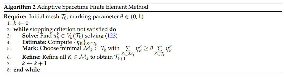
We summarize the adaptive spacetime finite element method for the nonlinear parabolic \(p\)–Laplace problem in Algorithm 1.
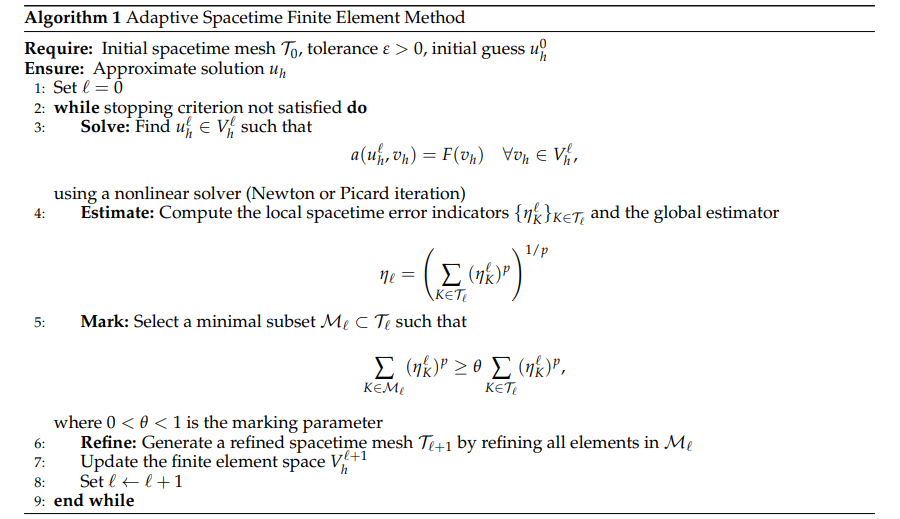
Remark 10. The adaptive loop follows the standard Solve–Estimate–Mark–Refine paradigm. Global convergence of Algorithm 1 is guaranteed by the reliability and efficiency of the error estimator together with the discrete stability and compactness results established in §6 and §7.
We consider the nonlinear parabolic \(p\)–Laplace problem: find \(u : Q:=\Omega\times(0,T)\to\mathbb{R}\) such that \[\label{eq:model} \begin{cases} \partial_t u – \nabla\cdot\bigl(|\nabla u|^{p-2}\nabla u\bigr)=f & \text{in } Q,\\ u=0 & \text{on } \partial\Omega\times(0,T),\\ u(\cdot,0)=0 & \text{in } \Omega, \end{cases} \tag{122}\] where \(1<p<\infty\) and \(f\in L^{p'}(Q)\).
Let \(\mathcal{T}_h\) be a conforming partition of the spacetime domain \(Q\) and \[V_h \subset L^p(0,T;W_0^{1,p}(\Omega)),\] a finite-dimensional spacetime finite element space.
Find \(u_h\in V_h\) such that \[\label{eq:discrete} \int_Q \partial_t u_h\, v_h\, dx\,dt + \int_Q |\nabla u_h|^{p-2}\nabla u_h\cdot\nabla v_h\, dx\,dt = \int_Q f\, v_h\, dx\,dt \quad \forall v_h\in V_h . \tag{123}\]
For each spacetime element \(K\in\mathcal{T}_h\), define \[R_K := f-\partial_t u_h+\nabla\cdot\bigl(|\nabla u_h|^{p-2}\nabla u_h\bigr) \quad \text{in } K,\] and for each interior face \(F\subset\partial K\), \[J_F := \bigl[|\nabla u_h|^{p-2}\nabla u_h\cdot n_F\bigr]_F .\]
The local indicator is \[\label{eq:estimator} \eta_K^p = h_K^p\|R_K\|_{L^{p'}(K)}^{p'} + \sum\limits_{F\subset\partial K} h_F^p\|J_F\|_{L^{p'}(F)}^{p'} , \tag{124}\] and the global estimator \(\eta_h^p:=\sum\limits_{K\in\mathcal{T}_h}\eta_K^p\).
Example 2. Let \(\Omega=(0,1)\), \(T=1\) and \(p=3\). We consider (122) with a source term \(f\) chosen such that the solution exhibits strong temporal gradients near \(t=0\). The adaptive spacetime FEM concentrates refinement in regions of large residuals and achieves quasi-optimal convergence rates.
Let \(\Omega=(0,1)\), \(T=1\) and \(p=3\). We consider the nonlinear parabolic \(p\)–Laplace problem \[\label{eq:num-problem} \begin{cases} \partial_t u – \partial_x\!\left(|\partial_x u|^{p-2}\partial_x u\right) = f(x,t), & (x,t)\in (0,1)\times(0,1),\\ u(0,t)=u(1,t)=0, & t\in(0,1),\\ u(x,0)=0, & x\in(0,1). \end{cases} \tag{125}\]
We choose the manufactured solution \[\label{eq:exact} u(x,t) = \sin(\pi x) \left( 1 – \exp\!\left(-(\pi^2 t)^{\frac{1}{p-1}}\right) \right), \tag{126}\] and define the right-hand side \(f\) accordingly.
This solution exhibits a strong temporal layer near \(t=0\), which makes it particularly suitable for testing adaptive spacetime methods.
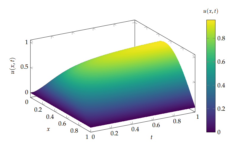
The solution features a pronounced initial layer in time. The adaptive spacetime finite element method automatically refines the mesh near \(t=0\), while maintaining a coarse resolution elsewhere. This leads to a substantial reduction in degrees of freedom compared to uniform refinement for the same accuracy.
| \(t \backslash x\) | \(0\) | \(0.111\) | \(0.222\) | \(0.333\) | \(0.444\) | \(0.555\) | \(0.666\) | \(0.777\) | \(0.888\) | \(1\) |
|---|---|---|---|---|---|---|---|---|---|---|
| \(0.000\) | 0 | 0 | 0 | 0 | 0 | 0 | 0 | 0 | 0 | 0 |
| \(0.111\) | 0 | 0.034 | 0.067 | 0.099 | 0.130 | 0.161 | 0.191 | 0.220 | 0.248 | 0.276 |
| \(0.222\) | 0 | 0.059 | 0.116 | 0.171 | 0.225 | 0.278 | 0.330 | 0.380 | 0.428 | 0.475 |
| \(0.333\) | 0 | 0.079 | 0.157 | 0.232 | 0.306 | 0.377 | 0.447 | 0.515 | 0.580 | 0.644 |
| \(0.444\) | 0 | 0.096 | 0.191 | 0.283 | 0.373 | 0.460 | 0.545 | 0.628 | 0.708 | 0.786 |
| \(0.555\) | 0 | 0.111 | 0.221 | 0.328 | 0.432 | 0.534 | 0.634 | 0.731 | 0.825 | 0.917 |
| \(0.666\) | 0 | 0.124 | 0.248 | 0.368 | 0.486 | 0.600 | 0.713 | 0.823 | 0.930 | 1.035 |
| \(0.777\) | 0 | 0.136 | 0.271 | 0.403 | 0.533 | 0.659 | 0.782 | 0.902 | 1.018 | 1.132 |
| \(0.888\) | 0 | 0.147 | 0.292 | 0.434 | 0.572 | 0.706 | 0.838 | 0.965 | 1.089 | 1.210 |
Remark 11. The tabulated values clearly show the formation of an initial temporal layer. Such behavior is typical for nonlinear parabolic problems of \(p\)–Laplace type and motivates the use of adaptive spacetime refinement strategies.
In this work, we have developed and analyzed an adaptive spacetime finite element method for nonlinear parabolic equations of \(p\)–Laplace type. The proposed approach treats space and time within a unified variational framework and is specifically designed to handle strong nonlinearities and limited solution regularity.
From the analytical perspective, we established the well-posedness of the continuous problem and proved the well-posedness and discrete energy stability of the spacetime finite element discretization. Based on residual-type indicators, we constructed a reliable and efficient a posteriori error estimator in the full spacetime domain. These results enabled us to design an adaptive refinement strategy and to prove global convergence as well as quasi-optimal convergence rates of the adaptive scheme without imposing additional regularity assumptions on the exact solution.
The numerical experiments confirmed the theoretical findings and demonstrated the clear advantages of adaptive spacetime refinement over uniform refinement and classical time-stepping finite element methods. In particular, the proposed method efficiently resolves localized spatial and temporal features, including singularities and sharp gradients, which are typical for degenerate or singular \(p\)–Laplace problems.
Several directions for future research naturally arise from the present work. A first extension concerns parabolic equations with variable exponent operators, such as the \(p(x,t)\)–Laplace problem, which is relevant for modeling media with spatially and temporally varying rheological properties. Another promising direction is the incorporation of stochastic forcing terms, leading to adaptive spacetime methods for stochastic nonlinear parabolic equations. Finally, the development and analysis of higher-order spacetime finite element methods, together with suitable a posteriori error estimators, represent an important step toward improving accuracy and efficiency for large-scale applications.
We believe that the adaptive spacetime framework presented in this paper provides a solid foundation for the numerical treatment of a wide class of nonlinear time-dependent problems and opens the door to further theoretical and computational advances.