Distance-based Indices Computation of Symmetry Molecular Structures

1. Introduction

In early years, many chemical experiments showed the evidence that the biochemical properties of chemical compounds, materials and drugs are closely related to their molecular structures. As a result, topological indices are introduced as numerical parameters of molecular graph, which play a vital role in understanding the properties of chemical compounds and are applied in disciplines such as chemistry, physics and medicine science.

In chemical graph theory, a molecular structure is expressed as a molecular graph \(G\) in which atoms are taken as vertices and chemical bonds are taken as edges. A topological index can be considered as a function \(f:G\rightarrow \mathcal{R}^{+}\). In the past 40 years, scholars introduced many topological indices, such as Wiener index, Zagreb index, harmonic index, sum connectivity index, etc which reflect certain structural characteristics of organic molecules. There were many works contributing to report these distance-based or degree-based indices of special molecular structures (See Farahani et al. [1], Jamil et al. [2], Gao and Farahani [3], Gao et al. [4, 5, 6] and Gao and Wang [7, 8, 9] for details). The notation and terminology that were used but were undefined in this paper can be found in [10].

One of oldest indices, the Wiener index was defined as the sum of distance for all pair of vertices, $$W(G)=\sum_{\{u,v\}\subseteq V(G)}d(u,v).$$ The modified Wiener index was introduced by Nikolić et al. [11] as the extension of the Wiener index which was defined as $$W_{\lambda}(G)=\sum_{\{u,v\}\subseteq V(G)}d^{\lambda}(u,v).$$ Several conclusions on modified Wiener index can be referred to Vukičević and Žerovnik [12], Vukičević and Gutman [13], Lim [14], Gorse and Žerovnik [15], Vukičević and Graovac [16], and Gutman et al. [17].

Moreover, the hyper-Wiener index and \(\lambda\)-modified hyper-Wiener index are defined as $$WW(G)=\sum_{\{u,v\}\subseteq V(G)}\frac{1}{2}(d(u,v)+d^{2}(u,v))$$ and $$WW_{\lambda}(G)=\sum_{\{u,v\}\subseteq V(G)}\frac{1}{2}(d^{\lambda}(u,v)+d^{2\lambda}(u,v)),$$ respectively. Some important contributions on hyper-Wiener index can be found in Gutman [18], Gutman and Furtula [19], Eliasi and Taeri [20, 21], Iranmanesh et al. [22], Yazdani and Bahrami [23], Behtoei et al. [24], Mansour and Schork [25], Heydari [26], Ashrafi et al. [27], and Heydari [28].

The Harary index was introduced independently by Plavšić et al. [29] and Ivanciuc et al. [30] in 1993, as $$H(G)=\sum_{\{u,v\}\subseteq V(G)}\frac{1}{d(u,v)}.$$ Its corresponding Harary polynomial can be defined as $$H(G,x)=\sum_{\{u,v\}\subseteq V(G)}\frac{1}{d(u,v)}x^{d(u,v)}.$$ The second and third Harary indices are defined as $$H_{1}(G)=\sum_{\{u,v\}\subseteq V(G)}\frac{1}{d(u,v)+1},$$ $$H_{2}(G)=\sum_{\{u,v\}\subseteq V(G)}\frac{1}{d(u,v)+2}.$$ More generally, the generalized Harary index was introduced by Das et al. [31] which is defined as $$H_{t}(G)=\sum_{\{u,v\}\subseteq V(G)}\frac{1}{d(u,v)+t},$$ where \(t\in\mathcal{N}\) is a non-negative integer. Hence, Harary index is a special case of generalized Harary index when \(t=0\).

One topological index related to Wiener index is the reciprocal complementary Wiener (RCW) index which is defined by Zhou et al. [32] and can be defined as $$RCW(G)=\sum_{\{u,v\}\subseteq V(G)}\frac{1}{D(G)+1-d(u,v)},$$ where \(D(G)\) is the diameter of molecular graph \(G\). In what follows, we always denote \(D(G)\) as the diameter of molecular graph \(G\).

Furthermore, the multiplicative version of the Wiener index was defined by Gutman et al. [33, 34] as $$\pi(G)=\prod_{\{u,v\}\subseteq V(G)}d(u,v).$$ The logarithm of multiplicative Wiener index was defined as $$\Pi(G)=\ln\sqrt{2\prod_{\{u,v\}\subseteq V(G)}d(u,v)}.$$

So far, many mathematical approaches are given to calculate different topological indices and received good results. Since most of the chemical compounds have symmetric structures. It inspires us to consider the computation of topological indices by using group theory. We use the automorphism groups and its orbits to simplify the computation of molecular graphs for some distance-based indices.

2. Main results and proofs

To discuss the symmetry molecular structures, we should first introduce symmetry operations which are defined as operations that move a fixed molecule structure from a previous condition to another, and any two states can't be differentiated from each other. Obviously, all the symmetry operations on a molecular structure constitute a group which is called the point group of the molecular structure.

When an element \(p\) of point group \(P\) (i.e., a symmetry operation on the molecular structure) operates on the molecular graph, it provides the vertices of the molecular graph a permutation. We denote \(p(v)\) as the image of vertex \(v\) under the operation \(p\). If there exists a \(p\in P\) that satisfies \(p(v)=u\) for two vertices \(v\) and \(u\), then we define an equivalence binary relation denoted by \(v\sim u\). By means of this equivalent relation, the vertex set is divided into several equivalence classes: \(\Theta_{1},\cdots,\Theta_{r}\). Each \(\Theta_{i}\) can be called an orbit of point group \(P\), and the number of vertices of each orbit \(|\Theta_{i}|\) is called the length of the orbit \(\Theta_{i}\). By the knowledge of group theory, we know that if \(v\in \Theta_{i}\) then \(|\Theta_{i}|=\frac{|P|}{|P_{v}|}\), where \(P_{v}=\{p|p\in P,p(v)=v\}\). The group called transitive if it has only one orbit, and it is called intransitive otherwise. Moreover, we can define the orbits of subgroup \(H\) in similar way which could also be either transitive or intransitive.

Set

1. \(W_{\lambda}(v,G)=\sum_{u\in V(G)}d^{\lambda}(u,v),\)
2. \(WW(v,G)=\frac{1}{2}\sum_{u\in V(G)}(d(u,v)+d^{2}(u,v)),\)
3. \(WW_{\lambda}(v,G)=\frac{1}{2}\sum_{u\in V(G)}(d^{\lambda}(u,v)+d^{2\lambda}(u,v)),\)
4. \(H(v,G)=\sum_{u\in V(G)}\frac{1}{d(u,v)},\)
5. \(H(v,G,x)=\sum_{u\in V(G)}\frac{1}{d(u,v)}x^{d(u,v)},\)
6. \(H_{1}(v,G)=\sum_{u\in V(G)}\frac{1}{d(u,v)+1},\)
7. \(H_{2}(v,G)=\sum_{u\in V(G)}\frac{1}{d(u,v)+2},\)
8. \(H_{t}(v,G)=\sum_{u\in V(G)}\frac{1}{d(u,v)+t},\)
9. \(RCW(v,G)=\sum_{u\in V(G)}\frac{1}{D(G)+1-d(u,v)},\)
10. \(\pi(v,G)=\prod_{u\in V(G)}d(u,v).\)

Hence, we have

1. \(W_{\lambda}(G)=\frac{1}{2}\sum_{v\in V(G)}W_{\lambda}(v,G) \;\; \;\;\;\;\;\;\;\;\;\; \;\; \;\;\;\;\;\;\;\;\;\; \;\; \;\;\;\;\;\;\;\;\;\; \;\; \;\;\;\;\;\;\;\;\;\; \;\; \;\;\;\;\;\;\;\;\;\; \;\; \;\;\;\;\;\;\;\;\;\; (1)\)
2. \(WW(G)=\frac{1}{2}\sum_{v\in V(G)}WW(v,G),\)
3. \(WW_{\lambda}(G)=\frac{1}{2}\sum_{v\in V(G)}WW_{\lambda}(v,G),\)
4. \(H(G)=\frac{1}{2}\sum_{v\in V(G)}H(v,G),\)
5. \(H(G,x)=\frac{1}{2}\sum_{v\in V(G)}H(v,G,x),\)
6. \(H_{1}(G)=\frac{1}{2}\sum_{v\in V(G)}H_{1}(v,G),\)
7. \(H_{2}(G)=\frac{1}{2}\sum_{v\in V(G)}H_{2}(v,G),\)
8. \(H_{t}(G)=\frac{1}{2}\sum_{v\in V(G)}H_{t}(v,G),\)
9. \(RCW(G)=\frac{1}{2}\sum_{v\in V(G)}RCW(v,G),\)
10. \(\pi(G)=\sqrt{\prod_{v\in V(G)}\pi(v,G)},\)
11. \(\Pi(G)=\ln\sqrt{2\sqrt{\prod_{v\in V(G)}\pi(v,G)}}.\)

Following theorem is about the calculation of different topological indices when the point group is not necessarily transitive.

Theroem 2.1. Let \(H\unlhd P_{G}\) be a subgroup of \(P_{G}\), and \(\Theta_{1}, \Theta_{2},\cdots, \Theta_{r}\) are the orbits of \(H\) and \(u_{i}\in\Theta_{i}\), \(i=1,2,\cdots,r\). Then, we have

1. \(W_{\lambda}(G)=\sum_{i=1}^{r}\sum_{j=i+1}^{r}|\Theta_{i}|\sum_{u\in\Theta_{j}}d^{\lambda}(u,u_{i})+\frac{1}{2}\sum_{i=1}^{r}|\Theta_{i}|\sum_{v\in \Theta_{i}}d^{\lambda}(v,\\u_{i}),\)
2. \(WW(G)=\frac{1}{2}\sum_{i=1}^{r}\sum_{j=i+1}^{r}|\Theta_{i}|\sum_{u\in\Theta_{j}}(d(u,u_{i})+d^{2}(u,u_{i}))+\frac{1}{2}\sum_{i=1}^{r}|\Theta_{i}|\\\sum_{v\in \Theta_{i}}(d(v,u_{i})+d^{2}(v,u_{i})),\)
3. \(WW_{\lambda}(G)=\frac{1}{2}\sum_{i=1}^{r}\sum_{j=i+1}^{r}|\Theta_{i}|\sum_{u\in\Theta_{j}}(d^{\lambda}(u,u_{i})+d^{2\lambda}(u,u_{i}))+\frac{1}{2}\sum_{i=1}^{r}\\| \Theta_{i}|\sum_{v\in \Theta_{i}}(d^{\lambda}(v,u_{i})+d^{2\lambda}(v,u_{i})),\)
4. \(H(G)=\sum_{i=1}^{r}\sum_{j=i+1}^{r}|\Theta_{i}|\sum_{u\in\Theta_{j}}\frac{1}{d(u,u_{i})}+\frac{1}{2}\sum_{i=1}^{r}|\Theta_{i}|\sum_{v\in \Theta_{i}}\frac{1}{d(v,u_{i})},\)
5. \(H(G,x)=\sum_{i=1}^{r}\sum_{j=i+1}^{r}|\Theta_{i}|\sum_{u\in\Theta_{j}}\frac{1}{d(u,u_{i})}x^{d(u,u_{i})}+\frac{1}{2}\sum_{i=1}^{r}|\Theta_{i}|\sum_{v\in \Theta_{i}}\\ \frac{1}{d(v,u_{i})}x^{d(v,u_{i})},\)
6. \(H_{t}(G)=\sum_{i=1}^{r}\sum_{j=i+1}^{r}|\Theta_{i}|\sum_{u\in\Theta_{j}}\frac{1}{d(u,u_{i})+t}+\frac{1}{2}\sum_{i=1}^{r}|\Theta_{i}|\sum_{v\in \Theta_{i}}\frac{1}{d(v,u_{i})+t},\)
7. \(RCW(G)=\sum_{i=1}^{r}\sum_{j=i+1}^{r}|\Theta_{i}|\sum_{u\in\Theta_{j}}\frac{1}{D(G)+1-d(u,u_{i})}+\frac{1}{2}\sum_{i=1}^{r}|\Theta_{i}|\sum_{v\in \Theta_{i}}\\ \frac{1}{D(G)+1-d(v,u_{i})},\)
8. \(\pi(G)=\prod_{i=1}^{r}\prod_{j=i+1}^{r}\prod_{u\in\Theta_{j}}d^{|\Theta_{i}|}(u,u_{i})\times\sqrt{\prod_{i=1}^{r}\prod_{v\in \Theta_{i}}d^{|\Theta_{i}|}(v,u_{i})},\)
9. \(\Pi(G)=\ln\sqrt{2\prod_{i=1}^{r}\prod_{j=i+1}^{r}\prod_{u\in\Theta_{j}}d^{|\Theta_{i}|}(u,u_{i})\times\sqrt{\prod_{i=1}^{r}\prod_{v\in \Theta_{i}}d^{|\Theta_{i}|}(v,u_{i})}}.\)

Proof. We only prove for \(W_{\lambda}(G)\). The remaining cases can be proved in similar fashion. Since \(W_{\lambda}(u,G)\) is equal to the sum of all vertices in the same orbit, we infer \begin{eqnarray*} \sum_{w\in V(G)}W_{\lambda}(w,G)&=&\sum_{i=1}^{r}\sum_{w\in \Theta_{i}}W_{\lambda}(w,G)\\&=&\sum_{i=1}^{r}|\Theta_{i}|W_{\lambda}(u_{i},G)\\ &=&\sum_{i=1}^{r}|\Theta_{i}|\sum_{j=1}^{r}\sum_{y\in \Theta_{i}}d^{\lambda}(u_{i},y)\\&=&\sum_{i=1}^{r}\sum_{j=1}^{r}|\Theta_{i}|\sum_{y\in \Theta_{i}}d^{\lambda}(u_{i},y)\\ &=&2\sum_{i=1}^{r}\sum_{j=i+1}^{r}|\Theta_{i}|\sum_{y\in\Theta_{i}}d^{\lambda}(y,u_{i})+\sum_{i=1}^{r}|\Theta_{i}|\sum_{z\in \Theta_{i}}d^{\lambda}(z,u_{i}). \end{eqnarray*} Hence, in terms of (1), \begin{eqnarray*}W_{\lambda}(G)&=&\frac{1}{2}\sum_{w\in V(G)}W_{\lambda}(w,G)\\ &=&\sum_{i=1}^{r}\sum_{j=i+1}^{r}|\Theta_{i}|\sum_{u\in\Theta_{j}}d^{\lambda}(u,u_{i})+\frac{1}{2}\sum_{i=1}^{r}|\Theta_{i}|\sum_{v\in \Theta_{i}}d^{\lambda}(v,u_{i}). \end{eqnarray*} Hence, the desired result is obtained.

The next result is about the computation of topological indices when the point group of the molecular graph is transitive.

Lemma 2.2. If the point group \(P_{G}\) of the molecular graph is transitive. Then for any \(v\in V(G)\), we have

1. \(W_{\lambda}(G)=\frac{|V(G)|}{2}W_{\lambda}(v,G),\)
2. \(WW(G)=\frac{|V(G)|}{4}WW(v,G),\)
3. \(WW_{\lambda}(G)=\frac{|V(G)|}{4}WW_{\lambda}(v,G),\)
4. \(H(G)=\frac{|V(G)|}{2}H(v,G),\)
5. \(H(G,x)=\frac{|V(G)|}{2}H(v,G,x),\)
6. \(H_{t}(G)=\frac{|V(G)|}{2}H_{t}(v,G),\)
7. \(RCW(G)=\frac{|V(G)|}{2}RCW(v,G),\)
8. \(\pi(G)=\sqrt{\pi^{|V(G)|}(v,G)},\)
9. \(\Pi(G)=\ln\sqrt{2\sqrt{\pi^{|V(G)|}(v,G)}}.\)

In terms of Lemma 2.2, to calculate the distance-based topological indices of the molecular graph with transitive point group, we only need to choose any vertex \(v\in V(G)\) and calculate the distances between \(v\) and \(u\in V(G)-\{v\}\). Take a subgroup \(H\) of \(P_{G}\), which is not necessarily transitive even if \(P_{G}\) is transitive. Now, the vertex set \(V(G)\) can be divided into orbits of \(H\) such that \(\Theta_{1},\Theta_{2},\cdots,\Theta_{r}\) with \((|\Theta_{1}|\le|\Theta_{2}|\le\cdots|\Theta_{r}|\).

Theorem 2.3. Let \(v_{i}\in \Theta_{i}\), \(i=1,2,\cdots,r\). Then,

1. \(W_{\lambda}(v_{1},G)=\frac{1}{|\Theta_{1}|}\sum_{u\in \Theta_{1}}\sum_{i=1}^{r}|\Theta_{i}|d^{\lambda}(u,v_{i}),\)
2. \(WW(v_{1},G)=\frac{1}{|\Theta_{1}|}\sum_{u\in \Theta_{1}}\sum_{i=1}^{r}\frac{|\Theta_{i}|}{2}(d(u,v_{i})+d^{2}(u,v_{i})),\)
3. \(WW_{\lambda}(v_{1},G)=\frac{1}{|\Theta_{1}|}\sum_{u\in \Theta_{1}}\sum_{i=1}^{r}\frac{|\Theta_{i}|}{2}(d^{\lambda}(u,v_{i})+d^{2\lambda}(u,v_{i})),\)
4. \(H(v_{1},G)=\frac{1}{|\Theta_{1}|}\sum_{u\in \Theta_{1}}\sum_{i=1}^{r}\frac{|\Theta_{i}|}{d(u,v_{i})},\)
5. \(H(v_{1},G,x)=\frac{1}{|\Theta_{1}|}\sum_{u\in \Theta_{1}}\sum_{i=1}^{r}\frac{|\Theta_{i}|}{d(u,v_{i})}x^{d(u,v_{i})},\)
6. \(H_{t}(v_{1},G)=\frac{1}{|\Theta_{1}|}\sum_{u\in \Theta_{1}}\sum_{i=1}^{r}\frac{|\Theta_{i}|}{d(u,v_{i})+t},\)
7. \(RCW(v_{1},G)=\frac{1}{|\Theta_{1}|}\sum_{u\in \Theta_{1}}\sum_{i=1}^{r}\frac{|\Theta_{i}|}{D(G)+1-d(u,v_{i})}.\)

Proof. Since \(P_{G}\) is transitive, we get \begin{eqnarray*} W_{\lambda}(v_{1},G)&=&\frac{1}{|\Theta_{1}|}\sum_{u\in \Theta_{1}}\sum_{z\in V(G)}d^{\lambda}(u,z)\\ &=&\frac{1}{|\Theta_{1}|}\sum_{u\in \Theta_{1}}\sum_{i=1}^{r}\sum_{z\in \Theta_{i}}d^{\lambda}(u,z)\\ &=&\frac{1}{|\Theta_{1}|}\sum_{i=1}^{r}\sum_{z\in \Theta_{i}}\sum_{u\in \Theta_{1}}d^{\lambda}(u,z). \end{eqnarray*} For any \(i\) and any \(z\in \Theta_{i}\), there exist \(h_{i}\in H\) satisfying \(h_{i}(z)=v_{i}\). Therefore, \begin{eqnarray*} \sum_{z\in \Theta_{i}}\sum_{u\in \Theta_{1}}d^{\lambda}(u,z)&=&\sum_{z\in \Theta_{i}}\sum_{u\in \Theta_{1}}d^{\lambda}(h_{i}(u),h_{i}(z))\\ &=&\sum_{z\in \Theta_{i}}\sum_{h_{i}(u)\in \Theta_{1}}d^{\lambda}(h_{i}(u),v_{i})\\&=&|\Theta_{i}|\sum_{h_{i}(u)\in \Theta_{1}}d^{\lambda}(h_{i}(u),v_{i})\\ &=&|\Theta_{i}|\sum_{v\in\Theta_{1}}d^{\lambda}(v,v_{i}). \end{eqnarray*} Consequently, we yield \begin{eqnarray*} W_{\lambda}(v_{1},G)&=&\frac{1}{|\Theta_{1}|}\sum_{i=1}^{r}\sum_{u\in \Theta_{1}}\sum_{z\in \Theta_{i}}d^{\lambda}(u,z)\\ &=&\frac{1}{|\Theta_{1}|}\sum_{i=1}^{r}|\Theta_{i}|\sum_{v\in\Theta_{1}}d^{\lambda}(v,v_{i})\\ &=&\frac{1}{|\Theta_{1}|}\sum_{v\in\Theta_{1}}\sum_{i=1}^{r}|\Theta_{i}|d^{\lambda}(v,v_{i}). \end{eqnarray*} The remaining parts follows similarly, hence, we complete the proof.

In theorem 2.3, we can see that for a vertex \(v_{1}\in\Theta_{1}\), we do not need to compute all distances between \(v_{1}\) and \(V(G)-\{v_{1}\}\). It is enough to select one vertex from \(\Theta_{i}\). In real practice, we select a subgroup \(H\) so that \(\Theta_{1}\) is as small as possible in order to simplify the calculation. Specially, if \(|\Theta_{1}|=1\) (\(H\) fixes \(v_{1}\)), we only count \(r-1\) times. Hence, we can give the following corollary.

Corollary 2.4. Let \(v_{i}\in\Theta_{i}\), \(i=1,2,\cdots,r\). Assume that \(|\Theta_{1}|=1\). We get

1. \(W_{\lambda}(v_{1},G)=\sum_{i=2}^{r}|\Theta_{i}|d^{\lambda}(v_{1},v_{i}),\)
2. \(WW(v_{1},G)=\sum_{i=2}^{r}|\Theta_{i}|\frac{d(v_{1},v_{i})+d^{2}(v_{1},v_{i})}{2},\)
3. \(WW_{\lambda}(v_{1},G)=\sum_{i=2}^{r}|\Theta_{i}|\frac{d^{\lambda}(v_{1},v_{i})+d^{2\lambda}(v_{1},v_{i})}{2},\)
4. \(H(v_{1},G)=\sum_{i=2}^{r}|\Theta_{i}|\frac{1}{d(v_{1},v_{i})},\)
5. \(H(v_{1},G,x)=\sum_{i=2}^{r}|\Theta_{i}|\frac{1}{d(v_{1},v_{i})}x^{d(v_{1},v_{i})},\)
6. \(H_{t}(v_{1},G)=\sum_{i=2}^{r}|\Theta_{i}|\frac{1}{d(v_{1},v_{i})+t},\)
7. \(RCW(v_{1},G)=\sum_{i=2}^{r}|\Theta_{i}|\frac{1}{D(G)+1-d(v_{1},v_{i})},\)
8. \(\pi(v_{1},G)=\prod_{i=2}^{r}d^{|\Theta_{i}|}(v_{1},v_{i}),\)
9. \(\Pi(v_{1},G)=\ln\sqrt{2\prod_{i=2}^{r}d^{|\Theta_{i}|}(v_{1},v_{i})}.\)

In order to reduce the computation steps of the distance-based topological indices, note that a large number of the molecular structures have the layered structure such that the different orbits have consecutive distances from a fixed vertex. In such a situation, we have following theorem.

Theorem 2.5. Assume that \(P_{G}\) is transitive and \(H\unlhd P_{G}\) is a subgroup with orbits \(\Theta_{1},\Theta_{2},\cdots,\Theta_{r}\) such that \(|\Theta_{i}|=1\). Let \(v_{i}\in\Theta_{i}\) for \(i=1,2,\cdots,r\). Then we have

1. \(W_{\lambda}(G)=\frac{n}{2}\sum_{j=2}^{r}|\Theta_{k_{j}}|(j-1)^{\lambda},\)
2. \(WW(G)=\frac{n}{2}\sum_{j=2}^{r}|\Theta_{k_{j}}|\frac{j^{2}-j}{2},\)
3. \(WW_{\lambda}(G)=\frac{n}{2}\sum_{j=2}^{r}|\Theta_{k_{j}}|\frac{(j-1)^{\lambda}+(j-1)^{2\lambda}}{2},\)
4. \(H(G)=\frac{n}{2}\sum_{j=2}^{r}|\Theta_{k_{j}}|\frac{1}{j-1},\)
5. \(H(G,x)=\frac{n}{2}\sum_{j=2}^{r}|\Theta_{k_{j}}|\frac{1}{j-1}x^{j-1},\)
6. \(H_{t}(G)=\frac{n}{2}\sum_{j=2}^{r}|\Theta_{k_{j}}|\frac{1}{j+t-1},\)
7. \(RCW(G)=\frac{n}{2}\sum_{j=2}^{r}|\Theta_{k_{j}}|\frac{1}{D(G)+2-j},\)
8. \(\pi(G)=(\prod_{j=2}^{r}(j-1)^{|\Theta_{k_{j}}|})^{\frac{n}{2}},\)
9. \(\Pi(G)=\ln\sqrt{(\prod_{j=2}^{r}(j-1)^{|\Theta_{k_{j}}|})^{\frac{n}{2}}}.\)

Proof. Science the molecular graphs are connected and all the elements in the same orbit have equal distances from \(v_{1}\), the orbits saturate the vacancy between \(\Theta_{1}\) and \(\Theta_{k}\) by means of their distances from \(v_{1}\). Since only \(r-1\) orbits different from \(\Theta_{1}\) and \(d(v_{1},v_{k})\ge r-1\), we infer that the orbits run consecutively between \(\Theta_{1}\) and \(\Theta_{k}\), which reveals that the vertices \(v_{1},v_{2},\cdots,v_{r}\) can be permuted into \(v_{k_{1}},v_{k_{2}},\cdots,v_{k_{r}}\) with \(k_{1}=1\) and \(k_{r}=k\) satisfies \(d(v_{1},v_{k_{j}})=j-1\), \(j=1,2,\cdots,r\). Therefore, \begin{eqnarray*} W_{\lambda}(G)&=&\frac{n}{2}W_{\lambda}(v_{1},G)\\&=&\frac{n}{2}\sum_{i=2}^{r}|\Theta_{i}|d^{\lambda}(v_{1},v_{i})\\ &=&\frac{n}{2}\sum_{j=2}^{r}|\Theta_{k_{j}}|d^{\lambda}(v_{1},v_{k_{j}})\\&=&\frac{n}{2}\sum_{j=2}^{r}|\Theta_{k_{j}}|(j-1)^{\lambda}. \end{eqnarray*} The remaining cases can be easily proved in similar fashion.

For the presentation of examples in the next section, we should mention that all the regular polyhedrons meet the conditions in the Theorem 2.5.

3. Computation Examples

In this section, we give five illustrative examples to explain our method. In the following contexts, we always assume that $n$ is the number of vertex in molecular graph $G$ and the regular polyhedrons meet the conditions of the theorem 2.5.

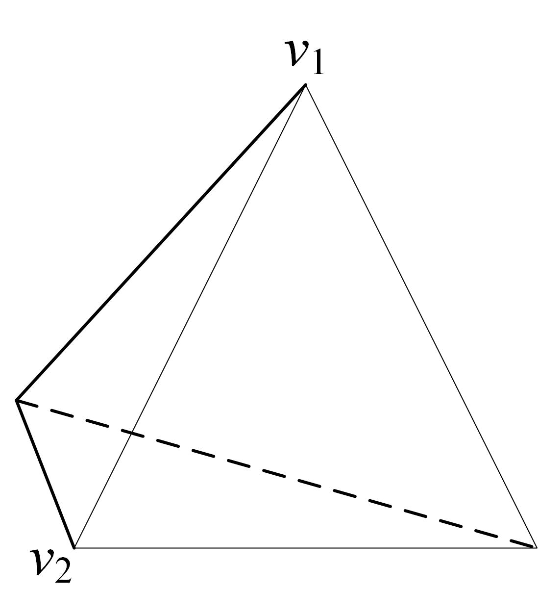
Example 3.1. [Computation on tetrahedron] The structure of tetrahedron (denoted by \(G_{1}\)) can refer to Figure 1. Let \(P_{G_{1}}\) be its point group. We need first determine the subgroup \(R\unlhd P_{G_{1}}\) of all the rotation in \(P_{G_{1}}\). The elements consisting of \(R\) are as follows: (1) the identity; (2) rotations through the angle \(\pi\) about each of three axes joining the midpoints of opposite edges; (3) rotations through angles of \(\frac{2\pi}{3}\) and \(\frac{4\pi}{3}\) on the each of four axes joining vertices with centers of opposite faces. So, we have \(|R|=12\).

Clearly, \(R\) and \(P_{G_{1}}\) are transitive. Select \(H\) as the identity plus the set of all rotations around the axis joining \(v_{1}\) with the center of the opposite face through angles of \(\frac{2\pi}{3}\) and \(\frac{4\pi}{3}\) anticlockwise. We yield two orbits with representatives \(v_{1}\), \(v_{2}\) as presented in the Figure 1. Applying \(|\Theta_{i}|=\frac{|P|}{|P_{v}|}\), we infer \(|\Theta_{1}|=1\), \(|\Theta_{2}|=3\). According to theorem 2.5, we get

1. \(W_{\lambda}(G_{1})=\frac{n}{2}\sum_{j=2}^{r}|\Theta_{k_{j}}|(j-1)^{\lambda}=\frac{4}{2}\cdot3=6,\)
2. \(WW(G_{1})=\frac{n}{2}\sum_{j=2}^{r}|\Theta_{k_{j}}|\frac{j^{2}-j}{2}=\frac{4}{2}\cdot3\cdot\frac{1}{2}(1+1^{2})=6,\)
3. \(WW_{\lambda}(G_{1})=\frac{n}{2}\sum_{j=2}^{r}|\Theta_{k_{j}}|\frac{(j-1)^{\lambda}+(j-1)^{2\lambda}}{2}=\frac{4}{2}\cdot3\cdot\frac{1}{2}(1^{\lambda}+1^{2\lambda})=6,\)
4. \(H(G_{1})=\frac{n}{2}\sum_{j=2}^{r}|\Theta_{k_{j}}|\frac{1}{j-1}=\frac{4}{2}\cdot3=6,\)
5. \(H(G_{1},x)=\frac{n}{2}\sum_{j=2}^{r}|\Theta_{k_{j}}|\frac{1}{j-1}x^{j-1}=\frac{4}{2}\cdot3\cdot x=6x,\)
6. \(H_{t}(G_{1})=\frac{n}{2}\sum_{j=2}^{r}|\Theta_{k_{j}}|\frac{1}{j+t-1}=\frac{4}{2}\cdot3\cdot\frac{1}{1+t}=\frac{6}{1+t},\)
7. \(RCW(G_{1})=\frac{n}{2}\sum_{j=2}^{r}|\Theta_{k_{j}}|\frac{1}{D(G)+2-j}=\frac{4}{2}\cdot3\cdot\frac{1}{1+1-1}=6,\)
8. \(\pi(G_{1})=(\prod_{j=2}^{r}(j-1)^{|\Theta_{k_{j}}|})^{\frac{n}{2}}=1,\)
9. \(\Pi(G_{1})=\ln\sqrt{(\prod_{j=2}^{r}(j-1)^{|\Theta_{k_{j}}|})^{\frac{n}{2}}}=\ln\sqrt{2}.\)

Example 3.2. [Computation on cube] \noindent The structure of cube (denoted as \(G_{2}\)) can refer to Figure 2. In this case, the subgroup \(R\unlhd P_{G_{2}}\) of all the rotations consists of the follows: (1) rotations through the angle \(\pi\) on each of six axes joining midpoints of diagonally opposite edges; (2) rotations through angles of \(\frac{\pi}{2}\) and \(\frac{3\pi}{2}\) about each of four axes joining extreme opposite vertices; (3) rotations through angles of \(\frac{\pi}{2},\pi\), and \(\frac{3\pi}{2}\) about each of three axes joining the centers of opposite faces. Thus, by simple computation, we get \(|R|=24\).

Clearly, \(R\) and \(P_{G_{2}}\) are both transitive. \(H\) is selected as in the first instance but the rotations are around the axis joining the two opposite vertices \(v_{1}\) and \(v_{3}\). We get four orbits with representatives \(v_{1}\), \(v_{2}\), \(v_{3}\) and \(v_{4}\) as presented in the Figure 2. In view of \(|\Theta_{i}|=\frac{|P|}{|P_{v}|}\), we yield \(|\Theta_{1}|=|\Theta_{4}|=1\), \(|\Theta_{2}|=|\Theta_{3}|=3\). Applying theorem 2.5, we get

1. \(W_{\lambda}(G_{2})=\frac{n}{2}\sum_{j=2}^{r}|\Theta_{k_{j}}|(j-1)^{\lambda}=\frac{8}{2}(3+3\cdot2^{\lambda}+3^{\lambda})=12+12\cdot2^{\lambda}+4\cdot3^{\lambda},\)
2. \(WW(G_{2})=\frac{n}{2}\sum_{j=2}^{r}|\Theta_{k_{j}}|\frac{j^{2}-j}{2}=\frac{8}{2}(\frac{3}{2}(1+1)+\frac{3}{2}(2+4)+\frac{3+9}{2})=72,\)
3. \(WW_{\lambda}(G_{2})=\frac{n}{2}\sum_{j=2}^{r}|\Theta_{k_{j}}|\frac{(j-1)^{\lambda}+(j-1)^{2\lambda}}{2}=\frac{8}{2}(\frac{3}{2}(1+1) +\frac{3}{2}(2^{\lambda}+4^{\lambda})+\frac{3^{\lambda}+9^{\lambda}}{2}) =12+6(2^{\lambda}+4^{\lambda})+2(3^{\lambda}+9^{\lambda}),\)
4. \(H(G_{2})=\frac{n}{2}\sum_{j=2}^{r}|\Theta_{k_{j}}|\frac{1}{j-1}=\frac{8}{2}(3+\frac{3}{2}+\frac{1}{3})=\frac{58}{3},\)
5. \(H(G_{2},x)=\frac{n}{2}\sum_{j=2}^{r}|\Theta_{k_{j}}|\frac{1}{j-1}x^{j-1}=\frac{8}{2}(3x+\frac{3}{2}x^{2}+\frac{1}{3}x^{3})=12x+6x^{2}+\frac{4}{3}x^{3},\)
6. \(H_{t}(G_{2})=\frac{n}{2}\sum_{j=2}^{r}|\Theta_{k_{j}}|\frac{1}{j+t-1}=4(\frac{3}{1+t}+\frac{3}{2+t}+\frac{1}{3+t}),\)
7. \(RCW(G_{2})=\frac{n}{2}\sum_{j=2}^{r}|\Theta_{k_{j}}|\frac{1}{D(G)+2-j}=\frac{8}{2}(\frac{3}{3}+\frac{3}{2}+\frac{1}{1})=14,\)
8. \(\pi(G_{2})=(\prod_{j=2}^{r}(j-1)^{|\Theta_{k_{j}}|})^{\frac{n}{2}}=(1^{3}\cdot2^{3}\cdot3)^{\frac{8}{2}}=331776,\)
9. \(\Pi(G_{2})=\ln\sqrt{(\prod_{j=2}^{r}(j-1)^{|\Theta_{k_{j}}|})^{\frac{n}{2}}}=\ln576\sqrt{2}.\)

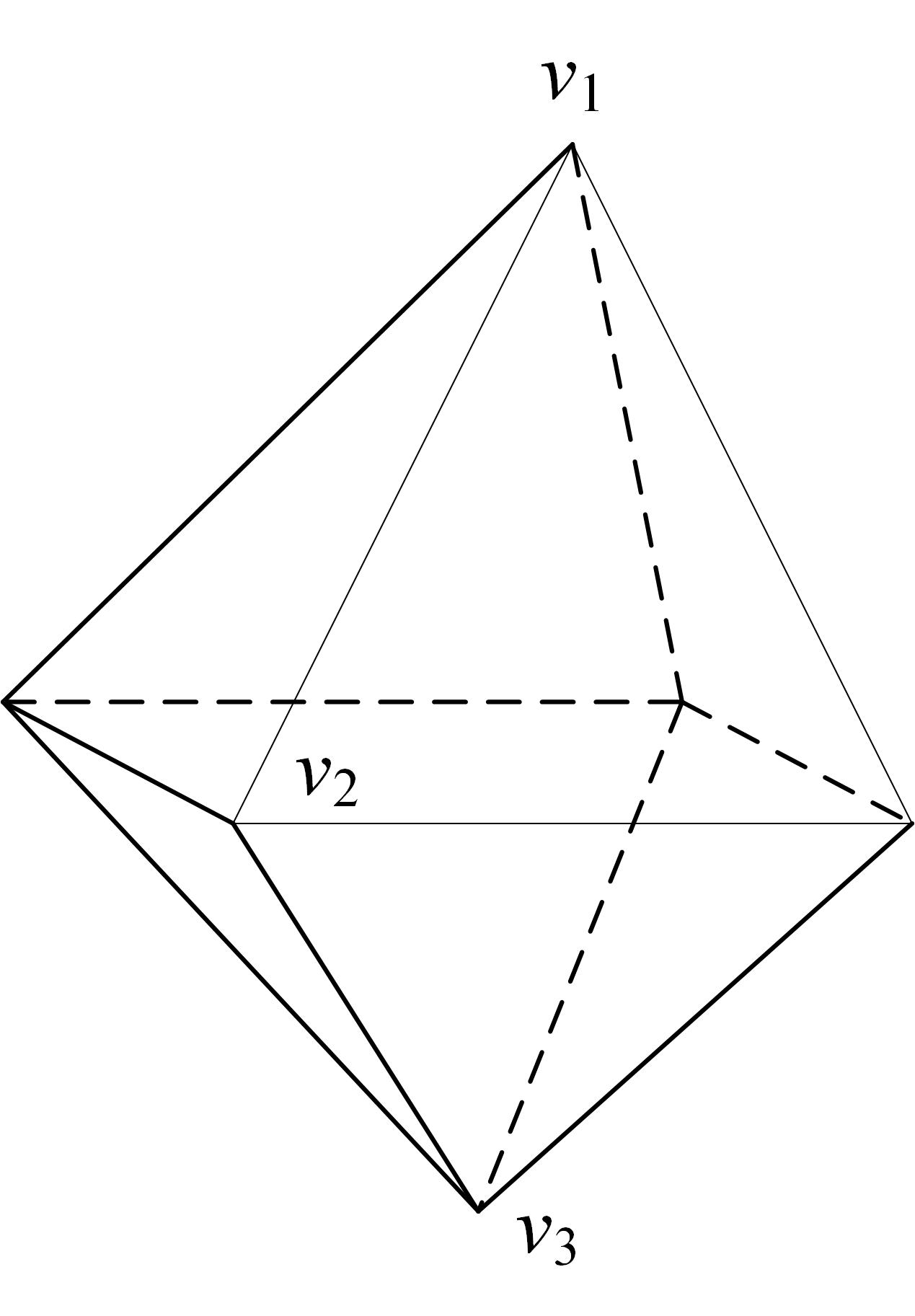
Example 3.3. [Computation on octahedron] The structure of octahedron (denoted by \(G_{3}\)) can refer to Figure 3. Obviously, we can get the octahedron by adding the midpoints of adjacent faces of the cube with edges. Form this point of view, its point group is the same as that of the cube.

Furthermore, \(P_{G_{3}}\) is transitive, and all the rotations can be selected around the axis joining \(v_{1}\) and \(v_{3}\) which keep the octahedron invariant. Three orbits are obtained with representatives \(v_{i}\), \(i=1,2,3\) as depicted in the Figure 3 and \(|\Theta_{1}|=|\Theta_{3}|=1\) and \(|\Theta_{2}|=4\). By theorem 2.5, we get

1. \(W_{\lambda}(G_{3})=12+3\cdot2^{\lambda},\)
2. \(WW(G_{3})=21,\)
3. \(WW_{\lambda}(G_{3})=12+\frac{3}{2}(2^{\lambda}+4^{\lambda}),\)
4. \(H(G_{3})=\frac{27}{2},\)
5. \(H(G_{3},x)=12x+3x^{2},\)
6. \(H_{t}(G_{3})=\frac{12}{1+t}+\frac{3}{2+t},\)
7. \(RCW(G_{3})=9,\)
8. \(\pi(G_{3})=8,\)
9. \(\Pi(G_{3})=\ln4.\)

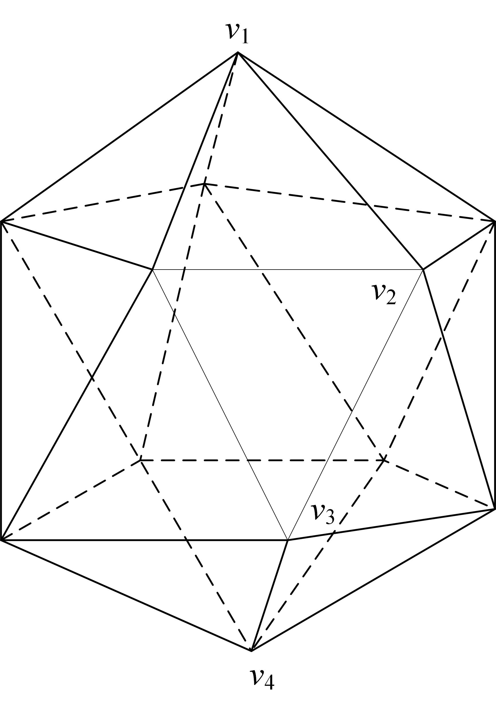
Example 3.4. [Computation on icosahedron] The structure of icosahedron (denoted by \(G_{4}\)) can refer to Figure 4. The rotation subgroup \(R\) of the point group consists: (1)the identity; (2) rotations through the angle \(\pi\) about each of fifteen axes joining midpoints of opposite edges; (3) rotations through angles of \(\frac{2\pi}{3}\) and \(\frac{4\pi}{3}\) about each of ten axes joining centers of opposite faces; (4) rotations through angles of \(\frac{2\pi}{5},\frac{4\pi}{5},\frac{6\pi}{5}\), and \(\frac{8\pi}{5}\) about each of six axes joining extreme opposite vertices. Therefore, we have \(|R|=60\).

I am raw html block.
Click edit button to change this html

Furthermore, \(R\) and \(P_{G_{4}}\) are transitive. \(H\) can be selected as the group generated by the \(\frac{2\pi}{5}\)-rotation around the axis joining \(v_{1}\) and \(v_{4}\). There are four orbits with representatives as shown in the Figure 4 and by \(|\Theta_{i}|=\frac{|P|}{|P_{v}|}\) we get \(|\Theta_{1}|=|\Theta_{4}|=1\), \(|\Theta_{2}|=|\Theta_{3}|=5\). Applying theorem 2.5, we get

1. \(W_{\lambda}(G_{4})=\frac{n}{2}\sum_{j=2}^{r}|\Theta_{k_{j}}|(j-1)^{\lambda}=\frac{12}{2}(5+5\cdot2^{\lambda}+3^{\lambda})=30+30\cdot2^{\lambda}+6\cdot3^{\lambda},\)
2. \(WW(G_{4})=\frac{n}{2}\sum_{j=2}^{r}|\Theta_{k_{j}}|\frac{j^{2}-j}{2}=\frac{12}{2}(\frac{5}{2}(1+1)+\frac{5}{2}(2+4)+\frac{3+9}{2})=156,\)
3. \(WW_{\lambda}(G_{4})=\frac{n}{2}\sum_{j=2}^{r}|\Theta_{k_{j}}|\frac{(j-1)^{\lambda}+(j-1)^{2\lambda}}{2}=\frac{12}{2} (\frac{5}{2}(1+1)+\frac{5}{2}(2^{\lambda}+4^{\lambda})+\frac{3^{\lambda}+9^{\lambda}}{2}) =30+15(2^{\lambda}+4^{\lambda})+3(3^{\lambda}+9^{\lambda}),\)
4. \(H(G_{4})=\frac{n}{2}\sum_{j=2}^{r}|\Theta_{k_{j}}|\frac{1}{j-1}=\frac{12}{2}(5+\frac{5}{2}+\frac{1}{3})=47,\)
5. \(H(G_{4},x)=\frac{n}{2}\sum_{j=2}^{r}|\Theta_{k_{j}}|\frac{1}{j-1}x^{j-1}=\frac{12}{2}(5x+\frac{5}{2}x^{2}+\frac{1}{3}x^{3})=30x+15x^{2}+2x^{3},\)
6. \(H_{t}(G_{4})=\frac{n}{2}\sum_{j=2}^{r}|\Theta_{k_{j}}|\frac{1}{j+t-1}=6(\frac{5}{1+t}+\frac{5}{2+t}+\frac{1}{3+t}),\)
7. \(RCW(G_{4})=\frac{n}{2}\sum_{j=2}^{r}|\Theta_{k_{j}}|\frac{1}{D(G)+2-j}=\frac{12}{2}(\frac{5}{3}+\frac{5}{2}+\frac{1}{1})=31,\)
8. \(\pi(G_{4})=(\prod_{j=2}^{r}(j-1)^{|\Theta_{k_{j}}|})^{\frac{n}{2}}=(1^{5}\cdot2^{5}\cdot3)^{\frac{12}{2}}=96^{6},\)
9. \(\Pi(G_{4})=\ln\sqrt{(\prod_{j=2}^{r}(j-1)^{|\Theta_{k_{j}}|})^{\frac{n}{2}}}=\ln96^{3}\sqrt{2}.\)

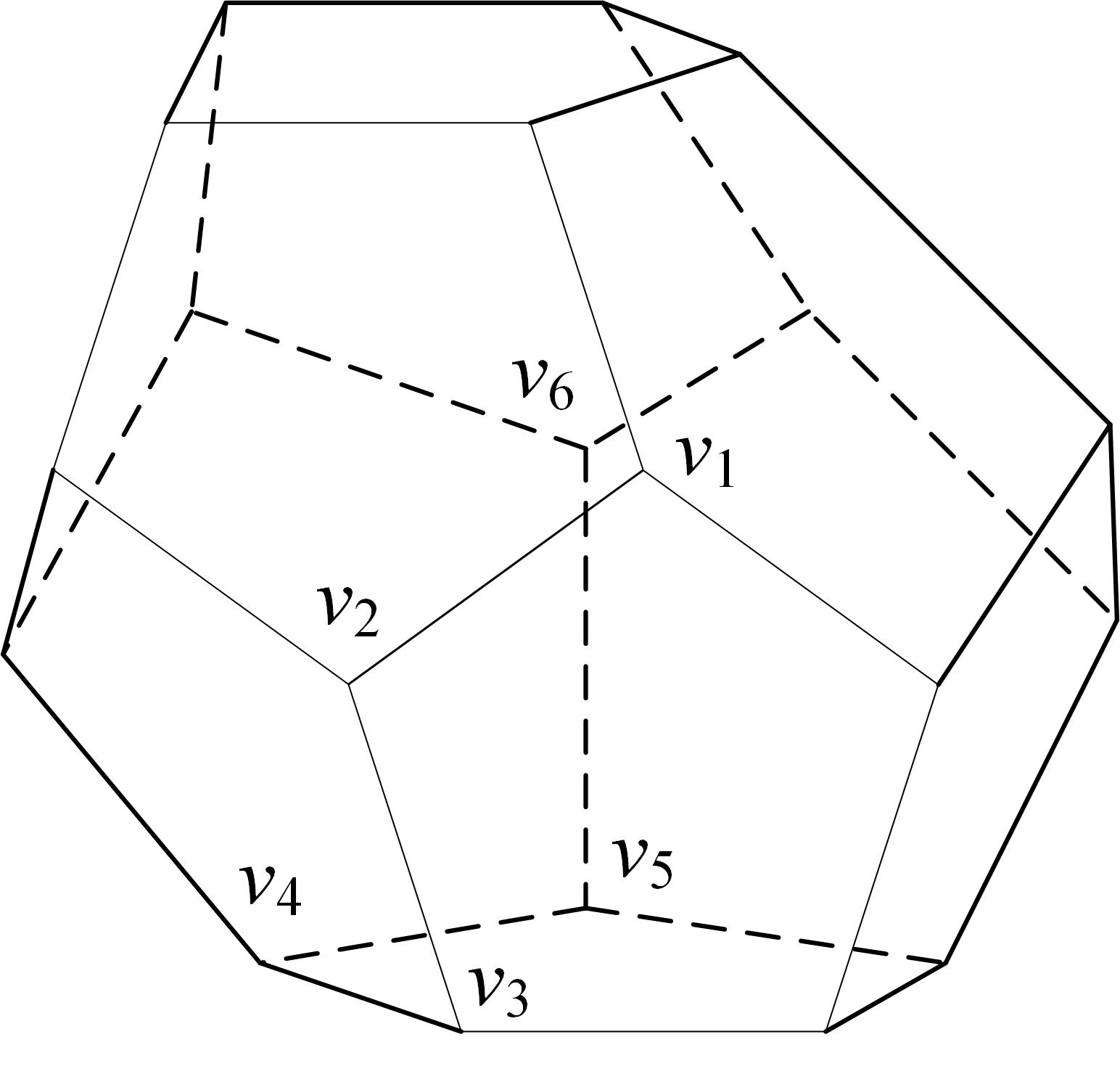
Example 3.5. [Computation on dodecahedron] The structure of dodecahedron (denoted by \(G_{5}\)) can refer to Figure 5. Similar as we discussed in the above examples, one can see that the dodecahedron and icosahedron have the same point group. Hence, \(H\) can be selected to be the group generated by the \(\frac{2\pi}{3}\)-rotation around the axis joining \(v_{1}\) and \(v_{6}\), and the reflection with respect to the plane containing \(v_{1},v_{2}\) and \(v_{6}\).

There are six orbits with representatives \(v_{i}\), \(i=1,2,\cdots,6\) as shown in the Figure 5. By simple computation, we get \(|\Theta_{1}|=|\Theta_{6}|=1\), \(|\Theta_{2}|=|\Theta_{5}|=3\) and \(|\Theta_{3}|=|\Theta_{4}|=6\). Thus, in terms of Theorem 2.5, we get

1. \( W_{\lambda}(G_{5})=\frac{n}{2}\sum_{j=2}^{r}|\Theta_{k_{j}}|(j-1)^{\lambda}=\frac{20}{2}(3+6\cdot2^{\lambda}+6\cdot3^{\lambda}+3\cdot4^{\lambda}+5^{\lambda}) =30+60\cdot2^{\lambda}+60\cdot3^{\lambda}+30\cdot4^{\lambda}+10\cdot5^{\lambda},\)
2. \( WW(G_{5})=\frac{n}{2}\sum_{j=2}^{r}|\Theta_{k_{j}}|\frac{j^{2}-j}{2} =\frac{20}{2}(\frac{3}{2}(1+1)+3(2+4)+3(3+9)+\frac{3}{2}(4+16)+\frac{1}{2}(5+25))=1020,\)
3. \( WW_{\lambda}(G_{5})=\frac{n}{2}\sum_{j=2}^{r}|\Theta_{k_{j}}|\frac{(j-1)^{\lambda}+(j-1)^{2\lambda}}{2} =\frac{20}{2}(\frac{3}{2}(1+1)+3(2^{\lambda}+4^{\lambda})+3(3^{\lambda}+9^{\lambda})+\frac{3}{2}(4^{\lambda}+16^{\lambda})+\frac{1}{2}(5^{\lambda}+25^{\lambda})) =30+30(2^{\lambda}+4^{\lambda})+30(3^{\lambda}+9^{\lambda})+15(4^{\lambda}+16^{\lambda})+5(5^{\lambda}+25^{\lambda}),\)
4. \( H(G_{5})=\frac{n}{2}\sum_{j=2}^{r}|\Theta_{k_{j}}|\frac{1}{j-1} =\frac{20}{2}(3+\frac{6}{2}+\frac{6}{3}+\frac{3}{4}+\frac{1}{5})=\frac{179}{2},\)
5. \( H(G_{5},x)=\frac{n}{2}\sum_{j=2}^{r}|\Theta_{k_{j}}|\frac{1}{j-1}x^{j-1}=\frac{20}{2}(3x+\frac{6}{2}x^{2}+\frac{6}{3}x^{3}+\frac{3}{4}x^{4}+\frac{1}{5}x^{5}) =30x+30x^{2}+20x^{3}+\frac{15}{2}x^{4}+2x^{5},\)
6. \( H_{t}(G_{5})=\frac{n}{2}\sum_{j=2}^{r}|\Theta_{k_{j}}|\frac{1}{j+t-1}=\frac{20}{2}(\frac{3}{1+t}+\frac{6}{2+t}+\frac{6}{3+t}+\frac{3}{4+t}+\frac{1}{5+t}) =\frac{30}{1+t}+\frac{60}{2+t}+\frac{60}{3+t}+\frac{30}{4+t}+\frac{10}{5+t},\)
7. \(RCW(G_{5})=\frac{n}{2}\sum_{j=2}^{r}|\Theta_{k_{j}}|\frac{1}{D(G)+2-j} =\frac{20}{2}(\frac{3}{5}+\frac{6}{4}+\frac{6}{3}+\frac{3}{2}+\frac{1}{1})=66,\)
8. \(\pi(G_{5})=(\prod_{j=2}^{r}(j-1)^{|\Theta_{k_{j}}|})^{\frac{n}{2}}=(2^{6}3^{6}4^{3}5)^{10},\)
9. \(\Pi(G_{5})=\ln\sqrt{(\prod_{j=2}^{r}(j-1)^{|\Theta_{k_{j}}|})^{\frac{n}{2}}}=\ln\sqrt{2^{61}3^{60}4^{30}5^{10}}.\)

4. Conclusion

In this paper, we mainly report the approach on how to use group theory to determine the distance-based topological indices for certain important symmetry chemical structures. Since these Wiener related and other distance-based topological indices are widely applied in the analysis of both the boiling point and melting point of chemical compounds and QSPR/QSAR study, the promising prospects of their application for the chemical, medical and pharmacy engineering will be illustrated in the theoretical conclusion that is obtained in this article.

Acknowledgments

The authors thank the reviewers for their constructive comments in improving the quality of this paper.

Competing Interests

The author(s) do not have any competing interests in the manuscript.

References

Farahani, M. R., Jamil, M. K., & Imran, M. (2016). Vertex \(PI_{v}\) topological index of titania carbon nanotubes \(TiO_{2}(m,n)\). Appl. Math. Nonl. Sci, 1(1), 175-182. [Google Scholor]
Jamil, M. K., Farahani, M. R., Imran, M., & Malik, M. A. (2016). Computing eccentric version of second zagreb index of polycyclic aromatic hydrocarbons PAHk. Appl. Math. Nonl. Sci, 1(1), 247-252.[Google Scholor]
Gao, W., & Farahani, M. R. (2016). Computing the reverse eccentric connectivity index for certain family of nanocone and fullerene structures. Journal of Nanotechnology, Volume 2016, Article ID 3129561, 6 pages. [Google Scholor]
Gao, W., Wang, W., & Farahani, M. R. (2016). Topological indices study of molecular structure in anticancer drugs. Journal of Chemistry, Volume 2016, Article ID 3216327, 8 pages.[Google Scholor]
Gao, W., Farahani, M. R., & Shi, L. (2016). Forgotten topological index of some drug structures. Acta Medica Mediterranea, 32, 579-585. [Google Scholor]
Gao, W., Shi, L., & Farahani, M. R. (2016). Distance-Based Indices for Some Families of Dendrimer Nanostars. Int. J. Appl. Math. 46(2) (2016), 168-186. [Google Scholor]
Gao, W., & Wang, W. (2014). Second atom-bond connectivity index of special chemical molecular structures. Journal of Chemistry, Volume
2014, Article ID 906254, 8 pages. [Google Scholor]
Gao, W., & Wang, W. (2015). The vertex version of weighted wiener number for bicyclic molecular structures. Computational and Mathematical Methods in Medicine, Volume 2015, Article ID 418106, 10 pages. [Google Scholor]
Gao, W., & Wang, W. (2016). The eccentric connectivity polynomial of two classes of nanotubes. Chaos, Solitons & Fractals, 89, 290-294. [Google Scholor]
Bondy, J. A., & Murty, U. S. R. (1976). Graph theory with applications (Vol. 290). London: Macmillan. [Google Scholor]
Nikolić, S., Trinajstić, N., & Randić, M. (2001). Wiener index revisited. Chemical Physics Letters, 333(3-4), 319-321. [Google Scholor]
Vukičević, D., & Žerovnik, J. (2003). New indices based on the modified Wiener indices. MATCH: communications in mathematical and in computer chemistry, 47, 119-132.[Google Scholor]
Vukičević, D., & Gutman, I. (2003). Note on a class of modified Wiener indices. MATCH: communications in mathematical and in computer chemistry, 47, 107-117.
Lim, T. C. (2004). Mass-modified Wiener indices and the boiling points for lower chloroalkanes. Acta Chim. Slov, 51(4), 611-618. [Google Scholor]
Gorse, M., & Zerovnik, J. (2004). A remark on modified Wiener indices. MATCH-Communications in Mathematical and in Computer Chemistry, (50), 109-116.[Google Scholor]
Vukičević, D., & Graovac, A. (2004). On modified Wiener indices of thorn graphs. MATCH Communications in mathematical and in computer chemistry, 50(50), 93-108. [Google Scholor]
Gutman, I., Vukičević, D., & Žerovnik, J. (2004). A class of modified Wiener indices. Croatica chemica acta, 77(1-2), 103-109. [Google Scholor]
Gutman, I. (2003). Hyper-Wiener index and Laplacian spectrum. Journal of the Serbian Chemical Society, 68(12), 949-952. [Google Scholor]
Gutman, I., & Furtula, B. (2003). Hyper-Wiener index vs. Wiener index. Two highly correlated structure-descriptors. Monatshefte für Chemie/Chemical Monthly, 134(7), 975-981.[Google Scholor]
Eliasi, M., & Taeri, B. (2007). Hyper-Wiener index of zigzag polyhex nanotorus. Ars Combinatoria, 85, 307-318.[Google Scholor]
Eliasi, M., & Taeri, B. (2008). Hyper-Wiener index of zigzag polyhex nanotubes. The ANZIAM Journal, 50(1), 75-86. [Google Scholor]
Iranmanesh, A., Alizadeh, Y., & Mirzaie, S. (2009). Computing Wiener polynomial, Wiener index and Hyper Wiener index of \(C_{80}\) fullerene by GAP program. Fullerenes, Nanotubes and Carbon Nanostructures, 17(5), 560-566. [Google Scholor]
Yazdani, J., & Bahrami, A. (2009). Hyper-Wiener index of symmetric y-junction nanotubes. Digest Journal of Nanomaterials & Biostructures (DJNB), 4(3),
479-481. [Google Scholor]
Behtoei, A., Jannesari, M., & Taeri, B. (2009). Maximum Zagreb index, minimum hyper-Wiener index and graph connectivity. Applied Mathematics Letters, 22(10), 1571-1576. [Google Scholor]
Mansour, T., & Schork, M. (2010). Wiener, hyper-Wiener, detour and hyper-detour indices of bridge and chain graphs. Journal of mathematical chemistry, 47(1), 72. [Google Scholor]
Heydari, A. (2010). Hyper Wiener Index of \(C_4C_8 (S)\) Nanotubes. Current Nanoscience, 6(2), 137-140. [Google Scholor]
Ashrafi, A. R., Hamzeh, A., & Hossein-Zadeh, S. (2011). Computing Zagreb, Hyper-Wiener and Degree-Distance indices of four new sums of graphs. Carpathian Journal of Mathematics, 27, 153-164.[Google Scholor]
Heydari, A. (2012). On the hyper Wiener index of hexagonal chains. Optoelectronics and Advanced Materials-Rapid Communications, 6(3-4), 491-494.
Plavšić, D., Nikolić, S., Trinajstić, N., & Mihalić, Z. (1993). On the Harary index for the characterization of chemical graphs. Journal of Mathematical Chemistry, 12(1), 235-250. [Google Scholor]
Ivanciuc, O., Balaban, T. S., & Balaban, A. T. (1993). Design of topological indices. Part 4. Reciprocal distance matrix, related local vertex invariants and topological indices. Journal of Mathematical Chemistry, 12(1), 309-318. [Google Scholor]
Das, K. C., Xu, K., Cangul, I. N., Cevik, A. S., & Graovac, A. (2013). On the Harary index of graph operations. Journal of Inequalities and Applications, 2013(1), 339. [Google Scholor]
Zhou, B., Cai, X., & Trinajstić, N. (2009). On reciprocal complementary Wiener number. Discrete applied mathematics, 157(7), 1628-1633. [Google Scholor]
Gutman, I., Linert, W., Lukovits, I., & Tomović, Ž. (2000). The multiplicative version of the Wiener index. Journal of chemical information and computer sciences, 40(1), 113-116. [Google Scholor]
Gutman, I., Linert, W., Lukovits, I., & Tomović, Ž. (2000). On the multiplicative Wiener index and its possible chemical applications. Monatshefte für Chemie/Chemical Monthly, 131(5), 421-427. [Google Scholor]