A fractional differential model for water pollution investigated with the Caputo fractional derivative

1. Introduction

Water plays an important role in the lives of organisms and people. In many countries, water is an important resource because citizens use it for drinking, bathing, and other purposes. Water also generates electricity, thus playing an important role in a country’s economy. Thus, it is important to us that this water remains unpolluted. In the present investigation, we focus on this sensitive environmental subject. The role of the mathematician is to model water pollution to predict it. The report generated by these models should be given to the government to determine how to combat water pollution and what it means for the economy. In this present investigation, we model using a fractional derivative. The field of fractional calculus has many applications across engineering, physics, epidemiology, and other fields. Its advantage is that it captures memory effects, unlike classical models without fractional operators. In fractional operators, there exist many types; we can cite the Caputo derivative [1,2], the Riemann and Liouville derivative [1,2], the Caputo and Fabrizio derivative [3], and the Antangana and Baleanu derivative [4]. There also exist many other similar fractional operators.

Numerous studies in the literature treated various aspects of water pollution. We enumerate some papers in this part. The authors Ahmed et al. [5] have examined the dynamics of pollution in a lake system. They conducted a comparative analysis of several fractional operators to determine which best captures the memory effects inherent in water flow and pollutant decay. Alsaadi [6] has introduced a hybrid model. They have used fractional artificial intelligence to analyze water-quality management strategies. The authors of the following paper [7] present a mathematical analysis of pollutant transfer. Atangana and co-authors have presented in [8]. They demonstrated that the nonsingular derivative operator effectively resolves mathematical singularities commonly encountered in classical integer-order models. Atangana and co-authors [9] developed an epidemiological model for river blindness. They have employed fractional calculus to predict disease transmission in relation to water-associated environmental factors. In [10], Bohaienko and Bulavatsky have proposed solute migration during groundwater filtration and have argued that the use of the \(k\)-Caputo derivative is more adequate for modeling transport through heterogeneous soil layers. In [11], Bohaienko et al. have used Particle Swarm Optimization to calibrate parameters for a water transport model. The \(\psi\)-Caputo derivative has been used for flexible modeling. In [12], the authors have explored the chemical degradation of industrial textile dyes using metal nanoparticles. Derivatives, such as the Caputo-Fabrizio derivative, are used to model nonlocal transport. In [13], Ebrahimzadeh et al. have introduced an optimal control framework for water pollution. The objective is to identify the most cost-effective and efficient cleaning strategies for contaminated water bodies. In [14], Iqbal et al. have proposed the existence and uniqueness of solutions for a water pollution model. They used the predictor-corrector numerical scheme for the numerical simulation. In [15], the authors have proposed a new transform technique to analyze time-fractional equations. The method is applied to water pollution models and the Bloch equation in physics. The authors have modeled environmental water pollution using fractal-fractional operators in the following paper [16]. Naik et al. have investigated the dynamics of ocean pH using the Caputo fractional derivative in modeling (see, for example, [17]). The investigation described in [18] examined soil pollution caused by heavy metals and agrochemicals. In [19], the authors investigated a numerical scheme for a pond pollution model. For example, Saadeh et al. [20] analyzed the stability of a novel fractional model and substantiated their theoretical results by comparing the model’s outcomes with empirical environmental data. Sabir et al. [21] applied machine learning methods to solve and analyze fractional-order water pollution models numerically. Singh et al. [22] have worked on fractional diffusion equations in the context of oil spills. Finally, the authors Zhang et al. [23] modeled the transmission dynamics of Leptospirosis, a waterborne disease, and used optimal control theory to propose strategies to mitigate transmission in aquatic environments.

In this section, we define a particular class of the fractional differential water pollution model described by the Caputo derivative, which is in the following form \[\begin{aligned} \begin{cases} D^{\alpha}W=&\Lambda-\alpha_{1}WS-\alpha_{2}WI+\rho\alpha_{2}I-\mu W\\ D^{\alpha}S=&\alpha_{1}WS+\delta I-(\theta_{1}+\mu)S+\gamma T\\ D^{\alpha}I=&\alpha_{2}WI-\rho\alpha_{2}I-(\delta+\theta_{2}+\mu)I\\ D^{\alpha}T=&\theta_{1}S+\theta_{2}I-\left(\mu+\gamma\right)T,\end{cases} \end{aligned}\tag{1}\] with the positive initial condition for our model described by the following, \[W(0)=W_0\geq 0, \qquad S(0)=S_0\geq 0, \qquad I(0)=I_0\geq 0, \qquad T(0)=T_0\geq 0,\] where the state variables are given in the form: \(W\): number of polluted water sources (WSs), \(S\): number of WSs susceptible to pollution, \(I\): number of WSs infected due to water pollution (WP), \(T\): number of WSs recovered due to treatment (insoluble class). We describe the parameters are denoted as the form that: \(\Lambda\) is the recruitment rate of new water sources (or pollution sources), \(\alpha_1\) is the rate at which susceptible sources become polluted due to contact with polluted sources, \(\alpha_2\) is the rate at which susceptible sources become infected due to contact with infected sources, \(\rho\) is the fraction of infected sources that contribute to new pollution, \(\mu\) is the natural removal rate of water sources (drying up, cleanup, etc, \(\delta\) is the rate at which infected sources recover to susceptible (without treatment), \(\theta_1\) is the treatment rate for susceptible sources (moving to treated class), \(\theta_2\) is the treatment rate for infected sources (moving to treated class), \(\gamma\) is the rate at which treated sources become susceptible again. In the present investigation, we use a mathematical model to study water pollution and to determine how to combat it by estimating the pollution number, a key parameter in pollution modeling. We find it pertinent because it will tell us when the pollution persists and when it dies. In this paper, we will review the literature on environmental shaping to reduce pollution. It is important because the government can use the present model in water governance. The second main objective is to see the influence of the order of the fractional derivative in environmental modeling.

We conclude the introduction by outlining the paper’s structure. In the §2, we describe the preliminaries, in which the necessary tools are recalled. In the §3, we describe the main findings of the present paper: we determine the equilibrium point, assess local stability using the Matignon criteria, and propose a numerical discretization of the pollution model. In §4, we present the numerical simulation. In §5, we propose a method to control water pollution and give some recommendations.

2. Preliminaries on fractional calculus

This section reviews the operators, lemmas, and theorems required for our research on the model under consideration. We will review the Caputo derivative, as it will be the fractional operator used in the investigation. In addition, we review the fractional integral, as it will be used in the discretization process and with other fractional operators.

Definition 1. [1,2] Let the function defined as the form \(u:[0,+\infty[\longrightarrow\mathbb{R}\), then we represents the called Riemann-Liouville integral utilized in fractional calculus as the form that \[ \left(I^{\alpha}u\right)(t)=\frac{1}{\Gamma(\alpha)}\int^{t}_{0}\left(t-s\right)^{\alpha-1}u(s)ds,\tag{2}\] where \(\Gamma(…)\) is the Gamma Euler function, and the order is represented by \(\alpha\), with respect to the \(\alpha>0\) condition.

Definition 2. [1,2] Let the function defined as the form \(u:[0,+\infty[\longrightarrow\mathbb{R}\), then we represents the called Riemann-Liouville derivative utilized in fractional calculus as the form that \[ D^{\alpha}u(t)=\frac{1}{\Gamma\left(1-\alpha\right)}\frac{d}{dt}\int^{t}_{0}u(s)\left(t-s\right)^{-\alpha}ds,\tag{3}\] where \(t> 0\), and the order of the fractional operator describes the condition that \(\alpha\in\left(0,1\right)\).

Definition 3. [1,2] Let the function defined as the form \(u:[0,+\infty[\longrightarrow\mathbb{R}\), then we represents the called Caputo derivative utilized in fractional calculus as the form that \[ D^{\alpha}u(t)=\frac{1}{\Gamma\left(1-\alpha\right)}\int^{t}_{0}\left(t-s\right)^{-\alpha}u'(s)ds,\tag{4}\] where \(t> 0\), and the order of the fractional operator describes the condition that \(\alpha\in\left(0,1\right)\).

One of the advantages of the Caputo derivative is that the derivative of a constant number is zero, as seen directly in Eq. (4). The actual reason for choosing Caputo derivatives is compatibility with classical initial conditions.

The Laplace transform can be used to represent the analytical solution to a fractional differential equation. The Laplace transform of the Caputo derivative, when the order is within the range of \(\alpha\in\left(0,1\right)\), can be represented in the following form: \[ \mathcal{L}\left\{\left(D^{\alpha}_{c}u\right)(t)\right\}=s^{\alpha}\mathcal{L}\left\{u(t)\right\}-s^{\alpha-1}u(0).\tag{5}\]

3. Mains findings

In this part, we present the numerical scheme for the model under consideration. We first consider the model and obtain the analytical solution using the inverse Laplace transform. The fractional differential equation under consideration can be rewritten in the form \[ D^{\alpha}y=F\left(t,y\right).\tag{6}\]

For simplicity in our numerical scheme, we have considered that \(y=y_{1}=(W, S, I, T)\). We use the function defined by \(F_{1}\), \(F_{2}\), \(F_{3}\), and \(F_{4}\) expressed respectively by the following form \[\begin{aligned} \begin{cases} F_{1}\left(t,y_{1}\right)=&\Lambda-\alpha_{1}WS-\alpha_{2}WI+\rho\alpha_{2}I-\mu W\\ F_{2}\left(t,y_{1}\right)=&\alpha_{1}WS+\delta I-(\theta_{1}+\mu)S+\gamma T\\ F_{3}\left(t,y_{1}\right)=&\alpha_{2}WI-\rho\alpha_{2}I-(\delta+\theta_{2}+\mu)I\\ F_{4}\left(t,y_{1}\right)=&\theta_{1}S+\theta_{2}I-\left(\mu+\gamma\right)T.\end{cases} \end{aligned}\]

In the first section of this investigation, we prove that all solutions to the model under consideration are positive. With the first variable \(W\), the number of polluted water sources, omitting the positive terms, we have the relationship \[\begin{aligned} \begin{cases} D^{\alpha}W=\Lambda+\rho\alpha_{2}I-\left[\alpha_{1}S+\alpha_{2}I+\mu\right]W\\ D^{\alpha}W\geq-\left[\alpha_{1}S+\alpha_{2}I+\mu\right]W\geq -\left[\alpha_{1}+\alpha_{2}+\mu\right]W.\end{cases} \end{aligned}\tag{7}\]

Applying the Laplace transform to the previous equation, Eq. (7), we get the form defined by the following expression that \[\begin{aligned} \begin{cases} s^{\alpha}\tilde{W}(s)-s^{\alpha-1}W(0)\geq-\left[\alpha_{1}+\alpha_{2}+\mu\right]\tilde{W}(s)\\ \tilde{W}(s)\left[s^{\alpha}+\left[\alpha_{1}+\alpha_{2}+\mu\right]\right]\geq s^{\alpha-1}W(0)\\ \tilde{W}(s)\geq \frac{s^{\alpha-1}}{s^{\alpha}+\left[\alpha_{1}+\alpha_{2}+\mu\right]}W(0).\end{cases} \end{aligned}\tag{8}\]

By taking the inverse Laplace transform of Eq. (8), we obtain the relationship given in the form that \[ W(t) \geq W(0)E_\alpha(-\left[\alpha_{1}+\alpha_{2}+\mu\right]t^\alpha)\geq 0,\tag{9}\] with \(E_\alpha(z)\) denoting the so-called Mittag-Leffler function defined as: \[E_\alpha(z) = \sum_{k=0}^{\infty} \frac{z^k}{\Gamma(\alpha k + 1)}.\tag{10}\]

We continue with the variable \(S\) representing in the model the number of WSs susceptible to pollution; we do the same reasoning as we have that \[\begin{aligned} \begin{cases} D^{\alpha}S=\alpha_{1}WS+\delta I-(\theta_{1}+\mu)S+\gamma T\\ D^{\alpha}S\geq-(\theta_{1}+\mu)S.\end{cases} \end{aligned}\tag{11}\]

Repeating the same procedure in the calculation and inverting the Laplace transform, we get the form that \[ S(t) \geq S(0)E_\alpha(-\left[\theta_{1}+\mu\right]t^\alpha)\geq 0.\tag{12}\]

We provide a proof of the positivity of the variable \(I\), which denotes the number of WSs infected due to water pollution. We have the following transformation before applying the Laplace transform \[\begin{aligned} \begin{cases} D^{\alpha}I=\alpha_{2}WI-\rho\alpha_{2}I-(\delta+\theta_{2}+\mu)I\\ D^{\alpha}I\geq-\left[\rho\alpha_{2}+\delta+\theta_{2}+\mu\right]I.\end{cases} \end{aligned}\tag{13}\]

We get a relationship for the number of WSs infected due to water pollution, and we have that \[ I(t) \geq I(0)E_\alpha(-\left[\rho\alpha_{2}+\delta+\theta_{2}+\mu\right]t^\alpha)\geq 0.\tag{14}\]

The last variable completes the proof of the solution’s positivity. The procedure is also the same; we have the following relationship \[\begin{aligned} \begin{cases} D^{\alpha}T=\theta_{1}S+\theta_{2}I-\left(\mu+\gamma\right)T\\ D^{\alpha}T\geq-\left(\mu+\gamma\right)T.\end{cases} \end{aligned}\tag{15}\]

Then the number of WSs recovered due to treatment (insoluble class), denoted by the variable \(T\), satisfies the relationship that \[ T(t) \geq T(0)E_\alpha(-\left[\mu+\gamma\right]t^\alpha)\geq 0.\tag{16}\]

The second section proves the condition under which the solutions of the water pollution model are bounded. The total population is given by \[ N(t)=W\left(t\right)+S\left(t\right)+I\left(t\right)+T\left(t\right).\tag{17}\]

Applying the Caputo derivative to the previous equation, we get the form that \[\begin{aligned} D^{\alpha}N(t)=&D^{\alpha}W\left(t\right)+D^{\alpha}S\left(t\right)+D^{\alpha}I\left(t\right)+D^{\alpha}T\left(t\right)\\ D^{\alpha}N(t)=&\Lambda-\mu\left[W\left(t\right)+S\left(t\right)+I\left(t\right)+T\left(t\right)\right]\\ D^{\alpha}N(t)=&\Lambda-\mu N\left(t\right). \end{aligned}\]

We apply the Laplace transform to the previous differential equation, and then we get the form that \[\begin{aligned} s^{\alpha}\tilde{N}(s)-s^{\alpha-1}N(0)=&\frac{\Lambda}{s}-\mu \tilde{N}(s). \end{aligned}\]

We isolate the factor \(\tilde{N}(s)\) out, and we obtain the form defined by the fact that \[\begin{aligned} \tilde{N}(s) \left[ s^\alpha + \psi \right] =& s^{\alpha – 1} N(0) + \frac{\Lambda}{s}\\ \tilde{N}(s) =& \frac{s^{\alpha – 1}}{s^\alpha + \mu} N(0) + \frac{\Lambda}{s(s^\alpha + \mu)}\\ \tilde{N}(s) =& \frac{\Lambda}{\mu} \left[ \frac{1}{s} – \frac{s^{\alpha – 1}}{s^\alpha + \mu} \right] + \frac{s^{\alpha – 1} N(0)}{s^\alpha + \mu}. \end{aligned}\]

Using more decomposition with the terms involving the Mittag-Leffler transform, we get the form: \[\begin{aligned} \begin{cases} \tilde{N}(s) = \frac{\Lambda}{\mu} \frac{1}{s} + \left[ -\frac{\Lambda}{\mu} + N(0) \right] \frac{s^{\alpha – 1}}{s^\alpha + \mu}\\ \tilde{N}(s) = \frac{\Lambda}{\mu} \frac{1}{s} + \left( N(0) – \frac{\Lambda}{\mu} \right) \frac{s^{\alpha – 1}}{s^\alpha + \mu}.\end{cases} \end{aligned}\tag{18}\]

We taking the inverse Laplace transform \(\mathcal{L}^{-1}\), we obtain the solution defined by the following relationship: \[ N(t) = \frac{\Lambda}{\mu} + \left( N(0) – \frac{\Lambda}{\mu} \right) E_\alpha(-\mu t^\alpha).\tag{19}\]

We can observe that as time tends to infinity, the term in the Mittag-Leffler function in Eq. (19) tends to zero. Furthermore, adding the condition that \(N(0)\leq \frac{\Lambda}{\mu}\) in Eq. (19), the total population satisfies the relationship defined by the form \[ N(t) \leq \frac{\Lambda}{\mu}.\tag{20}\]

Under the conditions described in Eq. (20), we can confirm that all solutions of the present model are well-bounded. The solution of the fractional differential equation represented in Eq. (1) can be written in the form that \[\begin{aligned} y(t)= &y\left(0\right)+I^{\alpha}F\left(t,y\right). \end{aligned}\tag{21}\]

For the application of the numerical scheme, we let the discrete point \(t_{n}\), and we apply it to the analytical solution in the form of the analytical solution, and we get \[\begin{aligned}W(t_{n})= &W\left(0\right)+I^{\alpha}F_{1}\left(t_{n},y_{1}\right),\end{aligned}\tag{22}\]\[\begin{aligned}S(t_{n})= &S\left(0\right)+I^{\alpha}F_{2}\left(t_{n},y_{1}\right),\end{aligned}\tag{23}\]\[\begin{aligned}I(t_{n})= &I\left(0\right)+I^{\alpha}F_{3}\left(t_{n},y_{1}\right),\end{aligned}\tag{24}\]\[\begin{aligned}T(t_{n})= &T\left(0\right)+I^{\alpha}F_{4}\left(t_{n},y_{1}\right),\end{aligned}\tag{25}\] where we set that \(y_{1}=(W,S,I,T)\). We apply the predictor corrector scheme, let \(h\) the step size, \(t_{0}=0\) and \(t_n=t_{0}+h\), we get the form described by the form that \[\begin{aligned}W(t_{n})= &W\left(0\right)+h^{\alpha}\left[\bar{\kappa}^{(\alpha)}_{n}F_{1}\left(0\right)+\sum^{n-1}_{j=1}\kappa^{(\alpha)}_{n-j}F_{1}\left(t_{j},y_{1j}\right)+\kappa^{(\alpha)}_{0}F_{1}\left(t,y^{P}_{1}\right)\right],\end{aligned}\tag{26}\]\[\begin{aligned}S(t_{n})= &S\left(0\right)+h^{\alpha}\left[\bar{\kappa}^{(\alpha)}_{n}F_{2}\left(0\right)+\sum^{n-1}_{j=1}\kappa^{(\alpha)}_{n-j}F_{2}\left(t_{j},y_{1j}\right)+\kappa^{(\alpha)}_{0}F_{2}\left(t,y^{P}_{1}\right)\right],\end{aligned}\tag{27}\]\[\begin{aligned}I(t_{n})= &I\left(0\right)+h^{\alpha}\left[\bar{\kappa}^{(\alpha)}_{n}F_{3}\left(0\right)+\sum^{n-1}_{j=1}\kappa^{(\alpha)}_{n-j}F_{3}\left(t_{j},y_{1j}\right)+\kappa^{(\alpha)}_{0}F_{3}\left(t,y^{P}_{1}\right)\right],\end{aligned}\tag{28}\]\[\begin{aligned}T(t_{n})= &T\left(0\right)+h^{\alpha}\left[\bar{\kappa}^{(\alpha)}_{n}F_{4}\left(0\right)+\sum^{n-1}_{j=1}\kappa^{(\alpha)}_{n-j}F_{4}\left(t_{j},y_{1j}\right)+\kappa^{(\alpha)}_{0}F_{4}\left(t,y^{P}_{1}\right)\right],\end{aligned}\tag{29}\] and the predictor of the components of the model under consideration (1) is represented in the form that \[\begin{aligned}W^{P}(t_{n})= &W\left(0\right)+h^{\alpha}\sum^{n-1}_{j=1}\kappa^{(\alpha)}_{n-j-1}F_{1}\left(t_{j},y_{1j}\right),\end{aligned}\tag{30}\]\[\begin{aligned}S^{P}(t_{n})= &S\left(0\right)+h^{\alpha}\sum^{n-1}_{j=1}\kappa^{(\alpha)}_{n-j-1}F_{2}\left(t_{j},y_{1j}\right),\end{aligned}\tag{31}\]\[\begin{aligned}I^{P}(t_{n})= &I\left(0\right)+h^{\alpha}\sum^{n-1}_{j=1}\kappa^{(\alpha)}_{n-j-1}F_{3}\left(t_{j},y_{1j}\right),\end{aligned}\tag{32}\]\[\begin{aligned}T^{P}(t_{n})= &T\left(0\right)+h^{\alpha}\sum^{n-1}_{j=1}\kappa^{(\alpha)}_{n-j-1}F_{4}\left(t_{j},y_{1j}\right).\end{aligned}\tag{33}\]

The values of the parameters in the predictor function are described in the following lines; see [24] for more details \[ \bar{\kappa}^{(\alpha)}{n}= \frac{\left(n-1\right)^{\alpha}-n^{\alpha}\left(n-\alpha-1\right)}{\Gamma\left(2+\alpha\right)},\tag{34}\] with \(n\) describing that \(1,2,…\), and furthermore we have the equations that \[ \kappa^{(\alpha)}{0}=\frac{1}{\Gamma\left(2+\alpha\right)} \mbox{ and } \kappa^{(\alpha)}{n}=\frac{\left(n-1\right)^{\alpha+1}-2n^{\alpha+1}+\left(n+1\right)^{\alpha+1}}{\Gamma\left(2+\alpha\right)}.\tag{35}\]

To finish the description of the numerical scheme represented in this section, we have the discretization of our previous function given by the form that \[\begin{aligned} \begin{cases} F_{1}\left(t_{j},y_{1j}\right)=&\Lambda-\alpha_{1}W_{j}S_{j}-\alpha_{2}W_{j}I_{j}+\rho\alpha_{2}I-\mu W_{j}\\ F_{2}\left(t_{j},y_{1j}\right)=&\alpha_{1}W_{j}S_{j}+\delta I_{j}-(\theta_{1}+\mu)S_{j}+\gamma T_{j}\\ F_{3}\left(t_{j},y_{1j}\right)=&\alpha_{2}W_{j}I_{j}-\rho\alpha_{2}I_{j}-(\delta+\theta_{2}+\mu)I_{j}\\ F_{4}\left(t_{j},y_{1j}\right)=&\theta_{1}S_{j}+\theta_{2}I_{j}-\left(\mu+\gamma\right)T_{j}.\end{cases} \end{aligned}\tag{36}\]

We finish by analyzing the convergence of our numerical scheme. We consider the approximate and the exact solution. We set \(W\left(t_{n}\right), S\left(t_{n}\right), I\left(t_{n}\right), T\left(t_{n}\right),\) be the approximate solutions of the system (1) and \(W_{n}, S_{n}, I_{n}, T_{n}\), is the exact solutions of the model (1), the residual functions [24], are given as the forms \[\begin{aligned}\left|W\left(t_{n}\right)-W_{n}\right|=&\mathcal{O}\left(h^{\min\left\{\alpha+1,2\right\}}\right),\end{aligned}\tag{37}\]\[\begin{aligned}\left|S\left(t_{n}\right)-S_{n}\right|=&\mathcal{O}\left(h^{\min\left\{\alpha+1,2\right\}}\right),\end{aligned}\tag{38}\]\[\begin{aligned}\left|I\left(t_{n}\right)-I_{n}\right|=&\mathcal{O}\left(h^{\min\left\{\alpha+1,2\right\}}\right),\end{aligned}\tag{39}\]\[\begin{aligned}\left|T\left(t_{n}\right)-T_{n}\right|=&\mathcal{O}\left(h^{\min\left\{\alpha+1,2\right\}}\right).\end{aligned}\tag{40}\]

The convergence is obtained as the step size \(h\) considered in the discretization approaches zero. Finally, we can affirm that, after a sufficient number of iterations, the approximate solution converges to the exact solution, as shown in the numerical simulation for our current model. For more information on the numerical scheme described in this section, and its implementation in software, see the Garrapa paper [24].

In this part, we analyze the local stability of the model’s equilibrium points. The first step will be to determine the model’s equilibrium points. We have to solve the equation in the given form. \[ F(t,y)=0,\tag{41}\] where the function \(F=(F_{1}, F_{2}, F_{3}, F_{4})\) is given by the following representations as described in the model described in Eq. (1) \[\begin{aligned} F_{1}\left(t,y_{1}\right)=&\Lambda-\alpha_{1}WS-\alpha_{2}WI+\rho\alpha_{2}I-\mu W\\ F_{2}\left(t,y_{1}\right)=&\alpha_{1}WS+\delta I-(\theta_{1}+\mu)S+\gamma T\\ F_{3}\left(t,y_{1}\right)=&\alpha_{2}WI-\rho\alpha_{2}I-(\delta+\theta_{2}+\mu)I\\ F_{4}\left(t,y_{1}\right)=&\theta_{1}S+\theta_{2}I-\left(\mu+\gamma\right)T. \end{aligned}\]

We have to solve the equation given by the relationship described by \[\begin{aligned} 0=&\Lambda-\alpha_{1}WS-\alpha_{2}WI+\rho\alpha_{2}I-\mu W\\ 0=&\alpha_{1}WS+\delta I-(\theta_{1}+\mu)S+\gamma T\\ 0=&\alpha_{2}WI-\rho\alpha_{2}I-(\delta+\theta_{2}+\mu)I\\ 0=&\theta_{1}S+\theta_{2}I-\left(\mu+\gamma\right)T. \end{aligned}\]

We obtain the trivial equilibrium, and two other equilibrium points are obtained after resolution. The first equilibrium point is of the form \[A_{0}=\left(\frac{\Lambda}{\mu},0,0,0\right).\] And the second equilibrium point after the trivial equilibrium point is given by the form \[A_{1}=\left(W^{\ast},S^{\ast},0,T^{\ast}\right),\] where the details are described as \[\begin{aligned} W^{\ast}=&\frac{\mu (\gamma + \theta_1 + \mu)}{\alpha_1 (\gamma + \mu)}\\ S^{\ast}=&\frac{\Lambda \alpha_1 (\gamma + \mu)-\mu^2 (\gamma + \theta_1 + \mu) }{\alpha_1 \mu (\gamma + \mu + \theta_1)}\\ I^{\ast}=&0\\ T^{\ast}=&\frac{\theta_1 [\Lambda \alpha_1 (\gamma + \mu)-\mu^2 (\gamma + \theta_1 + \mu)]}{\alpha_1 \mu (\gamma + \mu)(\gamma + \mu + \theta_1)}. \end{aligned}\]

The last equilibrium point, called the endemic equilibrium point in the literature, is described in the next lines \[A_{2}=\left(W^{\ast},S^{\ast},I^{\ast},T^{\ast}\right),\] where the details are \[\begin{aligned} W^{\ast}=&\frac{\delta + \mu + \theta_2}{\alpha_2} + \rho\\ S^{\ast}=&\frac{(\delta \gamma + \delta \mu + \gamma \theta_2) [\mu(\delta + \mu + \theta_2 + \alpha_2 \rho) – \Lambda \alpha_2]}{\mu \left[ \alpha_1 (\gamma + \mu)(\delta + \mu + \theta_2 + \alpha_2 \rho) – \alpha_2 (\delta \gamma + \delta \mu + \gamma \theta_2 + \mu \theta_1 + \theta_1 \theta_2 + \mu^2 + \mu \theta_2) \right]}\\ I^{\ast}=&\frac{(\mu^2 + \mu\theta_2 + \delta\mu + \alpha_2\mu\rho – \Lambda\alpha_2) \left[ \alpha_2\mu(\gamma + \mu + \theta_1)-\alpha_1(\gamma + \mu)(\delta + \mu + \theta_2)(1 + \alpha_2\rho) \right]}{\alpha_2 \left[ \alpha_1(\gamma + \mu)(\delta + \mu + \theta_2)(1 + \alpha_2\rho) – \alpha_2(\delta\gamma + \delta\mu + \gamma\theta_2 + \mu^2 + \mu\theta_1 + \mu\theta_2 + \theta_1\theta_2) \right]}\\ T^{\ast}=&\frac{(\mu^2 + \mu\theta_2 + \delta\mu + \alpha_2\mu\rho – \Lambda\alpha_2) \cdot \left[ \alpha_2(\delta\theta_1 + \mu\theta_2 + \theta_1\theta_2)-\alpha_1\theta_2(\delta + \mu + \theta_2 + \alpha_2\rho) \right]}{\alpha_2 \left[ \alpha_1(\gamma+\mu)(\delta+\mu+\theta_2)(1+\alpha_2\rho) – \alpha_2(\delta\gamma + \delta\mu + \gamma\theta_2 + \mu^2 + \mu\theta_1 + \mu\theta_2 + \theta_1\theta_2) \right]}. \end{aligned}\]

The equilibrium points previously described are obtained using the MATLAB code. It is important to note that the model under consideration will be calibrated later to avoid negative quantities in the equilibria. The expressions are complicated to describe, but we aim to give their explicit forms in the present investigation. Now, to analyze the local stability, we use the Matignon criterion described by the form \[ \left|\arg\left(\lambda\left(Jac\right)\right)\right|>\frac{\alpha\pi}{2}.\tag{42}\]

We now give the form of the Jacobian matrix, which we have described in the following form \[Jac=\left( \begin{array}{ccccc} -\alpha_1 S – \alpha_2 I – \mu & -\alpha_1 W & -\alpha_2 W + \rho \alpha_2 & 0 \\ \alpha_1 S & \alpha_1 W – (\theta_1 + \mu) & \delta & \gamma \\[4pt] \alpha_2 I & 0 & \alpha_2 W – (\rho \alpha_2 + \delta + \theta_2 + \mu) & 0 \\ 0 & \theta_1 & \theta_2 & -(\mu + \gamma) \end{array} \right).\]

We now proceed to study the local stability of the trivial equilibrium point. We evaluate the Jacobian matrix at the trivial equilibrium point, and then we obtain the form. \[Jac(A_0) =\left( \begin{array}{ccccc} -\mu & -\frac{\alpha_1 \Lambda}{\mu} & \alpha_2\left( \rho – \frac{\Lambda}{\mu} \right) & 0 \\ 0 & \frac{\alpha_1 \Lambda}{\mu} – (\theta_1 + \mu) & \delta & \gamma \\ 0 & 0 & \frac{\alpha_2 \Lambda}{\mu} – (\rho \alpha_2 + \delta + \theta_2 + \mu) & 0 \\ 0 & \theta_1 & \theta_2 & -(\mu + \gamma) \end{array} \right).\]

The eigenvalues of the Jacobian matrix can be obtained with MATLAB code, and we get the form described by the following \[\begin{aligned} \lambda_1 =& -\mu \\ \lambda_2 =& \frac{\alpha_2 \Lambda}{\mu} – \rho\alpha_2 – \delta – \theta_2 – \mu \\ \lambda_{3,4} =& \frac{ \dfrac{\alpha_{1} \Lambda}{\mu} – \theta_{1} – 2\mu – \gamma \pm \sqrt{ \left( \dfrac{\alpha_1 \Lambda}{\mu} – \theta_{1} – 2\mu – \gamma \right)^2 – 4\left[ \mu(\theta_1 + \mu + \gamma) – (\mu + \gamma)\dfrac{\alpha_1 \Lambda}{\mu} \right] } }{2}. \end{aligned}\]

We notice that due to the negativity of the previous quantities, the eigenvalues satisfy the condition \(\left| \arg(\lambda_{1}) \right|=\left| \arg(\lambda_{2}) \right|=\left| \arg(\lambda_{3,4}) \right|=\pi\). According to the satisfaction of the Matignon criterion (Eq. (42)). Thus, the trivial equilibrium is locally stable. With the second equilibrium point \(A_1\), the Jacobian matrix at this equilibrium point is given by \[Jac(A_1) =\left( \begin{array}{ccccc} -\alpha_1 S_0 – \mu & -\alpha_1 W_0 & \alpha_2(\rho – W_0) & 0\\ \alpha_1 S_0 & \alpha_1 W_0 – (\theta_{1} + \mu) & \delta & \gamma\\ 0 & 0 & \alpha_2 W_0 – (\rho \alpha_2 + \delta + \theta_2 + \mu) & 0\\ 0 & \theta_{1} & \theta_2 & -(\mu + \gamma) \end{array} \right),\] where we set the form that \[W_{0} = \frac{\mu (\theta_{1} + \mu + \gamma)}{\alpha_{1} (\mu + \gamma)}, \qquad S_{0}= \frac{1}{\alpha_{1}} \left( \frac{\Lambda}{W_{0}} – \mu \right), \qquad T_{0}= \frac{\theta_{1}}{\mu + \gamma} S_{0},\] and furthermore \(K = \mu + \gamma\). The first eigenvalue is given by the number in the third line and the third column; we get the form that \[\begin{aligned} \lambda_1 =& \alpha_2 W_0 – (\rho \alpha_2 + \delta + \theta_2 + \mu)\\ \lambda_1=& \frac{\alpha_2\mu (\theta_{1} + \mu + \gamma)}{\alpha_{1} (\mu + \gamma)} – (\rho \alpha_2 + \delta + \theta_2 + \mu). \end{aligned}\]

The rest of the eigenvalues follow from the simplified matrix given by the form \[J=\left( \begin{array}{cccc} -\alpha_1 S_0 – \mu & -\alpha_1 W_0 & 0\\ \alpha_1 S_0 & \alpha_1 W_0 – (\theta_{1} + \mu) & \gamma\\ 0 & \theta_{1} & -(\mu + \gamma) \end{array} \right).\]

We determine the characteristic polynomial function described in the present context in the form represented as \[\begin{aligned} \lambda^{3}+a_{1}\lambda^{2}+a_{2}\lambda+a_{3}c, \end{aligned}\] where \[\begin{aligned} a_{1} =&\alpha_{1}S_{0}+2\mu+\gamma+\frac{\gamma\theta_{1}}{\mu+\gamma} \\ a_{2} =& \left(\alpha_{1}S_{0}+\mu\right)\left[\mu+\gamma+\frac{\gamma\theta_{1}}{\mu+\gamma}\right]+\alpha^{2}_{1}W_{0}S_{0}\\ a_{3}=& \alpha^{2}_{1}W_{0}S_{0}. \end{aligned}\]

We can observe that \(a_{1}>0,\) \(a_{2}>0\), \(a_{3}>0\) and satisfy the condition \(a_{1}a_{2}>a_{3}\); thus, the Routh-Hurwitz condition is satisfied, proving as well the satisfaction of the Matignon condition. Then we get the local stability at the second point.

We continue the investigation of local stability with the two other equilibrium points. The Jacobian matrix is given in the form described. The Jacobian matrix at the endemic equilibrium \(A_{2} = \left(W^{*}, S^{*}, I^{*}, T^{*}\right)\) is: \[Jac(A_{2}) = \left( \begin{array}{ccccc} -\alpha_1 S^{*} – \alpha_{2} I^{*} – \mu & -\alpha_1 W^{*} & -D & 0 \\ \alpha_1 S^{*} & \alpha_1 W^{*} – (\theta_1 + \mu) & \delta & \gamma \\ \alpha_{2} I^{*} & 0 & 0 & 0 \\ 0 & \theta_1 & \theta_{2} & -K \end{array} \right),\] where the constants are defined as: \[D = \delta + \theta_{2} + \mu, \qquad K = \mu + \gamma,\] and the equilibrium values satisfy: \[W^{*} = \rho + \frac{\delta + \theta_{2} + \mu}{\alpha_{2}}.\]

And we also set that \[S^{*} = -\frac{C_I}{C_S} I^*, \quad I^* = \frac{\Lambda – \mu W^*}{D – \dfrac{\alpha_1 W^* C_I}{C_S}}, \quad T^{*}= \frac{\theta_1 S^* + \theta_{2} I^*}{\mu + \gamma},\] with \[C_{I} = \delta + \frac{\gamma \theta_{2}}{\mu + \gamma}, \qquad C_{S}= \alpha_{1} W^* – (\theta_{1} + \mu) + \frac{\gamma \theta_{1}}{\mu + \gamma}.\]

We also notice in the Jacobian matrix at the endemic equilibrium point, described in the matrix \(Jac(A_{2})\), that the value in the third row and third column is zero because \[\alpha_2 W – (\rho \alpha_2 + \delta + \theta_2 + \mu)\] is considered at \(W^{*}\), thus giving the following calculations. \[\begin{aligned} \alpha_2 W^{*} – (\rho \alpha_2 + \delta + \theta_2 + \mu)=& \rho \alpha_2 + \delta + \theta_2 + \mu-(\rho \alpha_2 + \delta + \theta_2 + \mu)\\ \alpha_2 W^{*} – (\rho \alpha_2 + \delta + \theta_2 + \mu)=&0. \end{aligned}\]

The last step is to determine the eigenvalues of the Jacobian matrix associated with the equilibrium point \(A_{2}\) and to verify when they satisfy the Matignon criterion described by the form that \[\left|\arg\left(\lambda\left(J\right)\right)\right|>\frac{\alpha\pi}{2}.\tag{43}\]

We are now estimating a pollution number, similar to the pollution number in epidemic modeling. The pollution number, denoted by \(R_{0}\), is derived using the next-generation matrix method. We consider the trivial equilibrium point \(A_{0} = \left( \frac{\Lambda}{\mu}, 0, 0, 0 \right)\), where the considered compartments are \(I\) (number of WSs infected due to water pollution) and \(W\) (number of polluted water sources). We consider the second and third fractional differential equations in Eq. (1) and set \(S=0\). After replacement and calculation, we obtain the form that \[\begin{aligned} D^{\alpha}I =&\alpha_2 W I – (\rho \alpha_2 + \delta + \theta_2 + \mu) I \\ D^{\alpha}W=& \rho \alpha_2 I – \mu W. \end{aligned}\]

Note that we have inverted the order of the equation to simplify the calculations, and we also follow the classical methodology for determining the pollution number, which we call the pollution number in our paper. In the previous equation, we consider the following terms for the variable changes \[ \mathcal{F} = \left(\begin{array}{cc}\alpha_2 W I \\ \rho \alpha_2 I \end{array}\right), \qquad \mathcal{V} = \left(\begin{array}{cc}\rho \alpha_2 + \delta + \theta_2 + \mu) I \\ \mu W \end{array}\right).\tag{44}\]

Then the Jacobians of the new term \(\mathcal{F}\) and \(\mathcal{V}\) with respect to the new variables \((I, W)\) calculated at the new trivial equilibrium point are given in the form that \[ F = \left(\begin{array}{cc} \frac{\partial \mathcal{F}_{1}}{\partial I} & \dfrac{\partial \mathcal{F}_{1}}{\partial W} \\ \dfrac{\partial \mathcal{F}_{2}}{\partial I} & \dfrac{\partial \mathcal{F}_{2}}{\partial W} \end{array}\right) = \left(\begin{array}{cc} \alpha_{2} \dfrac{\Lambda}{\mu} & 0 \\ \rho \alpha_{2} & 0 \end{array}\right)\tag{45}\]

\[ V = \left(\begin{array}{cc} \frac{\partial \mathcal{V}_{1}}{\partial I} & \dfrac{\partial \mathcal{V}_{1}}{\partial W} \\ \dfrac{\partial \mathcal{V}_{2}}{\partial I} & \dfrac{\partial \mathcal{V}_{2}}{\partial W} \end{array}\right) = \left(\begin{array}{cc} \rho \alpha_{2} + \delta + \theta_{2} + \mu & 0 \\ 0 & \mu \end{array}\right).\tag{46}\]

By calculation, the inverse of the matrix defined in \(V\), and then the inverse of the matrix \(V\) is given in the form \[ V^{-1} = \left(\begin{array}{cc} \frac{1}{\rho \alpha_{2} + \delta + \theta_{2} + \mu} & 0 \\ 0 & \frac{1}{\mu} \end{array}\right).\tag{47}\]

Finally, the next-generation matrix is obtained as follows and is well documented in the literature on epidemic modeling. We have \[ FV^{-1} = \left(\begin{array}{cc} \frac{\alpha_{2} \Lambda}{\mu(\rho \alpha_{2} + \delta + \theta_{2} + \mu)} & 0 \\ \frac{\rho \alpha_{2}}{\rho \alpha_{2} + \delta + \theta_{2} + \mu} & 0 \end{array}\right).\tag{48}\]

We get the pollution number \(R_0\) by calculating the spectral radius of the matrix given by the form \(FV^{-1}\), and we obtain the pollution number value: \[ R_{0} = \frac{\alpha_{2} \Lambda}{\mu (\rho \alpha_{2} + \delta + \theta_{2} + \mu)}.\tag{49}\]

4. Numerical simulation

In this section, we analyze the graphics obtained from numerical simulations using the Microsoft Office Excel code for the numerical scheme described in this paper. For the convergence of the solution obtained with the numerical schemes, we set the number of iterations to \(N=387\). Let the step size \(h=0.0775\) and the interval time is \(\left[0,30\right]\) for illustration. Note that the step size depends on the interval used and the number of iterations. The initial condition are defined as follows \(W\left(0\right)=S\left(0\right)=I\left(0\right)=5\), and \(T\left(0\right)=0.\) We consider two cases in our simulation to see when pollution persists and when it dies out. We set in our first case \(\Lambda=0.005\); \(\alpha_1=0.02\); \(\alpha_2=0.03\); \(\rho=0.1\); \(\mu=0.05\); \(\delta=0.1\); \(\theta_1=0.01\); \(\theta_2=0.02\); \(\gamma=0.05\); and we consider different orders of the fractional operator given by \(\alpha=0.65;0,75;0,85;0,95\). The authors estimate the values presented in this section to illustrate the paper’s main findings and do not reflect a real-world context. We have the following Figures 1a,1b,2a,2b.

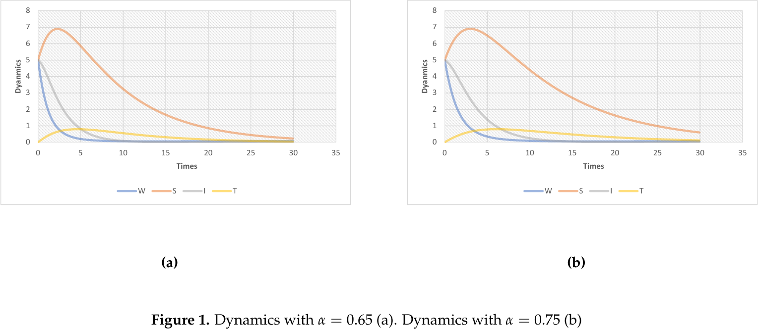
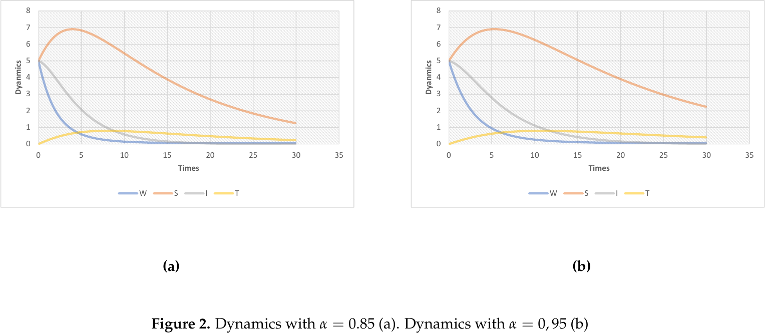
We note that the number of polluted water sources, \(WSs\), may initially be high, then decay or stabilize. The number of WSs susceptible to pollution increases until it reaches a maximum, then decreases as the number of \(WSs\) infected by water pollution (WP) spreads. The number of \(WSs\) infected by water pollution (WP) falls as recovery or treatment occurs. The number of \(WSs\) recovered due to treatment (insoluble class) rises, then decays as treated recover. This also explains the value of the pollution number given by the form that \[ R_{0}=\frac{0.03\times0.005 }{0.05(0.1\times0.03+0.1+0.02 + 0.05)}=0.01734.\tag{50}\]

The conclusion is that the pollution will not persist, as the value is very low and less than 1. The pollution will not persist, and the government will adopt this approach to combat pollution in the water source. The pertinent question is how to control the pollution and whether it persists. In this case, we modify the recruitment rate of new water sources (\(\Lambda\)) and increase \(\rho\), the fraction of infected sources that contribute to new pollution. We also studied the sensitivity of the pollution number to \(\mu\), the natural removal rate of water sources. We set the following values \(\Lambda=0,1\); \(\alpha_{1}=0.02\); \(\alpha_{2}=0.03\); \(\rho=0.2\); \(\mu=0.02\); \(\delta=0.1\); \(\theta_{1}=0.01\); \(\theta_{2}=0.02\); \(\gamma=0.05\); we have the following Figures 3a,3b,4a,4b.

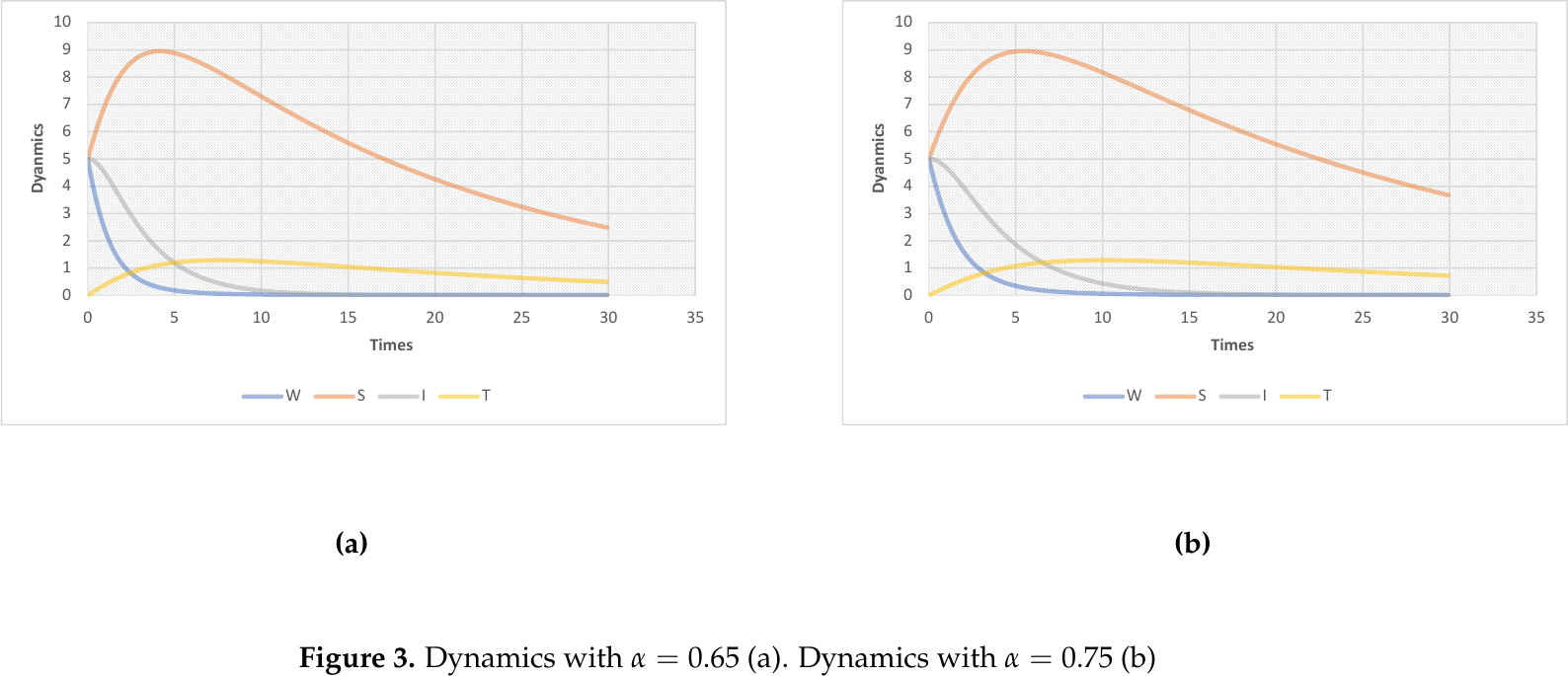
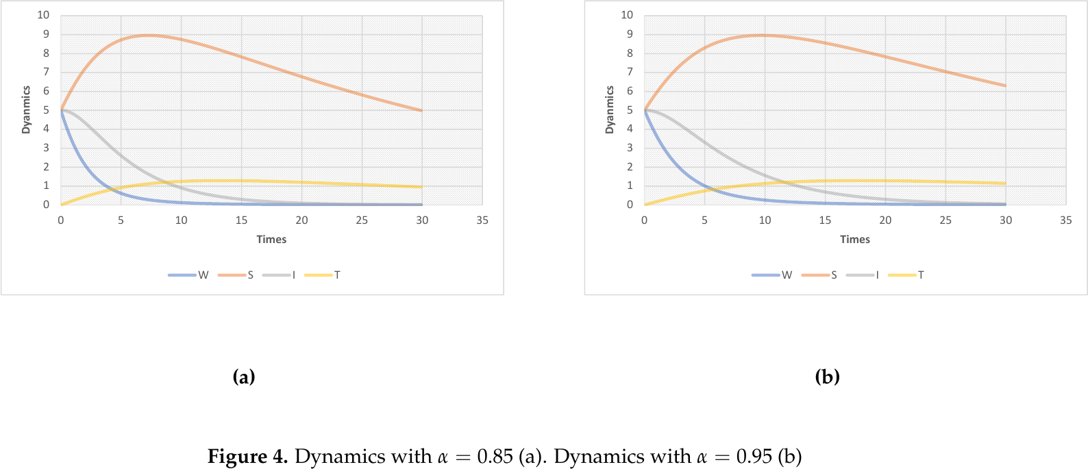
Here, we note changes in the dynamics of our considered model; the novelty is that the behaviors increase or decrease more slowly. We note that the number of polluted water sources, \(WSs\), may initially be high, then decay very slowly, but after a certain time it begins to increase slowly again. The number of WSs susceptible to pollution increases to a maximum, then decreases slowly over time. The number of \(WSs\) recovered due to treatment (insoluble class) rises, then continues to increase as treated recover. Finally, we observe that the number of \(WSs\) infected by water pollution (WP) continues to decrease after its initial value. In the present case, the pollution number also becomes \[ R_{0}=\frac{0.03\times0.1 }{0.02(0.2\times0.03+0.1+0.02 + 0.02)}=1.027.\tag{51}\]

The pollution number \(R_{0} = 1.027>1\). We have observed that an increase in the fraction of infected sources contributing to new pollution and the reduction of \(\mu\), the natural removal rate of water sources, caused pollution to persist. This can be explained by the pollution number being highly sensitive to the pollution number, as observed by taking its derivative with respect to \(\mu\). Therefore, the recommendation is to reduce this number if the government wants to stop water pollution. The influence of the order of the fractional derivative can be observed in the graphics. In general, increasing the order of the fractional derivative does not affect the pollution number. Still, the behaviors, in other words, the increase or the decrease, are retarded when the order increases. We note the retardation effect. For example, when we take the number of WSs susceptible to pollution, it gets its maximum value before \(t=5\) at order \(\alpha=0.65\), see 3a, but when the order is \(\alpha=0.75\), the maximum value is attained after \(t=5\), see Figure 3b. Clearly, the order of the fractional derivative affects the behavior.

5. Optimal control problem

In this section, we propose a control strategy to combat water pollution, a feature that is particularly important for the present model. In our new model, we introduce two types of control, \(u_{1}\), representing sanitation and water treatment. Its utility is to reduce the number of polluted water sources (WSs) and the rates \(\alpha_{1}\) and \(\alpha_{2}\). We also introduce the second control term \(u_{2}\), whose utility is to increase the rate \(\gamma\) and to reduce the transition from \(S\) to \(I\). The model under consideration is given in the form that \[\begin{aligned} \begin{cases} D^{\alpha} W= \Lambda – (1-u_{1})\alpha_{1} WS – (1-u_{1})\alpha_{2} WI + \rho \alpha_{2} I – (\mu + u_{1}) W\\ D^{\alpha} S= (1-u_{1})\alpha_{1} WS + \delta I – (\theta_{1} + \mu) S+ \gamma T\\ D^{\alpha} I= (1-u_{1})\alpha_{2} WI- \rho \alpha_{2} I – (\delta + \theta_{2} + \mu + u_{2})I \\ D^{\alpha} T=\theta_{1} S+ (\theta_{2} + u_{2}) I – (\mu + \gamma) T,\end{cases} \end{aligned}\tag{52}\] with initial conditions defined by the following relationship \[ W(0)=W_0\geq 0, \qquad S(0)=S_0\geq 0, \qquad I(0)=I_0\geq 0, \qquad T(0)=T_0\geq 0.\tag{53}\]

The objective is to minimize the cost function, which includes the total numbers of \(W\) and \(I\) in the water pollution model, as well as the economic costs of the controls \(u_{1}\) and \(u_{2}\). We have the following function \[ \min_{u_{1}, u_{2}(\cdot)\in \ \mathcal U} J(u_{1}, u_{2})=\min_{u_{1}, u_{2}(\cdot)\in \ \mathcal U} \int^{T_{f}}_{0} \left[ aW^{2} + bI^{2} + \frac{1}{2} cu^{2}_{1} + \frac{1}{2} du^{2}_{2}\right] dt,\tag{54}\] where \(a,b,c\), and \(d\) represent weight constants. The constant \(a\) influences the number of polluted water sources, and the weight constant \(b\) affects the number of \(WSs\) infected by water pollution. The constants \(c\) and \(d\) influence the control term, or the cost of the interventions, which is necessary in the calculations. The measurable set \(\mathcal{U}\) of admissible controls is defined as follows \[ \mathcal U = \left\{ (u_{1}, u_{2}), \in L^{1}(0,T_{f}) \mbox{ : } u_{1}(t) \in [0,u_{1,max}]\ , u_{2}(t) \in [0,u_{2,max}]\ \forall \ t \in [0,T_{f}] \right\}.\tag{55}\]

The control problem is well-defined because the cost function is convex (a quadratic form) and we work in a compact set, so we can obtain the minimum or maximum value for the considered control problem. To solve this problem, we use the fractional Pontryagin’s Maximum Principle. The form gives the Hamiltonian function of the problem under consideration. \[\begin{aligned} H(W, S, I, T, u_{1}, u_{2}, \lambda) =& aW^{2} + bI^{2} + \frac{1}{2} cu^{2}_{1} + \frac{1}{2} du^{2}_{2} \\ &+ \lambda_{1} \left[ \Lambda – (1-u_{1})\alpha_1 WS – (1-u_{1})\alpha_{2} WI + \rho \alpha_{2} I – (\mu + u_{1}) W \right] \\ &+ \lambda_{2} \left[ (1-u_{1})\alpha_{1} WS + \delta I – (\theta_{1} + \mu) S + \gamma T \right] \\ &+ \lambda_{3} \left[ (1-u_{1})\alpha_{2} WI – \rho \alpha_{2} I – (\delta + \theta_{2} + \mu + u_{2}) I \right] \\ &+ \lambda_{4} \left[ \theta_{1} S + (\theta_{2} + u_{2}) I – (\mu + \gamma) T \right]. \end{aligned}\]

The adjoint equations are described by the following form, using the Riemann-Liouville derivative, as in the literature on fractional calculus. Using the Hamiltonian function \(H\), we have to solve the following equations with respect to each state variable \[ D^\alpha \lambda_{1}= -\frac{\partial H}{\partial W}, \quad D^\alpha \lambda_{2} = -\frac{\partial H}{\partial S}, \quad D^\alpha \lambda_{3} = -\frac{\partial H}{\partial I}, \quad D^\alpha \lambda_{4} = -\frac{\partial H}{\partial T}.\tag{56}\]

Using the expression described in the Hamiltonian function \(H\), we get that, related to the first variable \(\lambda_1\), we have the following form \[\begin{aligned} D^\alpha \lambda_{1} =&-2aW + \lambda_{1} \left[ (1 – u_{1} )\alpha_{1} S + (1 – u_{1} )\alpha_{2} I + (\mu + u_{1} ) \right] – \lambda_{2} \left[ (1 – u_{1} )\alpha_{1} S \right] – \lambda_{3} \left[ (1 – u_{1} )\alpha_{2} I \right]. \end{aligned}\]

Related to the second parameter \(\lambda_2\), we have the following relationship \[\begin{aligned} D^\alpha \lambda_{2} =&\lambda_{1} \left[ (1 – u_{1})\alpha_{1} W \right] – \lambda_{2} \left[ (1 – u_{1})\alpha_{1} W – (\theta_{1} + \mu) \right] – \lambda_{4} \theta_{1}. \end{aligned}\]

Related to the third variable \(\lambda_3\), we have the following relationship \[\begin{aligned} D^\alpha \lambda_{3} =&-2bI + \lambda_{1} \left[ (1 – u_{1})\alpha_{2} W – \rho \alpha_{2} \right] – \lambda_{2}\delta \lambda_{3} \left[ (1 – u_{1})\alpha_{2} W – \rho \alpha_{2} – (\delta + \theta_{2} + \mu + u_{2}) \right] – \lambda_{4} (\theta_{2} + u_{2}). \end{aligned}\]

Related to the last parameter \(\lambda_{4}\), we have the following equation \[D^\alpha \lambda_{4}= -\lambda_{2} \gamma + \lambda_{4} (\mu + \gamma).\]

We express the transversality conditions with the final states \(W(T_{f}),\) \(S(T_{f})\), \(I(T_{f})\), \(T(T_{f})\), the boundary conditions at the final time \(T_f\) are described in the following relation: \[ \lambda_{1}(T_{f}) = \lambda_{2}(T_{f}) = \lambda_{3}(T_{f}) = \lambda_{4}(T_{f}) = 0.\tag{57}\]

We now propose the optimal control for our minimization problem and apply the following equations to obtain the optimality conditions using the fractional Pontryagin’s Maximum Principle. We have to solve the following equations: \[ \frac{\partial H}{\partial u_{1}} = 0, \quad \frac{\partial H}{\partial u_{2}} = 0.\tag{58}\]

For the first optimal control related to \(u^{*}_{1}\), we apply the differentiation of the Hamiltonian function with respect to the control \(u_{1}\), and then we obtain the form \[ \frac{\partial H}{\partial u_{1}} = cu_{1}+ \lambda_{1} (\alpha_{1} WS + \alpha_{2} WI – W) – \lambda_{2} (\alpha_{1} WS) – \lambda_{3} (\alpha_{2} WI) = 0.\tag{59}\]

We solve according to \(u_{1}\), and we obtain the relationship described by the form \[\begin{aligned} cu_{1} =& \lambda_{1} (W – \alpha_{1} WS – \alpha_{2} WI) + \lambda_{2} (\alpha_{1} WS) + \lambda_{3} (\alpha_{2} WI)\\ u^{*}_{1} =& \frac{1}{c} \left[ \alpha_{1} WS (\lambda_{2} – \lambda_{1}) + \alpha_{2} WI (\lambda_{3} – \lambda_{1}) +\lambda_{1} W \right]. \end{aligned}\]

The same procedure is done to find the optimal control \(u^{*}_{2}\), and by differentiation, we get the form described as: \[\frac{\partial H}{\partial u_{2}} = du_{2}- \lambda_{3} I + \lambda_{4} I = 0.\]

By solving the previous equation, we get the form described by the following for the control \(u_{2}\): \[du_{2} = I (\lambda_{3} – \lambda_{4})\] \[u^{*}_{2}= \frac{I}{d} (\lambda_{3} – \lambda_{4}).\]

Under the bounded environmental models, by assuming the previous conditions, we mean using condition Eq. (55), the form of the first optimal control for our optimal control problem is described as follows: \[u^{*}_{1} = \max\left(0, \min\left(u_{1,max}, \frac{1}{c} \left[ \alpha_{1} WS (\lambda_{2} – \lambda_{1}) + \alpha_{2} WI (\lambda_{3} – \lambda_{1}) + \lambda_{1} W \right]\right)\right).\]

And for the second optimal control, we have the form described by \[u^{*}_{2} = \max\left(0, \min\left(u_{2,max}, \frac{I}{d} (\lambda_{3} – \lambda_{4})\right)\right).\]

We now provide an interpretation of our optimal control problem based on the results of our investigation. The first control mechanism is most effective when the number of polluted water sources \(W\) is high, and the number of WSs susceptible to pollution \(S\) remains large. Practical interventions include chlorine treatment, filtration, and sewage management, which help reduce the number of polluted water sources. The second control is proportional to the number of WSs infected by water pollution, \(I\), and represents a reactive strategy: as \(I\) increases, more resources are required.

6. Conclusion

In this investigation, we have developed a fractional-order model of water pollution. We have used the Caputo derivative to model memory effects in environmental systems. We have determined the equilibrium points of the fractional system, conducted the stability analysis, and provided the pollution number. Our analysis supports the development of an optimal control framework to mitigate the socio-economic and environmental impacts. Numerical schemes have been provided and implemented by the office to obtain the graphics of the dynamics of the water pollution model. In general, it is noticed that the order of the fractional derivative has a retardation effect on the behavior of the dynamics. It is also noted that manipulating the model parameter plays a significant role in the extinction or persistence of water pollution.