
The usage of different operators, generated by linear methods of summation of Fourier series, is a classical way to firter onedimentional signals [1] and in other methods of its processing [1– 4]. As classical example to do it we may use partial Fourier sums [1] \[\label{eq1} S_{n}(t)=S_{n}(f,t)=\frac{a_{0}}{2} + \sum\limits_{k=1}^{n} {(a_{k} \cos (kt) + b_{k} \sin (kt))}, \tag{1}\] where \(f=f(t)\) is a function, what describes stidying signal, \(a_{k}\) and \(b_{k}\) are Fourier coefficients of this function, Fejér operators [1] \[\label{eq2} \sigma_{n} (t)=\sigma_{n} (f,t)=\frac{1}{n} \sum\limits_{k=0}^{n-1} {S_{k}(t)}, \tag{2}\] and its interpolation analogues. Usage of these operators quarntee a filtration of signals in frequency domain, but effect of its usage may be not enouqh strong, especially in case, when we work with signals with large bandwith. In this work we propose a new operator \(\mu_{n} (t)\), described by formula \[\label{eq3} \mu_{n} (t)=\mu_{n} (f,t)=\frac{1}{n} \sum\limits_{k=1}^{n} {\sigma_{k} (t)}, \tag{3}\] what gives more strong effect as signal filter.
To study (3) as method of signal processing a research is built on two steps. First step is based on representation of (3) as operator and making an interpolation analoque of (3) using this operator. Second step based on fitering a concrete signal with random noise using (2) and (3) and comparison of given results. To do it, Python programming language is used. Two scripts on Python is written. First script is written for generation of a signal with addition of random noise using next code:
import numpy as np
    import pandas as pd
    import matplotlib.pyplot as plt

    from numpy import pi
    from scipy.special import gamma, digamma

    # signal forming
    def f(x : np.ndarray) -> np.ndarray:
    return gamma(np.exp(np.sin(x)+np.cos(2*x)/2))*(np.sin(2*x)-np.cos(3*x)/3)
            + digamma(np.exp(np.sin(3*x)-np.cos(4*x)/4))*(np.sin(4*x)+np.cos(5*x)/5)

    N = int(1e6+1)
    x = np.linspace(0, 2*pi, N)
    y = f(x)

    # addition of random noise
    noise = np.random.normal(0, 1, N)
    y = y + noise

    # plotting of generated signal
    plt.plot(x, y)
    plt.xlabel("time in seconds, t")
    plt.ylabel("Noised signal")
    plt.grid()
    plt.show()

    # saving of generated signal
    data = pd.DataFrame()
    data["signal"] = y
    data.index = x
    data.to_csv("signal.csv")
Second Python script realize a filtration of signal, generated by first script, using (2) and (3) for come other values of parameter \(n\) and visualize result of this filtration. This script realizes next code:
import numpy as np
    import pandas as pd
    import matplotlib.pyplot as plt

    from numpy import pi

    # needed functions
    def fejer_sum(x : np.ndarray, f : np.ndarray, n : int) -> np.ndarray:
        def m_sigma(n : int, k : int) -> float:
            return 1.0 - k/n

        if n<0:
            return zeros(len(x))

        res = np.ones(len(x)) * 0.5 * np.mean(f)
        for k in range(1, n):
            res = res + m_sigma(n, k)*( np.mean(f*np.cos(k*x))
                            *np.cos(k*x)+np.mean(f*np.sin(k*x))*np.sin(k*x) )
        return res/n

    def new_sum(x : np.ndarray, f : np.ndarray, n : int) -> np.ndarray:
        def l_mu(n : int, k : int) -> float:
            def H(N : int):
                return sum([1.0/m for m in range(1, N+1)])

            return k * (H(n)-H(k)) / n

        if n<0:
            return np.zeros(len(x))

        res = np.ones(len(x)) * 0.5 * np.mean(f)
        for k in range(1, n+1):
            res = res + l_mu(n, k)*( np.mean
                                 *np.cos(k*x)+np.mean(f*np.sin(k*x))*np.sin(k*x) )
        return res


    # signal reading and filtering
    data = pd.read_csv("signal.csv")
    data.columns = ["time", "signal"]

    t = data["time"].to_numpy()
    f = data["signal"].to_numpy()
    ns = [5, 10, 15]

    fig, axs = plt.subplots(3, 2)
    for i in range(3):
axs[i, 0].plot(t, fejer_sum(t, f, ns[i]), label="Operator (2), n="+str(ns[i]))
axs[i, 0].grid()
axs[i, 0].legend()

axs[i, 1].plot(t, new_sum(t, f, ns[i]), label="Operator (3), n="+str(ns[i]))
axs[i, 1].grid()
axs[i, 1].legend()
plt.show()
After use of these two scripts a comparison of (2) and (3) as filters of signals is made.
Let describe some propositions about operator (3).
Proposition 1. The operator (3) admits the Fourier multiplier representation \[\label{eq4} \mu_{n} (t)=\mu_{n} (f,t)=\frac{1}{n} \frac{a_{0}}{2} + \sum\limits_{k=1}^{n-1} {\lambda_{n, k} (a_{k}\cos kt + b_{k}\sin kt)}, \tag{4}\] where \(\lambda_{n, k} = \frac{k}{n}(H_{n}-H_{k}),\) and \(H_{n} = \sum\limits_{k=1}^{n} {\frac{1}{k}}.\)
Proof. Let denote \[A_{k}(t) = a_{k}\cos kt + b_{k}\sin kt.\] Now let rewrite a formula (3). \[\begin{aligned} \mu_{n} (t) =& \mu_{n} (f,t) = \frac{1}{n} \sum\limits_{k=1}^{n} {\sigma_{k} (t)}\\ =& \frac{1}{n} \cdot \bigg(\frac{a_{0}}{2} + + \frac{a_{0}}{2} + \frac{1}{2}A_{1} + \frac{a_{0}}{2} + \frac{1}{3}A_{1} + \frac{2}{3}A_{2} + \frac{a_{0}}{2} + \frac{1}{4}A_{1} + \frac{2}{4}A_{2} + \frac{3}{4}A_{3} + \dots \\ &+ \frac{a_{0}}{2} + \frac{1}{n}A_{1} + \frac{2}{n}A_{2} + \dots + \frac{n-1}{n}A_{n-1}\bigg)\\ &= \frac{a_{0}}{2} + \sum\limits_{k=1}^{n-1} {\frac{k}{n}(H_{n}-H_{k})A_{k}} \\ &= \frac{a_{0}}{2} + \sum\limits_{k=1}^{n-1} {\frac{k}{n}(H_{n}-H_{k})(a_{k}\cos kt + b_{k}\sin kt)}. \end{aligned}\]
Proposition proofed. ◻
Proposition 2. The operator (3) may be represented by integral \[\label{eq5} \mu_{n} (t)=\mu_{n} (f,t)=\frac{1}{n} \int_{0}^{2 \pi} {f(u) \frac{n \sin \frac{u-t}{2} – \sin \frac{n(u-t)}{2} \cos \frac{(n+1)(u-t)}{2}}{\sin \frac{u-t}{2} (1- \cos (u-t))} du}. \tag{5}\]
Proof. To prove this proposition, let use a fact, that Fejér operator (2) may be represented by integral \[\sigma_{n}(t)=\frac{1}{2n\pi} \int_{0}^{2\pi} {f(u) \frac{1- \cos (n(u-t))}{1 – \cos (u-t)} du}.\]
If we replace this into (3) and doing some manipulations, we will have next \[\mu_{n} (t)=\mu_{n} (f,t)=\frac{1}{n} \int_{0}^{2 \pi} {f(u) \frac{n-\sum\limits_{k=1}^{n} \cos (k(u-t))}{1- \cos (u-t)} du}.\]
Using the equality \[\sum\limits_{k=1}^{n} \cos kx = \frac{\sin \frac{nx}{2} \cos \frac{(n+1)x}{2}}{\sin \frac{x}{2}},\] and doing some additional manipulations, we will have, that \[\mu_{n} (t)=\mu_{n} (f,t)=\frac{1}{n} \int_{0}^{2 \pi} {f(u) \frac{n \sin \frac{u-t}{2} – \sin \frac{n(u-t)}{2} \cos \frac{(n+1)(u-t)}{2}}{\sin \frac{u-t}{2} (1- \cos (u-t))} du}.\]
Proposition proofed. ◻
Proposition 3. Let consider, that \(K_{n}(t)\) is a kernel of (5). So, \[\frac{1}{\pi} \int_{0}^{2\pi} {K_{n}(t)dt}=1.\] for all natural \(n\).
Proof. After doing some operations with \(K_{n}(t)\), we will see, that \[K_{n} = \frac{1}{2} + \sum\limits_{k=1}^{n-1} {\frac{k}{n}(H_{n}-H_{k})(\cos kt + \sin kt)},\] where \[H_{n} = \sum\limits_{k=1}^{n} {\frac{1}{k}}.\]
Using it, we will have next. \[\begin{aligned} \int_{0}^{2\pi} {K_{n}(t)dt}=& \int_{0}^{2\pi} {\frac{1}{2} + \sum\limits_{k=1}^{n-1} {\frac{k}{n}(H_{n}-H_{k})(\cos kt + \sin kt)}}\\ =& \frac{1}{2} \int_{0}^{2\pi} {dt} + {\frac{k}{n}(H_{n}-H_{k})\left(\int_{0}^{2\pi} {\cos kt dt} + \int_{0}^{2\pi} {\sin kt dt}\right)} \\=& \pi. \end{aligned}\]
As the result, we hill have, that \[\frac{1}{\pi} \int_{0}^{2\pi} {K_{n}(t)dt}=\frac{\pi}{\pi}=1.\]
Proposition proofed. ◻
Proposition 4. Let consider, that \(K_{n}(t)\) is a kernel of (5). So, limit \[\lim_{t \to 0} {K_{n}(t)dt},\] equals \[\frac{1}{2} + \frac{1}{n} \int_{0}^{1} { \frac{\sum\limits_{k=1}^{n-1} {kx^{k}}}{1-x} dx } – \frac{n-1}{2} \int_{0}^{1} {\frac{x^{n}}{1-x} dx},\] and is finit for all finite \(n\).
Proof. As in proof of proposition 3, let use representation of \(K_{n}(t)\) in a form \[K_{n} = \frac{1}{2} + \sum\limits_{k=1}^{n-1} {\frac{k}{n}(H_{n}-H_{k})(\cos kt + \sin kt)},\] where \[H_{n} = \sum\limits_{k=1}^{n} {\frac{1}{k}}.\]
Using it, let find \(\lim_{t \to 0} {K_{n}(t)dt}\). \[\lim_{t \to 0} {K_{n}(t)dt} = \lim_{t \to 0} { \left(\frac{1}{2} + \sum\limits_{k=1}^{n-1} {\frac{k}{n}(H_{n}-H_{k})(\cos kt + \sin kt)}\right) } = \frac{1}{2} + \sum\limits_{k=1}^{n-1} {\frac{k}{n}(H_{n}-H_{k})}.\]
Using an integral representation of harmonic numbers \(H_{n}\) in form \[H_{n} = \int_{0}^{1} {\frac{1-x^{n}}{1-x} dx},\] we will have next \[\begin{aligned} \lim_{t \to 0} {K_{n}(t)dt} =&\frac{1}{2} + \sum\limits_{k=1}^{n-1} { \frac{k}{n} \int_{0}^{1} {\frac{x^{k}-x^{n}}{1-x} dx} }\\ =&\frac{1}{2} + \frac{1}{n}\int_{0}^{1} {\frac{1}{1-x}\left(\sum\limits_{k=1}^{n-1} {kx^{k}}\right) dx} – \frac{1}{n} \left(\sum\limits_{k=1}^{n-1} {k}\right) \int_{0}^{1} {\frac{x^{n}}{1-x} dx}\\ =& \frac{1}{2} + \frac{1}{n} \int_{0}^{1} { \frac{\sum\limits_{k=1}^{n-1} {kx^{k}}}{1-x} dx } – \frac{n-1}{2} \int_{0}^{1} {\frac{x^{n}}{1-x} dx}. \end{aligned}\]
It’s easy to see, that for finite \(n\) an expression \[\frac{1}{2} + \frac{1}{n} \int_{0}^{1} { \frac{\sum\limits_{k=1}^{n-1} {kx^{k}}}{1-x} dx } – \frac{n-1}{2} \int_{0}^{1} {\frac{x^{n}}{1-x} dx},\] is finite too. It may be shown by making one integral from second and third terms in this expression. It may be shown using Bézout’s theorem, that given integral is finite for every finite \(n\).
Proposition prooved. ◻
Let analyze described propositions. Proposition 1 shows, that operator (3) is a triangular linear summation method of Fourier series with multipliers \(\lambda_{n, k}\), which may be calculated by formula \[\lambda_{n, k} = \frac{k}{n}(H_{n}-H_{k}) = \frac{k}{n} \sum\limits_{m=k}^{n} \left( 1-\frac{k}{m+1} \right),\] what is different from the previously described ones. For example, multipliers \(\lambda_{n, k}\) for a Fejér operator may be calculated by formula \[\lambda_{n, k} = 1-\frac{k}{n},\] and for Abel-Poisson partial sums [5] may be calculated by formula \[\lambda_{n, k} = e^{-\frac{k}{n}}.\]
In addition, proposition 1 shows, that operator (3) satisfies the classical conditions of regular linear summation methods: bounded multipliers, convergence of \(\lambda_{n, k}\) to 1 for fixed k when \(n \to \inf\), and preservation of constant functions.
Second proposition 2 allows to write an discrete variant of (5), what in some literature, related with Fourier analysis (for example, in [2] or [5]), is called as interpolation analogue of operator and may be written by formula \[\label{eq6} \tilde{\mu}_{n} (t)=\tilde{\mu}_{n} (f,t)=\frac{1}{mn} \sum\limits_{k=1}^{m} {f(t_{k}) \frac{n \sin \frac{t_{k}-t}{2} – \sin \frac{n(t_{k}-t)}{2} \cos \frac{(n+1)(t_{k}-t)}{2}}{\sin \frac{t_{k}-t}{2} (1- \cos (t_{k}-t))}}, \tag{6}\] where sequence of argument values \(\{t_{k}\}_{k=1}^{m}\) gives an uniform grid in interval [\(0;2\pi\)].
Third and fourth Propositions 3 and 4 are about properties of a kernel of integral representation of operator (3). These propositions say, that integral of this kernel is finite, what may be useful in approximation theory and signal processing, especially, in approximation of digital signals using discrete variant (6).
For demonstration difference of signal filtering using (2) and (3) firstly let compare behavior of Fourier coefficient multipliers of these operators. To do it, let denote Fourier coefficient multipliers for Fejér operators (2) as \[\lambda_{\sigma_{n}} (n, k) = 1 – \frac{k}{n},\] and Fourier coefficient multipliers for operator (3) as \[\lambda_{\mu_{n}} (n, k) = \frac{k}{n} (H_{n} – H_{k}).\]
Now let visualize \(\lambda_{\sigma_{n}} (n, k)\) and \(\lambda_{\mu_{n}} (n, k)\) for some different values of parameter \(n\).
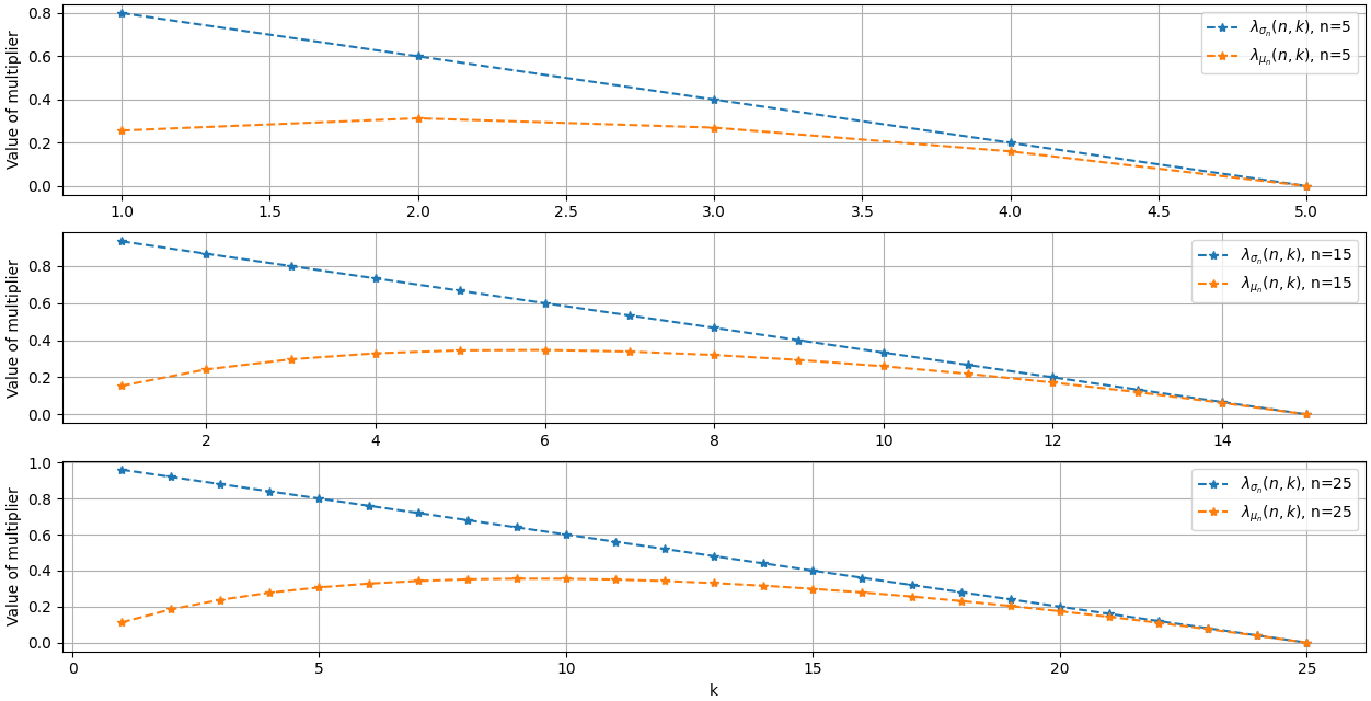
As we may see on Figure 1, the introduced operator (3) may give really stronger frequency suppression than Fejér operator (2), but this suppression has other behavior: unlike Fejér operator \(\sigma_{n} (t)\) operator \(\mu_{n} (t)\) will supress all harmonics, but the further harmonics is from \(\lfloor \frac{n}{3} \rfloor + 1\)-th, a more suppression of this harmonics will be expected. This factor may be used for signal filtering, especially in case of localization needed frequency.
To demonstrate described effect let consider a digital signal, continious equivalent of which may be described by function \[f(t)=\Gamma \left(e^{\sin t + \frac{\cos 2t}{2}}\right)\left(\sin 2t – \frac{\cos 3t}{3}\right) + \psi \left(e^{\sin 3t – \frac{\cos 4t}{4}}\right)\left(\sin 4t + \frac{\cos 5t}{5}\right), t \in [0, 2\pi].\] and let add to every \(i\)-th sample of signal and additive white Gaussian noise \(\nu_{i} \sim N(0, 1)\).
Firstly, let visualize noised signal.
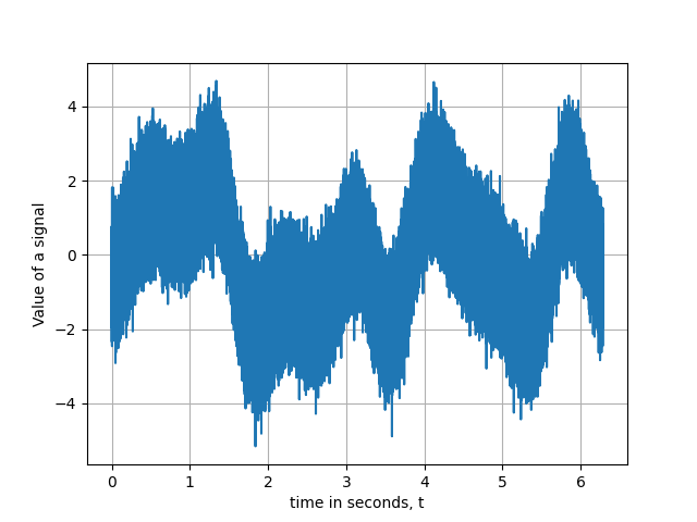
Now, let visualize a result of firtering of signal, shown on Figure 2, using (2) and (3) with different values of parameter \(n\).
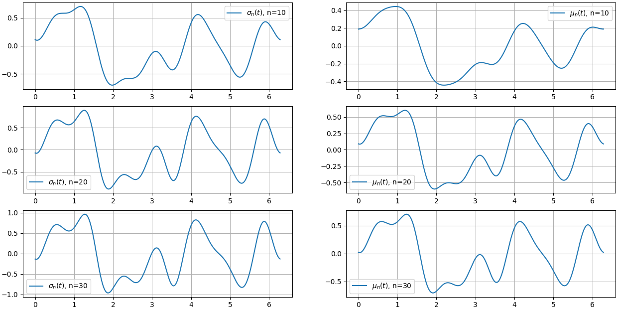
We see, that visually interpolation analogues of (3) may be used as signal filter and as approximator of digital signals like interpolation analogues of Fejér operators (2), but in case of small values of parameter \(n\) looks worth. But, as we may see on Figure 3, it may be solved by using of higher values of \(n\).
To make more detailed research of an effect of approximation of the signal using interpolation analogues of (2) and (3) let visualize a dependence between mean squared error \[MSE = \frac{1}{N} \sum\limits_{k=1}^{N} ( f(t_{k}) – \tilde{f}(t_{k}) )^{2},\] (between real digital signal \(f(t_{k})\) and result of usage of interpolation analoque \(\tilde{f}(t_{k})\) of (2) and (3)) and value of parameter \(n\).
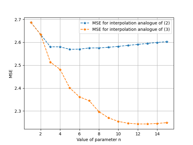
On Figure 4 we may see, that in case of \(n>2\) interpolation analogues of (3) may give less MSE, what means, that for same values of parameter \(n\) and sample rate interpolation analogues of operator \(\mu_{n} (t)\) gives better approximation of digital signal, than interpolation analogues of Fejér operator \(\sigma_{n} (t)\).
This research is considering operator \(\mu_{n} (f, t)\), defined by formula (3). As a research shows, this operator has an intergal representation (5). Discrete form (6) of this integral representation, what sometimes is called interpilation analogue of an operator, may be used for approximation of one-dimentional digital signal in time domain, what may be seen on Figure 2 and Figure 3, but this approximation will be better, that approximation using interpolation analogue of Fejér operator in case of same value of parameter \(n\) and same sampling rate, what we may see on Figure 4. In addition, research shows, that operator (3) admits the Fourier multiplier representation, what was demonstrated and proofed as one of propositions.
These aspects may have practical value in DSP. For example, in future research approximation properties of (3) may be studied and compared with approximation properties of other, windly used operators like Fejér operator (2) [1], Abel-Poisson operators [2] and its triangular analogue [5] or other. As other perspective of future research interpolation analogue (6) may be studied and compared with other interpolation methods [7– 9], especially, in case of DSP [10, 11]. In addition, future research may be based on studying of (6) as a numerical method [12]. As existing research shows, (6) may be considered in context of modeling [13, 14], fundamental research of approximation and filtering methods [1, 16] and many other aspects of DSP.