
With the continuous development of financial derivatives markets, option products have increasingly expanded their roles in risk management, return enhancement, and asset allocation. Compared with standard European options whose payoffs depend solely on the underlying asset price at maturity, an increasing number of complex derivatives incorporate path dependent features, making option values depend not only on terminal states but also on the price evolution of the underlying asset over the entire life of the contract [1]. In this context, lock-in options, also referred to as shout options, permit holders to secure partial or full payoffs in advance during the life of the contract and have therefore attracted growing attention in both academic research and practical applications [2]. The core feature of lock-in options lies in allowing the holder, at one or multiple points prior to maturity, to confirm future payoffs in advance based on market conditions, thereby effectively reducing downside risk without fully sacrificing subsequent upside potential [3]. Among various lock-in options, active lock-in options grant the holder the right to independently choose the lock-in timing at any moment prior to maturity, making the payoff structure depend jointly on the underlying asset prices at the lock-in time and at maturity. This mechanism confers upon such options the dual characteristics of early payoff locking and continued participation in market fluctuations, which makes them especially appealing in the design of structured wealth management products, insurance linked derivatives, and capital protected financial instruments [4].
However, precisely because active lock-in options introduce path dependence and dynamic decision mechanisms, their pricing problems are mathematically significantly more complex than those of standard options, as option values depend not only on terminal prices but also on the entire price evolution path of the underlying asset and the choice of optimal lock-in timing.
In existing studies, reliance on the deterministic volatility assumption of the Black Scholes Merton framework often fails to capture market phenomena such as implied volatility smiles, volatility clustering, and changes in volatility term structures, resulting in systematic deviations between theoretical prices and market observations [5]. Therefore, incorporating stochastic volatility models into lock-in option pricing, so as to more realistically characterize uncertainty in underlying asset prices, is of significant theoretical importance and practical value. Against this background, this paper systematically investigates the pricing of active lock-in options under stochastic volatility environments, aiming to characterize their value structure and optimal lock-in decision mechanisms within modeling frameworks that more closely reflect real market characteristics. Such research not only deepens theoretical understanding of optimal decision making in path dependent options but also provides reliable theoretical foundations and numerical tools for the pricing and risk management of complex structured derivatives in real financial markets.
The Heston stochastic volatility model [6] introduces a mean reverting square root diffusion to describe the stochastic dynamics of variance, allowing the asset return volatility to evolve randomly over time while exhibiting long-run mean reversion.
Under the risk neutral measure \(\mathbb{Q}\), the dynamics of the asset price \(X_t\) and the instantaneous variance \(z_t\) are given by \[ \frac{dX_t}{X_t} = r\,dt + \sqrt{z_t}\,dW_t^{X}, \label{eq:heston_price} \ \tag{1}\] \[dz_t = \kappa(\theta – z_t)\,dt + \sigma_z \sqrt{z_t}\,dW_t^{z}, \label{eq:heston_var} \tag{2}\] where \(r\) denotes the constant risk free interest rate and \(W_t^{X}\) and \(W_t^{z}\) are standard Brownian motions defined on a filtered probability space.
The parameters satisfy \(\kappa>0\), \(\theta>0\), and \(\sigma_z>0\), with initial variance \(z_0>0\). Here, \(\kappa\) represents the speed of mean reversion of the variance process, \(\theta\) is the long-run variance level, and \(\sigma_z\) controls the volatility of variance.
To ensure strict positivity of the variance process and avoid degeneracy of the diffusion term, the model is commonly assumed to satisfy the Feller condition \[2\kappa\theta \ge \sigma_z^{2}. \tag{3}\]
Let the option maturity be denoted by \(T\), and define the remaining time to maturity as \(\tau = T – t\).
In the contract structure of an active lock-in call option, the holder is allowed to choose a single lock-in time \(t^{*}\) at any point within the interval \([0,T]\) and execute the lock-in operation. Upon execution of the lock-in, the option immediately realizes its intrinsic value \((S_{t^{*}}-K)^{+}\), while the original contract is reset to a European call option with remaining maturity \(\tau = T – t^{*}\) and strike price set equal to the prevailing asset price, namely \(K' = S_{t^{*}}\). After the lock-in, the holder continues to hold this at the money (ATM) European call option until maturity.
From the perspective of terminal payoff, if the lock-in is executed at time \(t^{*}\) and \(S_{t^{*}}=S\), the total payoff of the active lock-in call option at maturity \(T\) can be written as \[\Pi_T = \max\bigl(S_T – K,\; S – K,\; 0\bigr). \tag{4}\]
Using the identity \(\max(x,c)=c+(x-c)^{+}\) for \(c\ge0\), the terminal payoff admits the equivalent decomposition \[\Pi_T = (S-K)^{+} + (S_T – S)^{+}. \tag{5}\]
This decomposition shows that a single lock-in operation is financially equivalent to the combination of two payoff components: the intrinsic value \((S_{t^{*}}-K)^{+}\) realized immediately at the lock-in time, and the random terminal payoff \((S_T-S_{t^{*}})^{+}\) of a European call option with strike price \(K'=S_{t^{*}}\).
This chapter develops a pricing model for active lock-in options under a stochastic volatility environment within a continuous time financial market framework.
By characterizing the joint dynamics of the underlying asset price and volatility and explicitly specifying the payoff structure induced by the active lock-in mechanism, the pricing problem is rigorously formulated as a free boundary problem with optimal stopping features, thereby laying the foundation for subsequent theoretical analysis and numerical solution.
Under the risk neutral measure \(\mathbb{Q}\), the underlying asset price process \(\{S_t\}_{t\ge 0}\) and its variance process \(\{v_t\}_{t\ge 0}\) are described by the classical Heston stochastic volatility model, whose dynamics satisfy the following system of stochastic differential equations. \[\left\{\begin{aligned} \frac{dS_t}{S_t} &= r\,dt + \sqrt{v_t}\,dW_t^{(1)}, \\ dv_t &= \kappa(\theta – v_t)\,dt + \xi \sqrt{v_t}\,dW_t^{(2)}, \end{aligned} \qquad\qquad d\langle W^{(1)}, W^{(2)} \rangle_t = \rho\,dt.\right. \label{eq:heston} \tag{6}\]
Here, \(r\) denotes the constant risk free interest rate, \(\kappa>0\) is the speed of mean reversion of the variance process, \(\theta>0\) is the long run variance level, \(\xi>0\) represents the volatility of variance parameter, and \(\rho\in[-1,1]\) is the correlation coefficient between the asset price and variance processes. Let the option maturity be \(T\), and define the remaining time to maturity as \(\tau=T-t\), with \(u(S,v,\tau)\) denoting the option value function at the current state \((S,v,\tau)\).
Based on the payoff decomposition in §2.2, an immediate lock-in at state \((S,v,\tau)\) yields \[\phi(S,v,\tau) =(S-K)^{+}+C_{\mathrm{Eur}}(S,K'=S,v,\tau), \label{eq:obstacle_function} \tag{7}\] which serves as the obstacle in the associated optimal stopping problem, the European call price admits the semi closed form \[C_{\mathrm{Eur}}(S,K,v,\tau) = S\,P_1(S,K,v,\tau)\;-\;K e^{-r\tau}\,P_2(S,K,v,\tau), \label{eq:heston_call_SK} \tag{8}\] the terms \(P_j\), \(j=1,2\), are given by the standard Heston probability representations, \[P_j(S,K,v,\tau) =\frac{1}{2} +\frac{1}{\pi}\int_{0}^{\infty} \Re\!\left( \frac{e^{-iu\ln(K/S)}\,\Psi_j(u;v,\tau)}{iu} \right)\,du, \qquad j=1,2, \label{eq:Pj_heston_SK} \tag{9}\] where \(\Psi_j(u;v,\tau)\) are functions derived from the Heston characteristic function.
For the lock-in continuation value, the strike is reset to \(K'=S\), hence \[C_{\mathrm{Eur}}(S,K'=S,v,\tau) = S\left(P_1(S,S,v,\tau)-e^{-r\tau}P_2(S,S,v,\tau)\right). \label{eq:reset_call_SK} \tag{10}\]
Substituting (10) into (7) yields the compact obstacle \[\phi(S,v,\tau) =(S-K)^{+}+S\left(P_1(S,S,v,\tau)-e^{-r\tau}P_2(S,S,v,\tau)\right). \label{eq:obstacle_compact_SK} \tag{11}\]
Based on the preceding model specification, the value function of the active lock-in call option can naturally be formulated as an optimal stopping problem.Specifically, under the risk neutral measure \(\mathbb{Q}\), the option value can be expressed as \[u(S,v,\tau) = \sup_{\tau^* \in [0,\tau]} \mathbb{E}^{\mathbb{Q}} \left[ (S_{\tau^*}-K)^+ + C_{\mathrm{Eur}} \left(S_{\tau^*}, K'=S_{\tau^*}, v_{\tau^*}, \tau-\tau^*\right) \right]. \label{eq:optimal_stopping} \tag{12}\]
Here, \(\tau^*\) denotes the admissible lock-in time, the first term represents the intrinsic value realized immediately upon lock-in, and the second term corresponds to the value of the at the money European call option held after the lock-in.
For any sufficiently smooth function \(f(S,v)\), the infinitesimal generator \(L\) associated with the Heston stochastic volatility model [7] is defined as \[L f = r S f_S + \kappa(\theta – v) f_v + \frac{1}{2} v S^2 f_{SS} + \rho \xi v S f_{Sv} + \frac{1}{2} \xi^2 v f_{vv}. \label{eq:heston_generator} \tag{13}\]
In the continuation region (i.e., where \(u>\phi\)), the option value function satisfies the following partial differential equation according to the risk neutral pricing principle. \[\partial_\tau u = L u – r u, \qquad u > \phi, \label{eq:continuation_pde} \tag{14}\]
Here, \(\phi(S,v,\tau)\) denotes the payoff function corresponding to immediate execution of the lock-in operation.
The terminal condition corresponds to the option value at zero remaining maturity, namely the instantaneous payoff of an at the money European call option. \[u(S,v,0) = (S-K)^+. \label{eq:terminal_condition} \tag{15}\]
To align the analytical formulation with the numerical discretization, we work in the log moneyness variable \[x=\ln\!\left(\frac{S}{K}\right), \qquad S = K e^{x}, \label{eq:log_moneyness} \tag{16}\] and define the transformed value function \[U(x,v,\tau) := u(Ke^{x},v,\tau). \label{eq:U_def} \tag{17}\]
Accordingly, we also express the obstacle in \((x,v)\) coordinates as \[\Phi(x,v,\tau):=\phi(Ke^{x},v,\tau). \label{eq:Phi_def} \tag{18}\]
By the chain rule, the derivatives of \(u(S,v,\tau)\) with respect to \((S,v)\) can be expressed in terms of derivatives of \(U(x,v,\tau)\) as \[u_S = \frac{1}{S}U_x, \qquad u_{SS} = \frac{1}{S^2}\bigl(U_{xx}-U_x\bigr), \qquad u_v = U_v, \qquad u_{Sv} = \frac{1}{S}U_{xv}. \label{eq:derivative_transform} \tag{19}\]
Substituting (19) into the Heston generator in \((S,v)\) yields the infinitesimal generator in the variables \((x,v)\): \[\mathcal{L}^{(x,v)}U = \frac{1}{2}v\,U_{xx} +\rho \xi v\,U_{xv} +\frac{1}{2}\xi^2 v\,U_{vv} +\left(r-\frac{1}{2}v\right)U_x +\kappa(\theta-v)U_v. \label{eq:generator_xv} \tag{20}\]
In the continuation region, the value function satisfies: \[\partial_\tau U(x,v,\tau) = \mathcal{L}^{(x,v)}U(x,v,\tau) – r\,U(x,v,\tau), \qquad U(x,v,\tau)>\Phi(x,v,\tau). \label{eq:pde_continuation_xv} \tag{21}\]
The terminal condition at \(\tau=0\) is inherited from the payoff: \[U(x,v,0)=u(Ke^{x},v,0)=(Ke^{x}-K)^+. \label{eq:terminal_xv} \tag{22}\]
By combining the PDE (21) in the continuation region with the immediate lock-in condition \(U=\Phi\), the pricing problem of the active lock-in call option can be equivalently formulated as a standard Linear Complementarity Problem (LCP). \[\left\{ \begin{aligned} & U(x,v,\tau) \ge \Phi(x,v,\tau), \\[4pt] & \partial_{\tau} U – \mathcal{L}^{(x,v)}U + r U \ge 0, \\[4pt] & \bigl(U – \Phi\bigr)\, \bigl(\partial_{\tau} U – \mathcal{L}^{(x,v)}U + r U\bigr) = 0, \end{aligned} \right. \tag{23}\]
Here, \(x\in\mathbb{R}\), \(v\ge 0\), and \(\tau\in(0,T)\).
These complementarity conditions characterize the optimal switching mechanism between the continuation region and the active lock-in region: when immediate lock-in is optimal, the option value satisfies \(U=\Phi\); otherwise, in the continuation optimal case, the value function satisfies the corresponding partial differential equation, thereby providing the theoretical foundation for subsequent numerical solution methods.
In the previous section, the pricing problem of the active lock-in call option was formulated as a linear complementarity problem with obstacle constraints. Building on this formulation, this section further develops the corresponding numerical solution methods.
Within the continuation region, the option value function satisfies \[\partial_\tau U(x,v,\tau) = \mathcal{L}^{(x,v)}U(x,v,\tau) – r\,U(x,v,\tau), \qquad U(x,v,\tau)>\Phi(x,v,\tau), \label{eq:pde_continuation_xv_imex} \tag{24}\] where \(\Phi(x,v,\tau)\) is the obstacle and the infinitesimal generator \(\mathcal{L}^{(x,v)}\) is given in (20). A fully implicit treatment of the mixed-derivative term \(\rho\,\xi\,v\,U_{xv}\) may deteriorate the monotonicity properties of the discrete operator. We therefore employ an IMEX discretization in which the unmixed diffusion terms are handled implicitly, while the mixed derivative and drift terms are treated explicitly.
We separate the spatial operator into an implicit and an explicit component, \[\mathcal{L}^{(x,v)}U – rU = \mathcal{L}_{\mathrm{imp}}U + \mathcal{L}_{\mathrm{exp}}U, \label{eq:imex_split_no_beta_cont} \tag{25}\] with \[ \mathcal{L}_{\mathrm{imp}}U = \frac{1}{2}v\,U_{xx} +\frac{1}{2}\xi^2 v\,U_{vv}, \label{eq:Limp_no_beta_cont}\ \tag{26}\] \[\mathcal{L}_{\mathrm{exp}}U = \rho\,\xi\,v\,U_{xv} +\Bigl(r-\frac{1}{2}v\Bigr)U_x +\kappa(\theta-v)U_v -rU. \label{eq:Lexp_no_beta_cont} \tag{27}\]
Let \(\{x_i\}_{i=0}^{N_x}\) and \(\{v_j\}_{j=0}^{N_v}\) be a tensor grid in \((x,v)\) and let \(\mathbf{U}(\tau)\) collect the nodal values \(\{U(x_i,v_j,\tau)\}\) in a fixed ordering. We denote by \(\mathcal{L}_{\mathrm{imp},h}\) and \(\mathcal{L}_{\mathrm{exp},h}\) finite difference approximations of \(\mathcal{L}_{\mathrm{imp}}\) and \(\mathcal{L}_{\mathrm{exp}}\), respectively, so that \[\frac{d}{d\tau}\mathbf{U}(\tau) = \mathcal{L}_{\mathrm{imp},h}\,\mathbf{U}(\tau) + \mathcal{L}_{\mathrm{exp},h}\,\mathbf{U}(\tau). \label{eq:semi_discrete_split_no_beta} \tag{28}\]
In terms of difference operators, we implement \[ \mathcal{L}_{\mathrm{imp},h}\mathbf{U} := \frac{1}{2}\,\mathrm{diag}(v)\,\delta_{xx}\mathbf{U} +\frac{1}{2}\xi^2\,\mathrm{diag}(v)\,\delta_{vv}\mathbf{U}, \label{eq:Limp_h_no_beta}\ \tag{29}\] \[\mathcal{L}_{\mathrm{exp},h}\mathbf{U} := \rho\,\xi\,\mathrm{diag}(v)\,\delta_{xv}\mathbf{U} +\mathrm{diag}\!\Bigl(r-\tfrac{1}{2}v\Bigr)\,\delta_x\mathbf{U} +\mathrm{diag}\!\bigl(\kappa(\theta-v)\bigr)\,\delta_v\mathbf{U} -r\,\mathbf{U}, \label{eq:Lexp_h_no_beta} \tag{30}\] where \(\delta_{xx}\) and \(\delta_{vv}\) are second order difference operators, \(\delta_{xv}\) is the mixed derivative stencil, and \(\delta_x,\delta_v\) are first order difference operators.
On a uniform tensor grid \(x_i=x_{\min}+i\Delta x\) (\(i=0,\dots,N_x\)) and \(v_j=j\Delta v\) (\(j=0,\dots,N_v\)), we approximate the second-order unmixed diffusion terms by standard centered differences, \[ (\delta_{xx}U)_{i,j} := \frac{U_{i+1,j}-2U_{i,j}+U_{i-1,j}}{\Delta x^2}, \qquad 1\le i\le N_x-1, \label{eq:fd_dxx}\ \tag{31}\] \[(\delta_{vv}U)_{i,j} := \frac{U_{i,j+1}-2U_{i,j}+U_{i,j-1}}{\Delta v^2}, \qquad 1\le j\le N_v-1, \label{eq:fd_dvv} \tag{32}\] and the mixed derivative is discretized by the standard 4-point cross stencil, \[\begin{aligned} (\delta_{xv}U)_{i,j} &:= \frac{U_{i+1,j+1}-U_{i+1,j-1}-U_{i-1,j+1}+U_{i-1,j-1}}{4\,\Delta x\,\Delta v},\\ &\qquad 1\le i\le N_x-1,\quad 1\le j\le N_v-1. \end{aligned} \label{eq:mixed_cross_stencil} \tag{33}\]
In the numerical implementation, we truncate the state space to \(x\in[x_{\min},x_{\max}]\) and \(v\in[0,v_{\max}]\), where \(x_{\min}\) is set so that \(S=Ke^{x_{\min}}\) is deep out of the money, \(x_{\max}\) lies in a region where the solution is well approximated by the obstacle, and \(v_{\max}\) is chosen such that \(\mathbb{P}\!\left(\sup_{t\in[0,T]} v_t>v_{\max}\right)\) is negligible under the Heston dynamics.
At the truncated asset boundaries we impose Dirichlet conditions \[\begin{aligned} U(x_{\min},v,\tau) &= 0,\\ U(x_{\max},v,\tau) &= \Phi(x_{\max},v,\tau), \end{aligned} \qquad v\in[0,v_{\max}],\ \tau\in[0,T], \label{eq:bc_dirichlet_x} \tag{34}\] and enforce them by row replacement in the linear system. Along the variance boundaries we impose Neumann conditions, \[\left\{\begin{aligned} \partial_v U(x,0,\tau) &= 0,\\ \partial_v U(x,v_{\max},\tau) &= 0, \end{aligned} \qquad\qquad x\in[x_{\min},x_{\max}],\ \tau\in[0,T],\right. \label{eq:bc_neumann_v} \tag{35}\] which are robust for the degenerate limit \(v\downarrow 0\) and are justified at \(v=v_{\max}\) by choosing \(v_{\max}\) sufficiently large so that the solution is nearly flat in \(v\) near the boundary. Along the variance boundaries we enforce a Neumann condition \(U_v(x,0,\tau)=U_v(x,v_{\max},\tau)=0\), which can be implemented via ghost point reflection, e.g. \(U_{i,-1}=U_{i,1}\) at \(v=0\) and \(U_{i,N_v+1}=U_{i,N_v-1}\) at \(v=v_{\max}\), yielding the one sided second derivative approximations \[(\delta_{vv}U)_{i,0}=\frac{2(U_{i,1}-U_{i,0})}{\Delta v^2},\qquad (\delta_{vv}U)_{i,N_v}=\frac{2(U_{i,N_v-1}-U_{i,N_v})}{\Delta v^2}. \tag{36}\]
Let \(\Delta\tau>0\) be the time step and \(\tau_m=m\Delta\tau\), \(m=0,1,\dots,M\). The IMEX Euler step in the continuation region reads \[\frac{\mathbf{U}^{m}-\mathbf{U}^{m-1}}{\Delta\tau} = \mathcal{L}_{\mathrm{imp},h}\mathbf{U}^{m} + \mathcal{L}_{\mathrm{exp},h}\mathbf{U}^{m-1}, \qquad m=1,2,\dots,M, \label{eq:imex_euler_split_no_beta} \tag{37}\] or equivalently, \[\underbrace{\bigl(I-\Delta\tau\,\mathcal{L}_{\mathrm{imp},h}\bigr)}_{=:A}\mathbf{U}^{m} = \underbrace{\mathbf{U}^{m-1} +\Delta\tau\,\mathcal{L}_{\mathrm{exp},h}\mathbf{U}^{m-1}}_{=:\mathbf{b}^{m}}, \label{eq:imex_linear_no_beta} \tag{38}\] where diffusion is treated implicitly to alleviate stiffness, while drift, discount and the mixed derivative are treated explicitly.
Let \(\boldsymbol{\Phi}^{m}\) denote the obstacle sampled at \(\tau_m\). The lock-in feature imposes the componentwise constraint \(\mathbf{U}^{m}\ge \boldsymbol{\Phi}^{m}\). Combining this with (38) yields the standard discrete linear complementarity problem (LCP): \[\mathbf{U}^{m}\ge \boldsymbol{\Phi}^{m},\quad A\mathbf{U}^{m}\ge \mathbf{b}^{m},\quad (\mathbf{U}^{m}-\boldsymbol{\Phi}^{m})\odot(A\mathbf{U}^{m}-\mathbf{b}^{m})=\mathbf{0}, \label{eq:lcp_discrete} \tag{39}\] where \(\odot\) denotes the Hadamard product. Finally, the lock-in feature can be expressed in the continuous form as \[\min\bigl\{U-\Phi,\ \partial_\tau U-\mathcal{L}U+rU\bigr\}=0, \tag{40}\] thereby defining the lock-in region and the associated free boundary.
Proposition 1(Nonsingular \(M\)-matrix property of \(A\)).Let \(A:=I-\Delta\tau\,\mathcal{L}_{\mathrm{imp},h}\), where \[\mathcal{L}_{\mathrm{imp},h} =\tfrac12\,\mathrm{diag}(v)\,\delta_{xx} +\tfrac12\,\xi^2\,\mathrm{diag}(v)\,\delta_{vv}.\]
Assume Dirichlet conditions in \(x\) are enforced by row replacement and the variance boundaries \(v=0\) and \(v=v_{\max}\) are closed by Neumann discretization. Then \(A\) is a nonsingular \(M\)-matrix: it is a \(Z\)-matrix and satisfies \(A^{-1}\ge 0\) componentwise.
Proof. (i) \(A\) is a \(Z\)-matrix.
On interior nodes, \(\mathcal{L}_{\mathrm{imp},h}\) contains only centered second differences. Since \(v_j\ge 0\), the resulting couplings to nearest neighbors in \(A=I-\Delta\tau\,\mathcal{L}_{\mathrm{imp},h}\) have coefficients \(-\Delta\tau\,c\) with \(c\ge 0\). Hence all off-diagonal entries in interior rows are nonpositive. Dirichlet rows are replaced by identity rows. Reflective Neumann closure in \(v\) uses mirror values and preserves the same sign pattern, so the boundary rows also have nonpositive off-diagonal entries. Therefore, \(A\) is a \(Z\)-matrix.
(ii) \(A\) is strictly diagonally dominant.
For an interior node \((i,j)\), \[A_{(i,j),(i,j)} = 1+\Delta\tau\left(\frac{v_j}{\Delta x^2}+\frac{\xi^2 v_j}{\Delta v^2}\right), \qquad \sum\limits_{k\neq(i,j)}|A_{(i,j),k}| = \Delta\tau\left(\frac{v_j}{\Delta x^2}+\frac{\xi^2 v_j}{\Delta v^2}\right),\] so \(A_{(i,j),(i,j)}-\sum\limits_{k\neq(i,j)}|A_{(i,j),k}|=1>0\). Dirichlet rows are trivially strictly diagonally dominant, and the reflective Neumann closure retains strict diagonal dominance at \(v=0\) and \(v=v_{\max}\).
(iii) \(M\)-matrix conclusion.
A strictly diagonally dominant \(Z\)-matrix is a nonsingular \(M\)-matrix; consequently \(A^{-1}\ge 0\). ◻
To solve the discrete linear complementarity problem obtained in the previous subsection, we adopt the Projected Successive Over Relaxation (PSOR) method. PSOR is a classical iterative algorithm for American style option pricing and optimal stopping problems, and has been widely used in computational finance [8].
The PSOR method is built upon the Gauss Seidel iteration [9] and incorporates two key enhancements. First, an over relaxation mechanism is introduced through a relaxation parameter \(\omega\in(1,2)\), which accelerates convergence by appropriately correcting each iterative update. Second, a pointwise projection step is applied after each update, projecting the numerical solution onto the admissible set \(U\ge \Phi\) to ensure that the complementarity constraint is satisfied at every iteration.
Let \(p\) index a grid node. At iteration \(k\mapsto k+1\), the \(p\)-th row of \(A\mathbf{U}^{m}=\mathbf{b}^{m}\) reads \[A_{pp}U_p+\sum\limits_{q\neq p}A_{pq}U_q=b^{m}_p.\]
With Gauss Seidel ordering, we compute \[U_{p,\mathrm{GS}}^{(k+1)} = \frac{1}{A_{pp}} \left( b^{m}_p – \sum\limits_{q<p}A_{pq}\,U_q^{(k+1)} – \sum\limits_{q>p}A_{pq}\,U_q^{(k)} \right),\] apply over relaxation \[\widetilde{U}_p^{(k+1)}=(1-\omega)U_p^{(k)}+\omega\,U_{p,\mathrm{GS}}^{(k+1)},\] and enforce feasibility via projection, \[U_p^{(k+1)}=\max\{\Phi_p^{m},\,\widetilde{U}_p^{(k+1)}\}.\]
Let the time grid be \(0=\tau_0<\tau_1<\cdots<\tau_M=T\) with constant step size \(\Delta\tau=\tau_m-\tau_{m-1}\). Starting from the terminal condition at \(\tau_0=0\), we march forward in \(\tau\). At each time level \(\tau_m\), we assemble the IMEX linear system (38) and solve the associated LCP (39) via PSOR, using the previous time layer solution as the initial guess. Repeating this procedure for \(m=1,\ldots,M\) yields a numerical approximation of \(U\) over the truncated state space. The optimal lock-in boundary is then extracted from the discrete contact set where the numerical solution meets the obstacle, i.e., \[\bigl\{(x_i,v_j,\tau_m):\, |U^m_{i,j}-\Phi^m_{i,j}|\le \mathrm{tol}\bigr\},\] for a prescribed numerical tolerance \(\mathrm{tol}>0\).
The obstacle constraint is enforced by the pointwise projection step, which maintains feasibility at every inner iteration and drives the iterates toward the LCP solution. The complete IMEX–PSOR time marching procedure is summarized in Algorithm 1.
In this subsection, numerical experiments are conducted under the Heston stochastic volatility model. \[r = 0.03, \qquad \kappa = 1.5, \qquad \theta = 0.04, \qquad \xi = 0.30, \qquad \rho = -0.7. \tag{41}\]
We fix the strike at \(K=100\) and use the time to maturity variable \(\tau\in[0,T]\) with \(T=0.5\). The state variables are \((x,v)\), where \(x=\ln(S/K)\), so that \(S=K e^{x}\). To render the problem computationally tractable on a bounded domain, we truncate the state space to \[x\in[x_{\min},x_{\max}]=[-2.0,\,2.0],\qquad v\in[0,v_{\max}]=[0,\,0.5]. \tag{42}\]
To assess the robustness of the extracted optimal lock-in boundary under mesh refinement, we compare the free boundary surfaces computed on two grid resolutions: \[(N_x,N_v,M)\in\{(121,41,40),(181,61,60)\}, \tag{4.20}\] where \(N_x\) and \(N_v\) denote the numbers of uniform grid points in the \(x\)– and \(v\)-directions, respectively, and \(M\) is the number of uniform time steps in \(\tau\). Unless stated otherwise, \((121,41,40)\) is treated as the reference resolution for reporting, while \((181,61,60)\) is used to quantify refinement effects. The free boundary \(S_f(\tau,v)\) is defined as the critical surface corresponding to the contact condition \(U=\Phi\). For consistency across resolutions, the PSOR solver is run with a fixed set of default parameters: \[\omega=1.6,\qquad \mathrm{tol}=10^{-8},\qquad K_{\max}=20000. \tag{4.21}\]
Table 1 reports representative boundary values at selected \((\tau,v)\) pairs, together with the absolute differences between the two grids. The results indicate that the boundary is numerically stable under refinement: moving from \((121,41,40)\) to \((181,61,60)\) produces only minor changes in \(S_f(\tau,v)\) across the tested slices.
| \((\tau,v)\) | \(S_f^{(121,41,40)}\) | \(S_f^{(181,61,60)}\) | \(|\Delta S_f|\) | \(|\Delta S_f|/S_f^{(121,41,40)}\) |
|---|---|---|---|---|
| \((0.10,\,0.04)\) | 106.4654 | 106.5877 | 0.1223 | 0.0011 |
| \((0.25,\,0.04)\) | 110.7506 | 110.7904 | 0.0399 | 0.0003 |
| \((0.50,\,0.04)\) | 115.8223 | 115.6489 | 0.1734 | 0.0015 |
| \((0.25,\,0.08)\) | 114.3525 | 114.3841 | 0.0316 | 0.0002 |
In this subsection we fix the model parameters and the reference discretization \((N_x,N_v,M)=(121,41,40)\), and vary only the key PSOR parameters to assess their impact on (i) the extracted free boundary and (ii) the convergence efficiency measured by iteration counts. As evaluation metrics, we report representative free boundary values \(S_f(\tau,v)\) at selected \((\tau,v)\) slices, together with the average and maximum PSOR iterations per time step, denoted by \(\texttt{avg_it}\) and \(\texttt{max_it}\).
We consider \(\omega\in\{1.2,1.4,1.6\}\) while keeping the stopping tolerance fixed at \({tol}=10^{-8}\). Table 2 shows that, within the reported precision, varying \(\omega\) does not produce observable changes in the extracted free boundary at the representative slices. This indicates that PSOR converges to the same discrete LCP solution on the fixed grid, and that \(\omega\) primarily affects the convergence rate rather than the limiting solution. In the present setting, \(\omega=1.4\) yields the lowest iteration counts, while \(\omega=1.2\) and \(\omega=1.6\) lead to noticeably slower convergence.
| \(\omega\) | \(\texttt{avg_it}\) | \(\texttt{max_it}\) | \(S_f(0.10,0.04)\) | \(S_f(0.25,0.04)\) | \(S_f(0.50,0.04)\) |
|---|---|---|---|---|---|
| 1.2 | 73.3 | 75 | 106.4654 | 110.7506 | 115.8223 |
| 1.4 | 50.0 | 50 | 106.4654 | 110.7506 | 115.8223 |
| 1.6 | 67.5 | 75 | 106.4654 | 110.7506 | 115.8223 |
Next, we fix \(\omega=1.6\) and vary the tolerance \({tol}\in\{10^{-6},10^{-8},10^{-10}\}\). Table 3 shows that tightening the tolerance does not change the extracted boundary values within the displayed accuracy, suggesting that the contact set structure used for boundary extraction is already stable under relatively loose tolerances on this grid. In contrast, stricter tolerances increase the iteration counts, reflecting the additional cost required to reduce the LCP residual. Balancing robustness and efficiency, we adopt \({tol}=10^{-8}\) as the default choice in the subsequent experiments.
| \({tol}\) | \(\texttt{avg_it}\) | \(\texttt{max_it}\) | \(S_f(0.10,0.04)\) | \(S_f(0.25,0.04)\) | \(S_f(0.50,0.04)\) |
|---|---|---|---|---|---|
| \(10^{-6}\) | 50.0 | 50 | 106.5877 | 110.790463 | 115.6489 |
| \(10^{-8}\) | 67.5 | 75 | 106.5877 | 110.790463 | 115.6489 |
| \(10^{-10}\) | 75.0 | 75 | 106.5877 | 110.790463 | 115.6489 |
To provide an independent benchmark for the free boundary results produced by the IMEX–PSOR solver, we additionally implement a Least Squares Monte Carlo [10] procedure for the lock-in decision. The key idea is to simulate a large set of Heston paths and to approximate the conditional continuation value by cross sectional regression at each discrete decision time. At time node \(\tau_m\), given the state \((S_m,v_m)\), we estimate the continuation value \(\widehat C(S_m,v_m,\tau_m)\) and compare it with the lock-in payoff \(\Phi(S_m,v_m,\tau_m)\): we lock in if \(\Phi\ge \widehat C\), and otherwise continue.
Throughout, the model parameters and the truncated state domain are kept consistent with the IMEX–PSOR setting. The grid size is fixed at \((N_x,N_v,M)=(121,41,40)\), and the LSMC time discretization uses the same number of steps \(N_{\text{steps}}=M\) (hence \(\Delta t = T/M\)). Path generation is performed by the Andersen Quadratic Exponential (QE) scheme with \(160000\) paths.
For the regression step, we approximate the continuation value as a function of the state variables \((S,v)\). To improve numerical stability across moneyness levels, we work with the log-moneyness \(x=\log(S/K)\) and use the basis vector \[\Psi(S,v) = \left[\,1,\ x,\ x^2,\ v,\ v^2,\ x v\,\right]^{\top}, \label{eq:lsmc_basis} \tag{43}\] so that \(\widehat C(S,v,\tau_m)\approx \Psi(S,v)^{\top}\beta_m\).
For each prescribed \((\tau,v)\), we compute the boundary point \(S_f(\tau,v)\). Table 4 indicates that, at the selected representative points, the LSMC estimates of \(S_f\) are consistently higher than those from IMEX–PSOR, with a percentage difference of approximately \(2.10\%\)–\(4.57\%\). This discrepancy mainly arises because the LSMC continuation value is obtained via regression from finitely many simulated paths, and is therefore affected by sampling noise and basis approximation error, which can shift the estimated threshold. In contrast, IMEX–PSOR yields a more stable boundary extraction and is less sensitive to the choice of regression specification or path simulation settings.
| \((\tau, v)\) | \(S_f^{\mathrm{PSOR}}(\tau,v)\) | \(S_f^{\mathrm{LSMC}}(\tau,v)\) | Percentage difference (%) |
|---|---|---|---|
| \((0.25,\ 0.15)\) | 119.1698614 | 124.61 | 4.57 |
| \((0.25,\ 0.20)\) | 121.8751802 | 124.85 | 2.44 |
| \((0.40,\ 0.15)\) | 123.8141355 | 129.31 | 4.44 |
| \((0.40,\ 0.20)\) | 127.2634817 | 129.93 | 2.10 |
To examine how the correlation between the asset return and variance innovations affects the optimal lock-in policy, we keep all other model parameters and numerical settings unchanged and vary only \(\rho \in \{-0.70,\,-0.50,\,-0.30\}.\)
Figure 1 plots, at the fixed variance level \(v^{*}=0.075\), the free boundary cross section \(\tau \mapsto S_f(\tau,v^{*})\) under different values of \(\rho\).
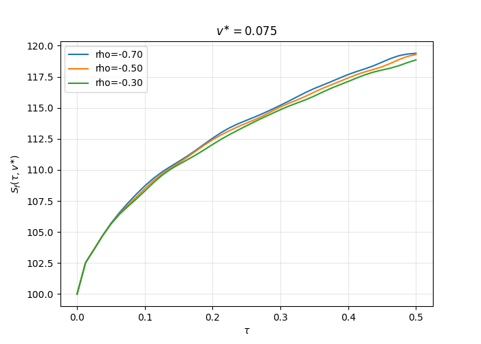
The three curves increase monotonically with \(\tau\), and for any given \(\tau\) they satisfy \[S_f(\tau,v^{*};\rho=-0.70)\;>\;S_f(\tau,v^{*};\rho=-0.50)\;>\;S_f(\tau,v^{*};\rho=-0.30). \label{eq:rho_order_boundary} \tag{44}\]
Hence, a stronger negative correlation shifts the free boundary upward.
This pattern can be interpreted through the leverage effect: a more negative \(\rho\) implies that a price decline is more likely to be accompanied by an increase in variance, thereby raising future uncertainty and the option’s continuation value. Conditional on \(v^{*}\), this reduces the relative attractiveness of locking in immediately, so the holder requires a higher underlying price \(S\) to trigger the lock-in decision, which manifests as an upward shift of the free boundary.
Keeping all other model parameters and numerical settings fixed, we compare three maturities \(T\in\{0.5,\,0.75,\,1.0\}\). Figure 2 indicates that the free boundary \(S_f(\tau,v)\) exhibits a stable and consistent structure across these maturities: it increases with the remaining time to maturity \(\tau\) and shifts upward as the variance level \(v\) increases. This behavior reflects that a longer time horizon and higher uncertainty both enhance the continuation value of retaining the option to lock in later, thereby postponing the lock-in decision and raising the optimal trigger level.
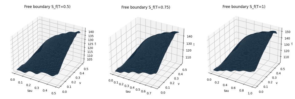
A closer comparison across maturities further shows that, as \(T\) increases, the boundary surface is lifted more noticeably in the region of larger \(\tau\), and the uplift is more pronounced at higher variance levels \(v\). This indicates that extending the maturity strengthens the continuation value associated with delaying the lock-in decision, thereby raising the opportunity cost of locking in prematurely.Consequently, a higher underlying price level \(S\) is required to trigger the lock-in decision. These findings are consistent with the financial intuition behind the maturity effect and also imply that the lock-in threshold of long maturity products is more sensitive to the prevailing volatility state.
This paper develops a numerical pricing framework for active lock-in call options within the modeling and solution paradigm of linear complementarity problems. By employing an IMEX finite difference discretization, the continuous time pricing problem is transformed into a sequence of time stepping discrete complementarity systems, which are efficiently solved using the PSOR algorithm. The resulting numerical scheme is both stable and computationally efficient. It not only provides numerical approximations of the option value function, but also lays a solid foundation for the subsequent extraction and analysis of the associated free boundary.