
This paper extends the classical logistic law (1) by introducing autonomously generated time variability in its fundamental parameters. In particular, the intrinsic growth rate \(\gamma(t)\) and the carrying capacity \(K(t)\) are allowed to evolve dynamically, following logistic modulation laws that are prescribed independently of the population state. Within this framework, population dynamics are governed by a non-autonomous logistic equation whose coefficients are themselves driven by simple yet meaningful autonomous evolutionary dynamics.
The main objectives of this work are threefold:
\(\bullet\) to investigate the effects of logistic variability in the parameters \(K(t)\) and \(\gamma(t)\) on the qualitative behavior of the population dynamics described by Eq. (1); \(\bullet\) to derive closed-form analytical solutions, expressed in terms of hypergeometric functions, and to complement these results with illustrative numerical simulations aimed at validating the analytical expressions and highlighting the resulting dynamical behavior;
\(\bullet\) to examine how the global behavior of the system can be effectively regulated by tuning a reduced set of parameters, thereby providing a parsimonious yet flexible modeling framework.
By combining analytical derivations with illustrative numerical examples, the present study aims to clarify how time-dependent coefficient dynamics, generated independently of the population variable, can be embedded in classical growth models to capture non-autonomous interactions commonly observed in real-world systems.
The analysis focuses primarily on a logistic equation with a dynamically evolving carrying capacity and is subsequently extended to account for time-dependent structures in the intrinsic growth rate \(\gamma(t)\) and carrying capacity \(K(t)\). Rather than addressing isolated special cases, the proposed framework emphasizes the general mechanisms by which parameter variability influences both transient and asymptotic regimes.
A key implication of this approach is the ability to steer the system dynamics by controlling the trajectories of \(\gamma(t)\) and \(K(t)\). This feature not only simplifies the mathematical treatment but also provides a practical tool for applications in which resource availability and population pressure co-evolve through externally prescribed or internally generated coefficient paths. In contexts such as aquaculture, wildlife management, or renewable resource exploitation, the model can inform decisions on initial population levels and intervention strategies to prevent overexploitation, excessive mortality, or inefficient resource use.
In this perspective, the extended logistic framework contributes both to the theoretical understanding of non-autonomous dynamical systems and to the development of analytically grounded models that support sustainable management practices in ecological and economic settings. The contribution of this paper is primarily theoretical. The proposed framework is designed to provide an explicit closed-form solution for a non-autonomous logistic equation with structured time-dependent coefficients. Rather than introducing new feedback mechanisms or a general modeling paradigm, the results are intended as exact benchmark solutions that can support numerical investigations and comparative analyses in more general settings where closed-form solutions are not available.
Population dynamics is a fundamental subject across disciplines including biology, genetics, demography, and epidemiology. Mathematical models play a crucial role in elucidating these dynamics, and the logistic differential equation is a primary tool for describing and analyzing population growth. Verhulst initially proposed the logistic model [1] and can be expressed as follows: \[\label{(1.1)} \dot{S}(t) = \gamma \; \!\biggl(1 – \frac{S(t)}{K}\biggr)\, S(t), \quad t\in\mathbb{R},\quad \gamma,\, K > 0. \tag{1}\]
In this context, the constant \(K>0\) is identified as the carrying capacity, and in its simplest form, it is assumed to be fixed. The positive parameter \(\gamma\) regulates the growth dynamics of the population \(S(t)\); specifically, it represents the per-capita net reproductive rate, defined as the average number of births minus deaths per individual (see [2]).
This equation, owing to its versatility, has gained considerable popularity and has been used in various bio-mathematical models to describe the temporal evolution of a species, whose numerical value at time \(t\) is denoted by \(S(t)\). The Eq. (1) was derived as an alternative to the Malthusian model, \(\dot{S}(t)=\gamma S(t)\), which, in the long term, leads to unbounded and thus physically implausible population growth. Conversely, the Verhulst model, also known as the logistic growth model or logistic, captures the self-limiting boundary encountered by population expansion. As detailed in [2], the population exhibits exponential growth when the population size is minimal; however, for larger values, factors such as crowding, food scarcity, and environmental influences become significant.
In applied mathematics, the logistic model has been extensively validated using empirical data from various biological systems. Initial research by G.F. Gause, N.P. Smaragdova, and A.A. Witt in the 1930s confirmed its ability to accurately depict predator–prey interactions [3]. Pearl and Reed effectively employed it to model the growth of the United States population [4]. More broadly, mathematical biology remains one of the primary disciplines that use the logistic equation, as evidenced by comprehensive analyses in Edelstein‑Keshet [5] and Murray [6].
Eq. (1) has also been widely used in bio-economic models of sustainable resource management, as exemplified in Clark’s monograph on renewable resources [7] and in ecological harvesting strategies, as discussed by Kot [8]. In economic applications, the function \(S(t)\) often represents the number of prospective buyers for a product, as in the research of Alliney [9] and Ritelli, Barbiroli, and Fabbri [10]. An influential example is the Fisher–Pry model of technological substitution [11], in which \(S(t)\) denotes the market share of an emerging technology. Initially, adoption is driven by positive feedback, so that each new user stimulates further adoption; however, as the pool of remaining potential adopters diminishes, the growth rate decelerates and ultimately reaches a plateau. This dynamic, characterized by autocatalytic dissemination and saturation, yields the classic sigmoid diffusion curve observed in numerous innovation diffusion phenomena.
Eq. (1) is a differential equation of the form \[\dot{S}(t)=g(S(t))S(t),\] where \(g:[0,\infty )\rightarrow \Bbb{R}\) is a differentiable function with \(g^{\prime }(S)\leq 0\) and such that \(g(0)=a>0\); furthermore we assume that there exists \(K_{0}>0\) such that \(g(K_{0})=0.\)
This is the concept of ‘‘dynamic’’ introduced by Freedman [12] in his research on antiparasitic conflict, specifically through the engagement of a natural enemy of the parasites within biological agriculture. It is also discussed in [2]. Subsequently, this concept has been proposed within economic models as well (see [10]), where the core idea is that \(S(t)\) represents the demand for a good at time \(t\), with its dynamics governed by the logistic differential equation. In such cases, this can be correlated with other scalar differential equations that model the dynamics of the goods’ producers.
Nonetheless, there is a long-standing interest in generalizing the classical logistic Eq. (1), motivated not only by theoretical considerations but also by the need for more flexible and realistic modeling frameworks. In this direction, a seminal contribution is due to Nkashama [13], who studied the non-autonomous logistic equation \[\label{2.2} \dot{u}(t)=u(t)\big[ A(t)-B(t)u(t)\big],\quad t\in \mathbb{R}. \tag{2}\]
Under strong assumptions on the coefficient functions, including continuity, strict positivity, boundedness away from zero, and almost-periodicity of \(A,B:\mathbb{R}\to\mathbb{R}\), Nkashama established fundamental results concerning the existence, uniqueness, positivity, and global attractor structure of solutions. More precisely, assuming the uniform bounds \[\label{ineq:ineq1} 0<\alpha_0 \leq A(t)\leq \alpha_1,\quad 0<\beta_0 \leq B(t)\leq \beta_1,\quad t\in\mathbb{R}. \tag{3}\]
Nkashama proved the existence of a unique positive bounded solution acting as a global forward attractor, together with a backward exponential stability of the zero solution. These results provide an important historical benchmark in the theory of non-autonomous logistic equations.
The primary objective of this paper is to explore and extend the classical logistic law (1), allowing its key parameters, the intrinsic growth rate \(\gamma\) and the carrying capacity \(K\), to vary over time. In particular, we introduce logistic–type feedback in which \(\gamma\) and/or \(K\) evolve according to their own logistic dynamics.
Allowing \(\gamma\) and \(K\) to depend on time accommodates realistic scenarios in which reproduction rates and resource limitations vary, due to factors such as climate cycles, harvesting policies, or technological and ecological developments. By treating these parameters as either externally prescribed or governed endogenously by supplementary logistic laws, we establish a versatile framework that bridges the divide between basic autonomous models and more plausible non-autonomous systems.
Our analysis proceeds in two main stages:
(1) we model (1) by considering \(\gamma\) and/or \(K\) themselves to evolve according to logistic dynamics, thereby extending the classical formulation through nested feedback structures.
(2) we provide symbolic examples and numerical simulations to illustrate how the logistic variability of parameters affects transient and asymptotic behaviour of the system. These examples highlight both the robustness of the model and its applicability in concrete management contexts.
A principal motivation for this research is the potential to regulate the system by adjusting only two parameters. This economical configuration not only facilitates mathematical analysis but also provides practical tools for developing sustainable strategies. By selecting appropriate initial conditions and parameter trajectories, resource allocation within the system can be optimized, thereby reducing inefficiencies and waste. For instance, in fisheries and aquaculture, our framework may inform the selection of initial stocking levels to prevent overpopulation, mortality peaks, or underutilization of the available environment. Similar interpretations apply to ecological reserves or the management of renewable resources, where logistic feedback on environmental support can indicate either degradation or recovery of natural habitats.
By integrating rigorous analysis with illustrative case studies, this work demonstrates how the logistic law can be enhanced to more accurately describe systems subject to dynamic environmental constraints and reproductive potential. The resulting framework advances both theoretical understanding of non-autonomous differential equations and practical applications in population management, economic planning, and sustainability policies.
Before proceeding, we summarize the notation and the variables used throughout the paper. The main quantity of interest is the population size \(S(t)\), whose dynamics are governed by a non-autonomous logistic equation with time-dependent coefficients. Specifically,
\(\bullet\) \(S(t)\) denotes the population size at time \(t\);
\(\bullet\) \(S_0\) is the initial population size, i.e. \(S(0)=S_0>0\);
\(\bullet\) \(\gamma(t)>0\) is the intrinsic growth rate, evolving according to a prescribed logistic law, and \(\gamma_0=\gamma(0)\) denotes its initial value, while \(\bar{\gamma}\) represents the constant intrinsic growth rate;
\(\bullet\) \(a\) and \(b\) are the coefficients of the logistic law governing the evolution of \(\gamma(t)\);
\(\bullet\) \(K(t)>0\) is the carrying capacity, evolving according to a prescribed logistic law;
\(\bullet\) \(\alpha\) and \(\beta\) are the coefficients of the logistic law governing the evolution of \(K(t)\);
\(\bullet\) \(K(0)=K_0\) denotes the initial value of the carrying capacity, while \(\bar{K}\) represents the constant carrying capacity.
Throughout the paper, the time domain is assumed to be \(t\ge 0\), which is the standard setting for population models with prescribed initial conditions.
In epidemiological and ecological applications, permitting the parameters of the logistic model, notably the carrying capacity \(K\) and the growth rate \(\gamma\), to vary over time enables a more comprehensive and realistic representation of real-world dynamics. For example, in infectious disease modeling, a time-dependent \(K(t)\) effectively captures the impacts of public health interventions such as social distancing, mask mandates, vaccination programs, and the administration of antiviral or monoclonal antibody therapies, all of which serve to decrease the effective susceptible population and consequently limit the maximum extent of the epidemic.
Beyond epidemiology, variable coefficients hold equal significance within pure biological contexts. In population ecology, a time-dependent carrying capacity aptly characterizes seasonal fluctuations in resource availability, including food supply, habitat space, or water levels, which subsequently influence boom-and-bust cycles in species populations. Variable growth rates can effectively model temperature-dependent metabolic rates in ectotherms or reproductive suppression caused by stress under adverse conditions.
Mathematically, these extensions of (1) take the form of \[\label{3.1} \begin{cases} \dot{S}(t) \;=\; \gamma(t)\,\Bigl(1 – \frac{S(t)}{K(t)}\Bigr)\;S(t),\\[6pt] S(0) = S_{0} > 0, \end{cases} \tag{4}\] where \(\gamma(t)\) and \(K(t)\) are governed by additional differential equations within a coupled system, such as a logistic differential equation. Foundational contributions in this area include Nkashama’s non-autonomous almost-periodic logistic model [13], Meyer’s seasonal resource-driven population model [14], and related contributions in [15]. These frameworks facilitate the analysis of the interactions between external forcing and internal feedback mechanisms in shaping transient dynamics, stability features, and long-term persistence. Such insights are indispensable for both epidemic management and the conservation of biological populations.
Eq. (4) can be integrated, and in particular, by changing the variable \(S = u^{-1}\), it is a Bernoulli equation. The solution, which can be obtained using standard undergraduate-level techniques, is: \[\label{3.2} S(t)=\frac{ \exp \left(\int _0^t\gamma (\tau){ d}\tau\right)}{\frac{1}{S_0}+ \int _0^t\frac{\gamma (\tau)}{K(\tau)}\exp \left(\int _0^{\tau}\gamma (\xi )\,{ d}\xi \right)\, { d}\tau}. \tag{5}\]
In light of the represention depicted in (2), we note that \[A(t) = \gamma(t), \quad B(t) = \frac{\gamma(t)}{K(t)}.\]
The initial section of the contribution seeks to identify potentially explicit solutions to (4), permitting variability of \(\gamma(t)\) and \(K(t)\) that is governed by a logistic differential equation in both cases. We will examine the two scenarios separately, i.e., taking \(K(t) = {\bar{K}}\) as fixed, while \(\gamma(t)\) is variable, and vice versa. Subsequently, we will also present the results in which both parameters vary in a logistic manner.
Assuming to work with the expression of the logistic equation in (4), we let \(\gamma(t)\) and \(K(t)\), to follow these dynamics: \[\label{3.1.1} \begin{cases} \dot{\gamma}(t) \;=\; a\,\gamma(t)-b\,\gamma(t)^2,\\[6pt] \gamma(0) = \gamma_{0} > 0, \end{cases} \tag{6}\] and \[\label{3.1.2} \begin{cases} \dot{K}(t) \;=\; \alpha\,K(t)-\beta\,K(t)^2,\\[6pt] K(0) = K_{0} > 0. \end{cases} \tag{7}\]
The solution to (6) and (7) are respectively \[\label{gammaKappa} \gamma(t) = \frac{a}{b+\left( \frac{a}{\gamma_{0}} – b\right) e^{-a t}} \quad \text{and} \quad K(t) = \frac{\alpha}{\beta+\left( \frac{\alpha}{K_{0}} – \beta\right) e^{-\alpha t}}, \tag{8}\] as a logistic law of the form drives them (2), with parameters \(a,\, b,\, \alpha,\, \beta > 0.\)
Consider the Eq. (4) assuming \(\gamma(t)\) is defined in (8) and \(K(0) = {\bar{K}}\), so we are implicitly working with a fixed carrying capacity while a variable net reproduction rate of the population. According to these assumptions, (4) becomes \[\label{K0} \begin{cases} \dot{S}(t) \;=\; \gamma(t)\,\Bigl(1 – \frac{S(t)}{{\bar{K}}}\Bigr)\;S(t),\\[6pt] S(0) = S_{0} > 0. \end{cases} \tag{9}\]
From (5), we have that the solution to (9), after straightforward but elementary computations, is \[%\label{3.8} S(t)= \frac{a^{-\frac{1}{b}} \left(b \gamma_0 \left(e^{a t}-1\right)+a\right)^{\frac{1}{b}}}{\frac{1}{S_0}+ \frac{1}{{\bar{K}}}\left(a^{-\frac{1}{b}} \left(b \gamma_0 \left(e^{a t}-1\right)+a\right)^{\frac{1}{b}}-1 \right) }.\]
Conversely, similar results can be derived by incorporating into the Eq. (4) a variable term representing the carrying capacity, denoted as \(K(t)\), which is governed by a logistic growth law. Meanwhile, the net reproduction rate \(\gamma(t)\) remains constant at \({\bar{\gamma}}\) for all \(t\). Consequently, this model examines the impact of a time-dependent carrying capacity, adhering to a logistic law, while maintaining the net reproduction rate as constant. Therefore, from (5) we get \[\label{gammafixed} S(t) =\frac{e^{{\bar{\gamma}}}} {\displaystyle\frac{1}{S_0} +{\bar{\gamma}}\int_{0}^{t}\frac{e^{{\bar{\gamma}}\tau}}{K(\tau)}\,{ d}\tau}\,. \tag{10}\]
Integrating the denominator term by term, one finds \[\int_{0}^{t}\frac{e^{{\bar{\gamma}}\tau}}{K(\tau)}\,{ d}\tau =\frac{\beta\bigl(e^{{\bar{\gamma}} t}-1\bigr)}{\alpha} +\frac{{\bar{\gamma}}\,\beta\bigl(e^{({\bar{\gamma}}-\alpha)t}-1\bigr)}{\alpha(\alpha-{\bar{\gamma}})} +\frac{{\bar{\gamma}}\bigl(1-e^{({\bar{\gamma}}-\alpha)t}\bigr)}{\alpha K_0-{\bar{\gamma}}K_0}\,,\] thus (10) becomes \[S(t) =\frac{e^{{\bar{\gamma}} t}} {\displaystyle \frac{1}{S_0} +\frac{\alpha{\bar{\gamma}} +\alpha\,\beta\,K_0\,e^{{\bar{\gamma}} t} -{\bar{\gamma}}(\alpha-\beta\,K_0)e^{({\bar{\gamma}}-\alpha)t} -\alpha\,\beta\,K_0 -{\bar{\gamma}}\,\beta\,K_0\,e^{{\bar{\gamma}} t}} {\alpha\,K_0\,(\alpha-{\bar{\gamma}})} }\,.\]
Finally, it is possible to derive analogous results by incorporating, as a variable component in (4), the carrying capacity \(K(t)\) governed by a logistic evolution law, and by allowing the net reproduction rate \(\gamma(t)\) to vary as described in (8). Thus, this model investigates the effects of a time-dependent carrying capacity following a logistic trajectory, in conjunction with a fluctuating net reproduction rate, thereby enhancing the model’s complexity and robustness.
Accordingly, from (5) and calling with \(I(t)\) the integral of \(\gamma (\tau)\) in \([ 0, t]\): \[\label{It} I(t) = \int _0^t\gamma (\tau) { d}\tau = \int _0^t \frac{a}{b+\left( \frac{a}{\gamma_{0}} – b\right) e^{-a \tau}} \text{ d }\tau = \frac{\ln \left(b \gamma_0 \left(e^{a t}-1\right)+a\right)-\ln a}{b}, \tag{11}\] we find the solution \[\label{solGen} S(t) =\frac{e^{I(t)}} {\displaystyle \frac{1}{S_0} +\int_{0}^{t}\frac{\gamma(\tau)}{K(\tau)}\,e^{I(\tau)}\,\text{ d }\tau }\,. \tag{12}\]
This implies that we must evaluate the following integral:
\[%\label{NtOr} N(t) = \int_{0}^{t}\frac{\gamma(\tau)}{K(\tau)}\,e^{I(\tau)}\,\text{ d }\tau,\] and, after some standard computations, we get \[N(t)=\int_{0}^{t} \frac{a^{1-\frac{1}{b}} \, \left(b \gamma_0 \left(e^{a \tau }-1\right)+a\right)^{\frac{1}{b}}\,\left(e^{-\alpha \tau } \left(\frac{\alpha}{K_0}-\beta\right)+\beta\right)}{\alpha \, \left(e^{-a \tau } \left(\frac{a}{\gamma_0}-b\right)+b\right)} \,\text{ d }\tau\,.\]
We perform the change of variable \(x=e^{a\tau}\), so that we obtain, after some simplifications, \[\label{Nt} N(t) =\frac{\gamma_0 a^{-\frac{1}{b}}}{\alpha K_0} \int_{1}^{e^{at}} (a+b\gamma_0 (x-1))^{\frac{1}{b}-1} \left(x^{-\frac{\alpha}{a}} (\alpha-\beta K_0)+\beta K_0\right)\, \text{ d } x, \tag{13}\] that can be split into \[\frac{\gamma_0 a^{-\frac{1}{b}}}{\alpha K_0}\left( \int_{1}^{e^{at}} \beta K_0 (a+b \gamma_0 (x-1))^{\frac{1}{b}-1} \, \text{ d }x + \int_{1}^{e^{at}} x^{-\frac{\alpha}{a}} (\alpha-\beta K_0) (a+b \gamma_0(x-1))^{\frac{1}{b}-1} \, \text{ d }x \right).\]
The first integral is elementary, indeed, letting \(s = a+b \gamma_0 (x-1)\), we get \[\label{intt1} \beta\, K_0 \int_{a}^{b \gamma_0\left(e^{a t}-1\right)+a} s^{\frac{1}{b}-1} \, \text{d}s = \frac{\beta K_0 \left(\left(b \gamma_0 \left(e^{a t}-1\right)+a\right)^{\frac{1}{b}}-a^{\frac{1}{b}}\right)}{\gamma_0}. \tag{14}\]
On the other hand, to compute the second integral, we make use of a strategy already presented in [15], that deals with splitting the domain of integration into two sub-integrals and using a result presented in [16].
So, we have that \[\label{intt2} (\alpha-\beta K_0)\, \int_{1}^{e^{at}} x^{-\frac{\alpha}{a}} \left(a+b \gamma_0\,(x-1)\right)^{\frac{1}{b}-1} \, \text{d}x = (\alpha-\beta K_0)\, \left( M(t) – M(0) \right) , \tag{15}\] where \[\label{M-t} M(t) = \int_{0}^{e^{at}} x^{-\frac{\alpha}{a}} \left(a+b \gamma_0\,(x-1)\right)^{\frac{1}{b}-1} \, \text{d}x. \tag{16}\]
Note that
\(\bullet\) \(a + b \gamma_0 ( x- 1) = a-b \gamma_0 +b \gamma_0 x\)
\(\bullet\) \(\left( a-b \gamma_0 +b \gamma_0 x\right)^{\frac{1}{b}-1} = b \gamma_0^{\frac{1}{b}-1}\left(\frac{a-b \gamma_0}{b \gamma_0} + x\right)^{\frac{1}{b}-1}\)
which, assuming \(a > b\gamma_0\) and \(\ 1-\frac{\alpha}{a}> 0\), allows us to use the entry 3.197.8 page 317 of [16].
Indeed, we have that \[\label{M-t2} M(t)= \frac{a \left(\frac{a-b \gamma_0}{b \gamma_0}\right)^{\frac{1}{b}-1} e^{t (a-\alpha)} b \gamma_0^{\frac{1}{b}-1}}{a-\alpha}\, _2F_1 \left( 1-\frac{1}{b},\,1-\frac{\alpha}{a}, \,2-\frac{\alpha}{a}, \, -\frac{b e^{a t} \gamma_0}{a-b \gamma_0} \right),\] and similarly \[M(0) = \frac{a \left(\frac{a-b \gamma_0}{b \gamma_0}\right)^{\frac{1}{b}-1}b \gamma_0^{\frac{1}{b}-1}}{a-\alpha} \, _2F_1 \left( 1-\frac{1}{b},\,1-\frac{\alpha}{a}, \,2-\frac{\alpha}{a}, \, -\frac{b \gamma_0}{a-b \gamma_0} \right).\]
Note that a condition for the convergence of the integral, according to the entry 3.197.8 page 317 of [16], we need that \(\alpha<a\) and \(a > b\gamma_0\).
The computation of the integral (16) relate to Euler’s integral representation of the Gauss Hypergeometric Function \(_2F_1\) (see [17– 19]): \[\label{irt} \begin{split} _2F_1\left(l, \, m, \, q ,\, z \right) & =\sum_{n=0}^\infty \frac{(l)_n (m)_n}{(q)_n}\frac{z^n}{n!} \\ & =\frac{\Gamma(q)}{\Gamma(q-m)\,\Gamma(m)}\int_0^1 t^{m-1}(1-t)^{q-m-1}(1-zt)^{-l}\text{ d }t, \end{split} \tag{17}\] where \((.)_{n}\) is a Pochhammer symbol. The series is convergent for any \(l,\;m,\;q\) if \(|z|<1\), and for \(Re\,(l+m-q)<0\) if \(|z|=1\). For the integral representation is required \(Re\,(q)>Re\,(m)>0\). Here \(\Gamma(z)\) denotes the Gamma Function. A quick overview of Gauss Hypergeometric Function can be found in [20]. The steps to obtain (15) via (17) are the same as those presented in [21], and are based on the decomposition of the integral as the difference between the integral from \(0\) to the upper limit and the integral from \(0\) to \(1\), followed by the normalization of the first integral in order to exploit the integral representation (17) theorem of the Hypergeometric function.
Finally, combining together (14) and (15), we have that (13) is \[N(t)= \frac{\gamma_0 a^{-\frac{1}{b}} (\alpha-\beta K_0)(M(t)-M(0)) +\beta K_0 \left(a^{-\frac{1}{b}} \left(b \gamma_0 \left(e^{a t}-1\right)+a\right)^{\frac{1}{b}}-1\right)}{\alpha K_0},\] and to get (12), we recall (11), obtaining \[\label{solFin} S(t) = \frac{e^{I(t)}}{\frac{1}{S_0}+ N(t)}. \tag{18}\]
The integral in Eq. (16) cannot be expressed in terms of elementary functions. For this reason, hypergeometric functions provide a natural and effective analytical framework to represent the solution of the differential equation in closed form. This exact representation is not pursued for its own sake, but rather because it offers a rigorous analytical benchmark that can support, validate, and corroborate numerical implementations, especially in regimes where purely numerical approaches may obscure the structural dependence on the model parameters.
Table 1 reports the relative error
associated with the solution provided by Eq. (18),
computed by comparing the numerical approximation with the corresponding
analytical expression. The numerical solution used for comparison was
computed by means of the NDSolve solver implemented in
Mathematica. The error is evaluated for increasing values of
the final time \(T\), using the
following set of parameters: \[a=\frac{1}{2},
\quad b=\frac{1}{4},
\quad \alpha=\frac{1}{8},
\quad \beta=\frac{1}{9},
\quad \gamma_0=\frac{1}{20},
\quad K_0=\frac{1}{2},
\quad S_0=8.\]
| Final time \(T\) | \(\displaystyle {{\mathrm{error}}(T) = \frac{ \max_{t\in[0,T]} \left| S_{\mathrm{num}}(t)-S_{\mathrm{ana}}(t) \right| }{ \max_{t\in[0,T]} \left| S_{\mathrm{ana}}(t) \right| }}\) |
|---|---|
| \(30\) | \(1.61859\times 10^{-7}\) |
| \(31\) | \(1.61859\times 10^{-7}\) |
| \(32\) | \(1.61859\times 10^{-7}\) |
| \(33\) | \(1.61859\times 10^{-7}\) |
| \(34\) | \(1.61859\times 10^{-7}\) |
| \(35\) | \(1.61859\times 10^{-7}\) |
| \(36\) | \(1.61859\times 10^{-7}\) |
| \(37\) | \(1.61859\times 10^{-7}\) |
| \(38\) | \(1.61859\times 10^{-7}\) |
| \(39\) | \(1.61859\times 10^{-7}\) |
| \(40\) | \(1.61859\times 10^{-7}\) |
The results reported in Table 1 show that the relative error remains uniformly bounded and stable as the final time \(T\) increases, providing further evidence of the accuracy and consistency of the analytical solution (18).
This section presents several simulations concerning the model delineated in (12), which considers the scenario where both coefficients of Eq. (4) exhibit logistic variation. Firstly, it is essential to note that (12), to ensure the convergence of the integral, needs that \(\alpha<a\) and \(a > b\gamma_0\). A first consequence of this binding condition on the parameters is related to the behaviour of the \(\gamma(t)\). Indeed, \[\dot{\gamma}(t) = \frac{a^2 e^{-a t} \left(\frac{a}{\gamma _0}-b\right)}{\left(e^{-a t} \left(\frac{a}{\gamma _0}-b\right)+b\right)^2} > 0 ,\] which implies that \(\gamma(t)\) is strictly increasing since we assume that \(a > b\gamma_0\). In practical terms, this indicates that the net population growth rate remains consistently positive and does not alter its sign, thereby ensuring that it maintains biological relevance as a positive value.
Moreover, by (4), we have \[\begin{aligned} \ddot{S}(t) & = \frac{S(t)}{K(t)^2} \left[\gamma (t) \left(S(t) \; \dot{K}(t)\; +\gamma (t) (K(t)-S(t)) (K(t)-2 S(t))\right) + K(t) \Big(K(t)-S(t)\Big) \dot{\gamma}(t)\;^{}_{} \right], \end{aligned}\] where the last equation comes from the substitution of the right hand side of (4). We notice that \(\dot{S}(t) = 0\) if
\(\bullet\) \(S(t) = 0\);
\(\bullet\) \(S(t) = K(t)\).
Considering the non-trivial solution \(S(t) = K(t)\), we get that \[\label{derivata2} \ddot{S}(t) = \gamma(t) \, \dot{K}(t). \tag{19}\]
Since \(\gamma(t) > 0\) according to (8) and due to the fact that \(a > b\gamma_0\), the sign of Eq. (19) depends only on \(\dot{K}(t)\), i.e., \[\label{derivataKappa} \dot{K}(t) = \frac{\alpha ^2 e^{- \alpha t} \left(\frac{\alpha }{K_0}-\beta \right)}{\left(\beta +e^{- \alpha t} \left(\frac{\alpha }{K_0}-\beta \right)\right)^2}. \tag{20}\]
All the parameters of (20) are positive and therefore the sign of (20) depends only on the quantity \(\frac{\alpha }{K_0}-\beta\). Therefore the sign of (19) ultimately depends on the the quantity \(\frac{\alpha }{K_0}-\beta\), and in particular \[\label{derivata2-param} \ddot{S}(t) < 0 \quad \textrm{if} \; \alpha < K_0 \, \beta, \qquad \ddot{S}(t) > 0 \quad \textrm{if} \; \alpha > K_0 \, \beta. \tag{21}\]
Ultimately, the scenario associated with \(\ddot{S}(t) < 0\) pertains to the existence of a local (or global) maximum in the solution of (12), while \(\ddot{S}(t) > 0\) indicates the existence of a local (or global) minimum for the solution of (12). In the remainder of this section, we will present several simulations that illustrate the characteristics of the general solution that have just been highlighted.
Finally, it is interesting to see which is the long-term equilibrium of (12), i.e., applying the de l’Hôpital rule, assuming that \(a, b, \gamma, K_0, S_0 >0\) and \(\alpha<a,\; a>b\gamma_0\), we obtain \[\label{limite} \lim_{t\to \infty} S(t) = \lim_{t\to \infty} \frac{e^{I(t)}}{\frac{1}{S_0}+ N(t)} = \frac{\alpha}{\beta}. \tag{22}\]
Indeed, notice that \[\lim_{t\to \infty} e^{I(t)} = \lim_{t\to \infty} a^{-\frac{1}{b}}(b\gamma_0)^{\frac{1}{b}} e^{\frac{a}{b}t},\] since as \(t \to +\infty\), \[a+b(-1+e^{at})\gamma_0 \;\sim\; b\gamma_0 e^{at} \quad \Longrightarrow \quad \big(a+b(-1+e^{at})\gamma_0\big)^{\frac{1}{b}} \;\sim\; (b\gamma_0)^{\frac{1}{b}} e^{\frac{a}{b}t}.\]
On the other hand, the denominator is dominated by \[\frac{1}{K_0\alpha}\,a^{-\frac{1}{b}}\gamma_0 \left(K_0\beta\, b^{\frac{1}{b}}\gamma_0^{\frac{1}{b}-1} e^{\frac{a}{b}t}\right) \;=\;\frac{\beta}{\alpha}\,a^{-\frac{1}{b}} b^{\frac{1}{b}}\gamma_0^{\frac{1}{b}} e^{\frac{a}{b}t}.\]
Therefore, \[\lim_{t\to \infty} S(t) = \lim_{t\to \infty} \frac{a^{-\frac{1}{b}}(b\gamma_0)^{\frac{1}{b}} e^{\frac{a}{b}t}}{\frac{\beta}{\alpha}\,a^{-\frac{1}{b}} (b \gamma_0 )^{\frac{1}{b}} e^{\frac{a}{b}t}} = \frac{\alpha}{\beta}.\]
For clarity, we explicitly list below the assumptions on the model parameters used throughout the analytical derivation. These conditions serve two distinct purposes: biological plausibility and analytic convergence.
\(\bullet\) Biological plausibility. We assume \[a>0,\quad b>0,\quad \gamma_0>0,\quad K_0>0,\quad S_0>0,\] which ensure positivity of the intrinsic growth rate, carrying capacity, and population size. These assumptions are standard in population dynamics models and exclude biologically meaningless negative quantities.
\(\bullet\) Analytic convergence. The conditions \[\alpha<a,\qquad a>b\gamma_0,\] are required to guarantee the convergence of the integral representations used in the hypergeometric reduction. Under these assumptions, the relevant integrals admit closed forms in terms of hypergeometric functions. If these conditions are not satisfied, the integral representations cannot be employed and the solution must be obtained through numerical integration.
We further observe that one of the analytic conditions, namely \(a>b\gamma_0\), also implies that the intrinsic growth rate \(\gamma(t)\) is strictly increasing. This feature reinforces the modeling framework, as it corresponds to a scenario in which the population’s intrinsic growth potential improves over time, consistently with the assumed evolutionary setting.
Figure 1 illustrates the behavior of the solutions \(\gamma(t)\) and \(K(t)\) in (8), considering two contrasting evolutions for the coefficients. Indeed, \(K(t)\) is decreasing, reaching its asymptote, bearing in mind that \(\gamma(t)\ \) is strictly increasing.
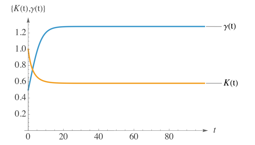
Figure 1 depicts \(\gamma(t)\) increasing with a classic S-shaped curve from an initial low value towards a steady plateau. This illustrates a net reproduction rate that increases over time, potentially as individuals reach maturity or breeding conditions improve, before stabilizing at its maximal sustainable level.
Conversely, Figure 1 demonstrates that \(K(t)\) decreases rapidly from an initially elevated capacity towards a lower asymptote. This signifies an environment or resource base that initially seems abundant but diminishes over time as a result of overexploitation, contamination, or habitat destruction, eventually stabilizing at a diminished long-term carrying capacity.
Together, these complementary trends exemplify a system in which reproductive potential augments despite diminishing environmental support, culminating in a period during which increased breeding success partially offsets habitat decline, ultimately attaining a steady state wherein both rates and capacities stabilize.
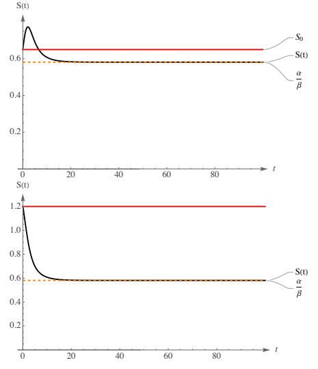
The initial image in Figure 2 illustrates a sudden increase in the (12). Specifically, within this context, it is observed that \(S_0 < K_0\); the system is compelled to reach the carrying capacity during its initial phase, for \(t\) close to 0. Evidently, since the carrying capacity \(K(t)\) also varies logistically, the system does not attain the value of \(K_0\). However, during its initial stage, a significant increase in the population \(S(t)\) can be observed. In other words, the population size at time \(t=0\) is less than \(K_0\), thus compelling the solution to increase, driven by a favorable carrying capacity. According to (21), it is established that \(\alpha = 0.25 < \beta K_0 = 0.43\), thereby confirming that \(\ddot{S}(t) < 0\), which signifies the presence of either a local or global maximum within the population dynamics. It is evident that subsequent to a phase of significant growth, a peak value is reached, after which the population commences to decline. The initial analysis provided at the outset of this section serves as a crucial tool for scrutinizing the system’s development and for resource management. In the context of fish aquaculture, for instance, it is unfavorable from both an economic and sustainability perspective to experience a swift increase in population size that is then followed by a decline. Furthermore, from (22), it is understood that the system, as time approaches infinity, attains its asymptotic value represented by \(\frac{\alpha}{\beta}\). The intriguing aspect is that the long-term equilibrium of \(S(t)\) is entirely dependent on the parameters of the logistic carrying capacity; therefore, as we have the ability to control the initial number of individuals \(S_0\), by simply managing the ratio \(\frac{\alpha}{\beta}\), we are able to avoid waste of resources. Indeed, it is generally undesirable for \(S_0 > \frac{\alpha}{\beta}\); rather, the contrary is preferable, considering both economic and sustainability viewpoints.
Conversely, the second image in Figure 2 illustrates a scenario where there is an immediate, rapid decline in the population towards its asymptote \(\frac{\alpha}{\beta}\). This phenomenon reflects the choice of the initial condition \(S_0 > K_0\). The system does not encounter pressure to increase its population; rather, it demonstrates immediate saturation within population dynamics, characterized by a carrying capacity inadequate for ensuring the survival of all individuals. Cœteris paribus, alterations in the initial conditions influence the evolution of the system; in this instance, both conditions satisfy that \(S_0 >K_0\) and \(S_0 >\frac{\alpha}{\beta}\). From an applied perspective, this situation results in resource depletion, which is undesirable both economically and from a sustainability standpoint. Furthermore, since \(\ddot{S}(t) < 0\), the global maximum is attained at \(t = 0\), thereby indicating that a decline in the population must necessarily be observed.
Finally, it is noteworthy that these two situations share a common element: the decreasing carrying capacity. Indeed, as depicted in Figure 1, \(K(t)\) diminishes from an initial value of \(K_0\) to its asymptote at \(\frac{\alpha}{\beta}\). It is observed that in both simulations, the long-term population decreases relative to the initial conditions, attributable to the decline of \(K(t)\), indicating that the model is designed to be responsive to these dynamics. Specifically, the progression of \(K(t)\) may be regarded as either exogenous or endogenous; however, in general, if control over it is feasible, then the entire system’s evolution can be effectively managed.
Figure 3 demonstrates that both \(\gamma(t)\) and \(K(t)\) display the conventional S-shaped curve, indicative of logistic-type growth. The net reproduction rate \(\gamma(t)\) commences at a relatively low initial value, increases swiftly as the population matures or as conditions improve, and subsequently stabilizes near its asymptote, represented by the ratio \(\frac{a}{b}\). Similarly, the carrying capacity \(K(t)\), with an initial condition of \(K_0 = 1\), commences at a modest baseline, undergoes a significant increase as resources or habitat recover, and asymptotically approaches its carrying limit, expressed as \(\frac {\alpha}{\beta}\). The steep ascent of each curve signifies a phase of rapid enhancement, whereas the eventual plateau indicates the system’s attainment of its long-term sustainable rates and capacities.
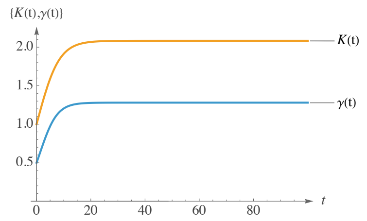
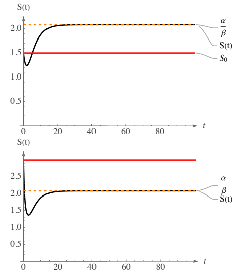
Collectively, these mutually reinforcing trends delineate a system wherein both reproductive capacity and environmental support enhance progressively over time. The population not only reproduces more effectively but also benefits from increasing resources and available space, culminating in an extended phase of accelerated growth. Ultimately, the system attains a higher equilibrium point, where amplified rates and expanded capacities are harmonized, establishing a new steady state. Nevertheless, to assess whether the system can achieve a more optimal equilibrium concerning population growth, it is essential to examine the relationship between the initial condition \(S_0\) and the long-term equilibrium \(\frac{\alpha}{\beta}\). Indeed, the curve \(S(t)\) in the initial image of Figure 4 depicts an initial sharp decline in (12).
In particular, within this context, we observe that \(S_0>K_0\), indicating that at its initial phase, when \(t \approx 0\), there exists a pressure exerted on the system to attain the carrying capacity \(K_0\). Given that \(K(t)\) also varies logistically, the system does not exactly achieve the value of \(K_0\); instead, there is a decrease in population attributable to a less favorable environment. In other words, the population size at time \(t=0\) exceeds \(K_0\), indicating that the solution is compelled to decrease due to a less favorable carrying capacity. By (21), we have that \(\alpha = 0.25 > \beta K_0 = 0.12\). This feature implies that \(\ddot{S}(t) > 0\), so that there is a local or global minimum in the population dynamics. Indeed, as we can observe, after the period of strong decrement, it is clear that there is a minimum value after which the population starts to rise; in particular, \(S(t)\) rises to reach its asymptote, i.e., (22), that is higher than \(S_0\); this simulation reflects that the system is able to reach a higher level of equilibrium, exploiting the fact that this one is fully derived by the parameters of \(K(t)\).
On the other hand, the second image in Figure 4 displays a situation in which we immediately observe a rapide decline of the population, that goes even lower than its asymptote \(\frac{\alpha}{\beta}\); Indeed, the initial condition is \(S_0 > \frac{\alpha}{\beta} > K_0\). The system does not feel any pressure to increase the number of individuals, since the initial population is above the carrying capacity. There is an immediate saturation in the population dynamics, characterized by a carrying capacity insufficient to ensure the survival of all individuals. Alterations to the initial conditions influence the evolution of the system, resulting in resource depletion, which is undesirable both economically and from a sustainability perspective. Following the attainment of its global minimum, the population subsequently increases, rapidly reaching a long-term equilibrium.
It is noteworthy that, although these two circumstances exemplify an increasing carrying capacity, they lead to two distinct systemic states. Indeed, as we see from Figure (3), \(K(t)\) increases from an initial value of \(K_0\), to its asymptote \(\frac{\alpha}{\beta}\). However, two simulations in Figure 4, displays two different states of the system: in the first, driven by a lower initial condition \(S_0\), the population increases with respect to the initial condition in the long term; in the second case, instead, despite \(K(t)\) is increasing, the initial condition is higher than the asymptote \(\frac{\alpha}{\beta}\), leading to a lower long-term equilibrium.
The parameter sets used in Figures 1–4 are summarized in Table 2.
| Figure | \(a\) | \(b\) | \(\gamma_0\) | \(\alpha\) | \(\beta\) | \(K_0\) | \(S_0\) |
|---|---|---|---|---|---|---|---|
| Fig. 1 | 0.32 | 0.25 | 0.5 | 0.25 | 0.43 | 1 | |
| Fig. 2 (above) | 0.32 | 0.25 | 0.5 | 0.25 | 0.43 | 1 | 0.65 |
| Fig. 2 (below) | 0.32 | 0.25 | 0.5 | 0.25 | 0.43 | 1 | 1.2 |
| Fig. 3 | 0.32 | 0.25 | 0.5 | 0.25 | 0.12 | 1 | |
| Fig. (4) (above) | 0.32 | 0.25 | 0.5 | 0.25 | 0.12 | 1 | 1.5 |
| Fig. (4) (below) | 0.32 | 0.25 | 0.5 | 0.25 | 0.12 | 1 | 3 |
The results and simulations presented in this work underscore the model’s primary characteristic, in which both coefficients of the logistic equation undergo autonomous logistic evolution prescribed independently of the population dynamics. Based on the analytical findings, we determined the conditions that guarantee the monotonicity of \(\gamma(t)\) and the asymptotic behavior of \(K(t).\) Furthermore, we clarified how the sign of the second derivative \(\ddot{S}(t)\) is influenced by the relationships among the parameters \(\alpha\), \(\beta\), and \(K_0\).
In particular, we demonstrated that the long-term equilibrium of the system is uniquely defined by the ratio \(\frac{\alpha}{\beta}\), independent of the initial population \(S_0\), whereas the short- and medium-term dynamics are heavily influenced by the interaction between \(S_0\) and the non-autonomous logistic progression of the carrying capacity \(K(t)\).
From a mathematical perspective, the model yields a unique asymptotic equilibrium and a clear characterization of transient dynamics. These results also admit meaningful interpretations in applied settings.
As the carrying capacity diminishes over time, the system is inevitably directed toward a lower equilibrium, indicative of environmental condition deterioration. In such instances, even if the initial population is below the initial carrying capacity, the dynamic response may exhibit a swift increase followed by a decline, leading to inefficiencies and possible resource waste. Conversely, if the carrying capacity increases logistically, the population may initially decline when \(S_0\) exceeds \(K_0\). Nevertheless, the long-term equilibrium may surpass the initial level, indicating that environmental recovery facilitates sustainable growth. These findings hold significant implications for ecological and resource management practices. For example, in a fish farming context, the selection of the initial stocking level \(S_0\) is of paramount importance.
\(\bullet\) If \(S_0 > \frac{\alpha}{\beta}\), the system is destined to decline, as the number of individuals surpasses the long-term sustainable equilibrium, resulting in overpopulation, resource depletion, and economic inefficiency.
\(\bullet\) If \(S_0 < \frac{\alpha}{\beta}\), the system evolves toward a sustainable equilibrium with positive growth prospects, avoiding waste and allowing for stable exploitation.
Analogous interpretations are applicable to ecological systems, such as wildlife reserves or forest ecosystems. A declining carrying capacity may signify habitat degradation caused by pollution or deforestation, whereas an increasing capacity may indicate successful conservation policies or natural habitat recovery. In both scenarios, our model underscores how the interplay between reproductive potential and environmental support, mediated through independently evolving coefficient trajectories, influences the long-term sustainability of populations.
Beyond its theoretical significance, the framework also provides a rational foundation for enhancing the efficiency of the utilization of biological and environmental resources. For instance, in aquaculture, our findings can inform the development of stocking strategies that minimize losses attributable to overcrowding and mortality, while ensuring that growth trajectories remain compatible with the regenerative capacity of the environment. More broadly, the model advocates that resource allocation policies—be it in fisheries, agriculture, or wildlife management—can be optimized through the calibration of initial populations and management interventions, to balance productivity with sustainability. In this regard, the extended logistic approach not only advances understanding of population dynamics but also promotes practices that mitigate waste and encourage the efficient utilization of natural resources.
In summary, the proposed framework offers a versatile tool to analyze the combined effects of logistic variations in both net reproduction rate and carrying capacity, modeled as non-autonomous yet decoupled processes. By linking parameter choices to qualitative outcomes, it yields valuable insights for population management, resource allocation, and sustainability policies.
Any reference to applied contexts such as aquaculture, wildlife management, or sustainability is intended solely as a motivating perspective. The present model does not include explicit resource dynamics, feedback mechanisms, or optimization and control formulations, and should therefore be regarded as a theoretical benchmark rather than as an applied management tool.
At this juncture, our analysis is deliberately confined to the theoretical development of the model and the derivation of its closed-form analytical solution. The principal objective of this paper is to establish the mathematical underpinnings of the extended framework and to highlight its comparative advantages over existing methodologies. While initial numerical experiments suggest that the model is structurally sound, an extensive econometric implementation would necessitate substantial data collection and meticulous calibration, which are beyond the scope of this work. We view this as a promising direction for future research and intend to pursue empirical validation of the model in subsequent studies. Moreover, rather than opposing numerical approaches, the analytical results presented here should be viewed as complementary tools, providing structural insight into parameter dependence and serving as rigorous benchmarks that enrich, rather than replace, numerical investigations. Future research will take into consideration also a periodic evolution for the carrying capacity \(K(t)\), aiming to model seasonal variation of the environment in bio-ecological and epidemiological applications.
The authors have no relevant financial or non-financial interests to disclose.
This manuscript has no associated data.