
In the classical thermoelasticity theory, Fourier’s law leads to the parabolic differential heat equation \[\begin{aligned} \label{1eq1-0} \left\{\begin{array}{l} \theta_t – \alpha \theta_{xx} = 0 \,\,\text{in}\,\, (0,L) \times (0,\infty),\\ \theta(x,0) = \theta_0(x) \,\,\text{in}\,\, (0,L),\\ \theta(0,t) = \theta(L,t) \,\,\text{in}\,\,[0,\infty), \end{array} \right. \end{aligned} \tag{1}\] where the empirical temperature \(\theta(x,t)\) is the difference in temperature between the material and the environment, in addition predicts the infinite speed of the energy \[\begin{aligned} \dfrac{1}{2}\int_0^L |\theta|^2 dx, \end{aligned}\] in every part of the material, thus implying the paradox of heat conduction: parts of an initially given local heat pulse propagate with infinite speed through the material. Multiplying (1) by \(\theta\), performing integration by parts, and applying Poincarés inequality, we get \[\begin{aligned} \dfrac{1}{2}\int_0^L |\theta|^2 dx \leq \left[\dfrac{1}{2}\int_0^L |\theta(0)|^2 dx \right] e^{-wt}, \, w>0, \,\,\text{for all}\,\, t>0, \end{aligned}\] and then (1) is exponentially stable without any additional damping mechanism.
Green and Naghdi proposed a theory that considers elastic and thermal waves associated with second sound to eliminate the paradox (see the works [1– 7]). They considered three types of constitutive equations for heat flow in a stationary rigid solid, labeled as type I, II, and III. The linear version of type I coincides with the classical theory based on Fourier’s law. Type II does not involve energy dissipation and treats heat transfer as a wave phenomenon. In type III, which is considered here, the heat flux depends on the gradient of the thermal displacement. This leads to a hyperbolic heat equation instead of a parabolic one, making the model suitable for describing heat conduction in various solids and fluids. The Green and Naghdi theory has attracted the interest of researchers, and many studies have investigated various theoretical and practical aspects of thermoelasticity in this context. In [8], the two-temperature Green-Naghdi thermoelasticity theory was investigated. For phase-lag Green-Naghdi thermoelasticity theories, see [9]. In [10], the reciprocal and variational principles for the Green-Naghdi thermoelasticity theory of type II were given. In [11], a theory of micropolar thermoelasticity without energy dissipation was established.
Regarding porous elastic systems, we mention the pioneering work of Godman and Cowin [12], who proposed an extension of the classical theory of elasticity to porous media. In [13], a porous elastic system with nonlinear damping and source terms was studied. The energy decay for porous thermoelasticity systems of memory type was considered in [14]. For the polynomial time decay in elastic solids with voids, see [15]. In [16], it was proved that when porous damping is coupled with microtemperatures, the decay rate can be of exponential or polynomial type, depending on the relationship between the coefficients of wave propagation speeds. A porous elastic system with localized damping was investigated in [17]. The stabilization of swelling porous elastic soils with fluid saturation, time-varying delay, and time-varying weights was considered in [18].
The one-dimensional porous elastic system with type III thermoelasticity was studied in [19]. Using suitable multipliers, the authors proved the following condition for exponential stability \[\begin{aligned} \label{Salin_ES} \dfrac{\rho}{\mu}-\dfrac{J}{\delta}=0. \end{aligned} \tag{2}\]
In fact, the authors show that the energy of the system satisfies \[\begin{aligned} E(t) \leq k_1 e^{-k_2 t},\,\,\forall \, t\geq 0, \end{aligned}\] where \(k_1\) and \(k_2\) are positive constants. From the polynomial stability, (2) was considered not to hold. Then, they introduced the second-order energy \[\begin{aligned} E_2(t) = \dfrac{1}{2}\int_0^1[ \rho u_{tt}^2 + J\theta_{tt}^2 + \mu u_{tx}^2 + \delta \phi_{tx}^2 \delta \theta_{tx}^2 + 2b u_{tx} \phi_{t} + \xi \phi_{t}^2] \,dx, \end{aligned}\] and defining a Functional of Lyapunov associated with \(E_2(t)\), they proved that \[\begin{aligned} E(t) \leq \dfrac{k_2(E(0) + E_2(0))}{t},\,\,\forall\,\,t\geq 0. \end{aligned}\]
In [20], a one-dimensional thermoelastic porous system of type III was analyzed under Dirichlet boundary conditions. The energy method was used to prove exponential stability, independently of any relationship between the coefficients of the system. The proof was based on multiplier techniques utilizing a Lyapunov functional. In [21], by the energy method combined with a Lyapunov functional, exponential stability was proved for the case of equal wave propagation speeds. This study concerned a one-dimensional type III thermoelastic porous system coupled with a one-dimensional linear thermoelastic porous system featuring history and distributed delay terms.
The equations of motion for the one-dimensional theories of porous materials are given by \[\begin{aligned} \label{1eq1-1} \left\{\begin{array}{l} \rho u_{tt} = T_x, \\ J \phi_{tt} = H_x + G, \\ \alpha{\eta}_t = -q_x, \end{array}\right. \end{aligned} \tag{3}\] where \(T\) is the stress, \(H\) is the equilibrated stress, \(G\) is the equilibrated body force, \(\eta\) is the entropy per unit mass and \(q\) is the heat flux. Here, \(\rho,\alpha\) denotes the reference mass density, and \(J = \rho_0 k\) represents the product of the mass density \(\rho_0\) and the equilibrated inertia \(k\), both of which are assumed to be positive. The state variables \(u\), \(\phi\), and \(\theta\) represent the displacement of the elastic solid material, the volume fraction, and the empirical temperature, respectively.
The constitutive equations are as follows \[\begin{aligned} \label{1eq1-2} \left\{ \begin{array}{l} T = \mu u_x + b \phi, \\ H = \delta \phi_x – \beta\hat{\theta}, \\ G = -b u_x – \xi \phi, \\ \alpha \eta = \beta\phi_x + \rho_1\hat{\theta}, \\ q = -\kappa {\theta}_x – \gamma\hat{\theta}_x, \end{array} \right. \end{aligned} \tag{4}\] where \(\mu\), \(b\), \(\delta\), \(\beta,\) and \(\xi\) are constitutive coefficients representing the modulus of elasticity, the coefficient of porosity-deformation coupling, the intrinsic stiffness equilibrated and the volume fraction modulus, respectively. These coefficients are assumed to satisfy the following relations \[\begin{aligned} \label{1eq1-3} b\neq 0,\; \beta \neq 0,\; \mu >0,\;\; \delta>0,\; \xi > 0 \; \mbox{ and } \; b^{2}\leq \mu \xi. \end{aligned} \tag{5}\]
The constitutive equations (4) into the motion equations (3) lead to the system \[%\label{1eq1-7A} \left\{ \begin{array}{l} \rho u_{tt}-\mu u_{xx}-b\phi_x=0\,\, \mbox{in}\,\,(0,L) \times (0,\infty), \\ J \phi_{tt}-\delta \phi_{xx}+b u_x +\xi \phi+\beta \hat{\theta}_{x} =0 \,\, \mbox{in}\,\, (0,L) \times (0,\infty), \\ \rho_1 \hat{\theta}_{t}-\kappa \theta_{xx}+\beta \phi_{xt}-\gamma \hat{\theta}_{xx}=0\,\, \mbox{in}\,\, (0,L) \times (0,\infty). \end{array} \right. \tag{6}\]
Substituting \(\theta_t = \hat{\theta}\), and adding the initial data and the Dirichlet-Neumann-Dirichlet boundary conditions, we get \[\label{1eq1-7} \left\{ \begin{array}{l} \rho u_{tt}-\mu u_{xx}-b\phi_x=0 \,\, \mbox{in}\,\, (0,L) \times (0,\infty), \\ J \phi_{tt}-\delta \phi_{xx}+bu_x+\xi \phi+\beta \theta_{xt}=0 \,\, \mbox{in}\,\, (0,L) \times (0,\infty), \\ \rho_1 \theta_{tt}-\kappa \theta_{xx}+\beta \phi_{xt}-\gamma \theta_{xxt}=0\,\, \mbox{in}\,\, (0,L) \times (0,\infty), \\ (u(x,0),\phi(x,0),\theta(x,0))=(u_0(x),\phi_0(x),\theta_0(x))\,\, \mbox{in}\,\, (0,L), \\ (u_t(x,0),\phi_t(x,0),\theta_t(x,0))=(u_1(x),\phi_1(x),\theta_1(x))\,\, \mbox{in}\,\, (0,L), \\ u(0,t)=u(L,t)=\phi_x(0,t)=\phi_x(L,t)=\theta(0,t)=\theta(L,t)=0,\,\, t>0. \end{array} \right. \tag{7}\]
Our goal in this paper is to investigate the effect of type III thermoelasticity on the porous elastic system (7), particularly regarding the asymptotic behavior of the energy. In our research, we provide an explicit characterization of the decay rate, which can be exponential or polynomial depending on the relationship between the coefficients of the wave propagation speeds. We use semigroup theory, which differs from the energy method used in [19– 21]. We improve upon the previous results by proving the following:
The lack of exponential decay in the case of distinct wave speeds.
The semigroup \(S(t)=e^{\mathcal{A}t}\) is polynomially stable if and only if \(\dfrac{\rho}{\mu}-\dfrac{J}{\delta}\neq0\).
If \(\dfrac{\rho}{\mu}-\dfrac{J}{\delta}\neq0\), the polynomial rate of \(\dfrac{1}{\sqrt{t}}\) is optimal.
The semigroup \(S(t)=e^{\mathcal{A}t}\) is exponentially stable if and only if \(\dfrac{\rho}{\mu}-\dfrac{J}{\delta}=0\).
The paper is organized as follows. In §3, we study the existence and uniqueness of the solution to system (7) using semigroup theory. §4 deals with the asymptotic behavior of the system. In §5, we implement a convergent numerical scheme using Newmark’s method, which combines finite elements in space with finite differences in time.
In this section, we study the existence and uniqueness of the solution to system (7). To this end, let us consider the Hilbert space \[\begin{aligned} \mathcal{H}:=H^1_0(0,L)\times L^2(0,L)\times H^1_*(0,L)\times L^2_*(0,L)\times H^1_0(0,L)\times L^2(0,L), \end{aligned}\] where \[\begin{aligned} L^2_*(0,L)=\{z\in L^2(0,L):\; z_x(0)=z_x(L)=0\} \quad \mbox{and}\quad H^1_*(0,L)=H^1(0,L)\cap L^2_*(0,L). \end{aligned}\] In \(\mathcal{H}\), we define the following inner product \[\begin{aligned} \label{2eq2-1} \langle U,V\rangle_{\mathcal{H}} :=&\rho\int^L_0\Phi\overline{v^2}\;dx +\mu \int^L_0u_x\overline{v^1_x}\;dx +J\int^L_0\Psi\overline{v^4}\;dx+\delta \int^L_0\phi_x\overline{v^3_x}\;dx\notag\\ &\quad+\rho_1\int^L_0\!\Theta\overline{v^6}\;dx +\kappa\int^L_0\!\theta_x\overline{v^5_x}\;dx +\xi\int^L_0\!\phi\overline{v^3}\;dx +b\int^L_0\!\! \left(u_x\overline{v^3} +\overline{v^1_x}\phi\right)\;dx, \end{aligned} \tag{8}\] where \(U=(u,\Phi,\phi,\Psi,\theta,\Theta)^T\) and \(V=(v^1,v^2,v^3,v^4,v^5,v^6)^T\) are in \(\mathcal{H}\). The associated norm is given by \[\begin{aligned} \label{2eq2-2} ||U||_{\mathcal{H}}^2 :=&\rho\int^L_0|\Phi|^2\;dx +J\int^L_0|\Psi|^2\;dx +\rho_1 \int^L_0|\Theta|^2\;dx +\left(\xi- \frac{b^2}{\mu}\right)\int^L_0|\phi|^2\;dx\notag \\ &\quad+\mu \int^L_0\left|u_x+\frac{b}{\mu}\phi\right|^2dx +\delta\int^L_0|\phi_x|^2\;dx +\kappa\int^L_0|\theta_x|^2\;dx. \end{aligned} \tag{9}\]
For \(U=(u,\Phi,\phi,\Psi,\theta,\Theta)^T\), we define the linear operator \[\mathcal{A}U=\left( \begin{array}{c} \Phi\\ \frac{\mu}{\rho}u_{xx}+\frac{b}{\rho}\phi_x\\ \Psi \\ \frac{\delta}{J}\phi_{xx}-\frac{b}{J}u_x-\frac{\xi}{J}\phi-\frac{\beta}{J}\Theta_x \\ \Theta \\ \frac{\kappa}{\rho_1}\theta_{xx}-\frac{\beta}{\rho_1}\Psi_x+\frac{\gamma}{\rho_1}\Theta_{xx} \end{array} \right),\] in the domain \(D(\mathcal{A})\subset \mathcal{H}\), defined by \[\mathcal{D}(\mathcal{A})=\left\{ U \in \mathcal{H}\left\vert \begin{array} [c]{l}% u,\in H^2(0,L)\cap H^1_0(0,L),\; \phi \in H^2(0,L)\cap H^1_*(0,L) \\ \Phi\in H^1_0(0,L),\; \Psi \in H^1_*(0,L)\\ \theta, \Theta \in H^1_0(0,L) \text{ such that } (\kappa\theta+\gamma\Theta)\in H^2(0,L) \end{array} \right. \right\},\label{eq11b} \tag{10}\] which is associated with system (7) with the identifications \(\Phi:=u_t,\;\Psi:=\phi_t,\;\mbox{and}\;\Theta:=\theta_t\). Therefore, the initial value problem (7) is equivalent to \[\label{2eq2-3} \left\{ \begin{array}{ll} U_{t} -\mathcal{A}U =0, \\ U(0) =U_{0}, \end{array} \right. \tag{11}\] where \(U_0=(u_0,u_1,\phi_0,\phi_1,\theta_0,\theta_1)^T\).
The existence of solutions is established in the following theorem.
Theorem 1. The operator \(\mathcal{A}\) generates a C\(_0\)-semigroup \(S(t)\) of contraction on \(\mathcal{H}\). Thus, for any initial data \(U_0\in \mathcal{H}\), the problem (11) has a unique weak solution \(U\in C^0([0,\infty[;\;\mathcal{H})\). Moreover, if \(U_0\in \mathcal{D}(\mathcal{A})\), then \(U\) is strong solution of (11), that is \(U\in C^0([0,\infty[;\;\mathcal{D}(\mathcal{A}))\cap C^1([0,\infty[;\;\mathcal{H})\).
Proof. It is easy to see that \(\mathcal{D}(\mathcal{A})\) is dense in \(\mathcal{H}\). Now, for \(U=(u,\Phi,\phi,\Psi,\theta,\Theta)^T \in \mathcal{D}(\mathcal{A})\) using the inner product (8), a direct computation shows that \[\begin{aligned} \label{2eq2-4} \mathcal{R}e\langle \mathcal{A} U,U\rangle_{\mathcal{H}}=-\gamma\int^L_0|\Theta_x|^2\;dx\leq 0. \end{aligned} \tag{12}\]
Therefore, \(\mathcal{A}\) is a dissipative operator.
Next, we show that \(0\in \varrho(\mathcal{A})\) – the resolvent set of \(\mathcal{A}\). To this end, we fix \(F=(f^1,f^2,f^3,f^4,f^5.f^6)^T\in \mathcal{H}\) and consider the resolvent equation \[\begin{aligned} \mathcal{A}U=F. \end{aligned}\] where \(U=(u,\Phi,\phi,\Psi,\theta,\Theta)^T\). In terms of its components, we have \[ \Phi =f^1, \ \tag{13}\] \[-\mu u_{xx}-b\phi_x =\rho f^2,\ \tag{14}\] \[\Psi = f^3, \ \tag{15}\] \[-\delta\phi_{xx}+bu_x+\xi\phi+\beta\Theta_x =Jf^4,\ \tag{16}\] \[ \Theta =f^5, \ \tag{17}\] \[-\kappa\theta_{xx}+\beta\Psi_x-\gamma\Theta_{xx} =\rho_1f^6. \ \tag{18}\]
From (13), (15) and (17), we obtain \[\begin{aligned} \Phi\in H^1_0(0,L),\;\Psi\in H^1_*(0,L),\;\Theta\in H^1_0(0,L). \end{aligned}\]
From (18) we conclude that \(\kappa\theta+\gamma \Theta \in H^2(0,L)\). Then, using (14) and (16), the Lax–Milgram theorem (see [22]) ensures the existence and uniqueness of the solutions \(u\in H^1_0(0,L)\) and \(\phi\in H^1_*(0,L)\). Consequently, \(U \in D(\mathcal{A})\), which implies that \(0 \in \rho(\mathcal{A})\). Thus, thanks to the Lumer-Phillips theorem (see [23], Theorem 1.4.3), the operator \(\mathcal{A}\) generates a C\(_0\)-semigroup of contractions \(e^{\mathcal{A}t}\) on \(\mathcal{H}\). By general theory of semigroup, see [23], \(U(t) = e^{\mathcal{A}t}\, U_0\) is a unique weak solution of (11) in the conditions of Theorem 1. ◻
The method we use to show the lack of exponential stability is based on the Gearhart-Prüss-Huang-Herbst Theorem for dissipative systems (see [24– 26]).
Theorem 2. Let \(S(t)=e^{{\mathcal A}t}\) be a \(C_0\)-semigroup of contractions in the Hilbert space \({\mathcal H}\). Then \(S(t)\) is exponentially stable if and only if \[\begin{aligned} \label{eeq3-1} \varrho ({\mathcal A}) \supset \{i\lambda :\lambda \in \mathbb{R} \} \equiv i\mathbb{R},\quad \mbox{and}\quad \overline{\lim}_{|\lambda|\rightarrow \infty} ||(i\lambda I-{\mathcal A})^{-1}||_{{\mathcal L}(\mathcal H)} < \infty, \end{aligned} \tag{19}\] where \(\varrho ({\mathcal A})\) is the resolvent set of the differential operator \({\mathcal A}\).
We now establish the main result of this section.
Theorem 3. Let us assume that the initial data satisfy \((u_0, u_1, \phi_0, \phi_1, \theta_0, \theta_1)^T \in \mathcal{D}(\mathcal{A})\) and suppose that \(\dfrac{\rho}{\mu}\neq\dfrac{J}{\delta}\), \[\begin{aligned} \label{3eq3-2} \chi=\frac{\delta}{J}-\frac{\mu}{\rho}\neq 0. \end{aligned} \tag{20}\] Then the semigroup associated with the system (7) is not exponentially stable.
Proof. We argue by contradiction. Then, we will show that there exists a sequence of values \((\lambda_n)\subset\mathbb{R}\) and \(U_{n}=(u_n,\Phi_n,\psi_n,\Psi_n,\theta_n,\Theta_n)^T \in\mathcal{D}(\mathcal{A})\) for a sequence of functions \(F_n = (f^1_n, f^2_n, f^3_n, f^4_n, f^5_n, f^6_n)^T \in \mathcal{H}\), with \(\|F_n\|_{\mathcal{H}} \leq 1\) for all \(n \in \mathbb{N}\), such that \[\label{3eq3-3} i\lambda_{n}U_{n}-{{\mathcal A}}U_{n}=F_{n}, \tag{21}\] with \(\|U_{n}\|_{\mathcal{H}} \to \infty\) as \(n \to \infty\). To this end, we rewrite the spectral Eq. (21) in terms of its components as follows \[ i\lambda_n u-\Phi_n =f^1_n, \ \tag{22}\] \[i\lambda_n\Phi_n-\frac{\mu}{\rho}u_{nxx}-\frac{b}{\rho}\phi_{nx} =f^2_n,\ \tag{23}\] \[i\lambda_n \phi_n-\Psi_n = f^3_n, \ \tag{24}\] \[i\lambda_n\Psi_n-\frac{\delta}{J}\phi_{nxx}+\frac{b}{J}u_{nx}+\frac{\xi}{J}\phi_n+\frac{\beta}{J}\Theta_{nx} =f^4_n,\ \tag{25}\] \[i\lambda_n\theta_n-\Theta_n =f^5_n, \ \tag{26}\] \[i\lambda \Theta_n-\frac{\kappa}{\rho_1}\theta_{nxx}+\frac{\beta}{\rho_1}\Psi_{nx}-\frac{\gamma}{\rho_1}\Theta_{nxx} =f^6_n. \ \tag{27}\]
Let us assume that \(F_n=\left(0,\sin\left(\frac{n\pi x}{L}\right),0,0,0,0\right)'\). Then, we obtain \[\begin{aligned} \Phi_n=i\lambda_n u_n, \quad \Psi_n=i\lambda_n \phi_n, \quad \Theta_n=i\lambda_n\theta_n, \end{aligned}\] and consequently \[ -\lambda^2_n u_n-\frac{\mu}{\rho}u_{nxx}-\frac{b} {\rho}\phi_{nx} =\sin\left(\frac{n\pi x}{L}\right), \ \tag{28}\] \[ -\lambda^2_n\phi_n-\displaystyle\frac{\delta}{J}\phi_{nxx} + \displaystyle\frac{b}{J}u_{nx}+\frac{\xi}{J}\phi_n+\displaystyle\frac{i\lambda \beta}{J}\theta_{nx} =0, \ \tag{29}\] \[-\lambda^2_n\theta_n-\displaystyle\frac{\kappa}{\rho_1}\theta_{nxx} +\displaystyle\frac{\beta}{\rho_1}i\lambda_n\phi_{nx} -\frac{i\lambda_n \gamma}{\rho_1}\theta_{nxx} = 0. \ \tag{30}\]
Due to the boundary conditions, we can take a solution of the type \[\begin{aligned} u_n=A\sin\left(\frac{n\pi x}{L}\right), \quad \phi_n=B\cos\left(\frac{n\pi x}{L}\right), \quad \theta)_n=C\sin\left(\frac{n\pi x}{L}\right). \end{aligned}\]
Therefore, system (28)–(30) is equivalent to \[ q_1(\lambda_n)A+ \displaystyle\frac{b}{\rho}\frac{n\pi}{L} B = 1,\label{3eq3-14}\ \tag{31}\] \[\displaystyle\frac{b}{J}\frac{n\pi}{L} A+q_2(\lambda_n)B+\displaystyle\frac{i\lambda_n \beta}{J}\frac{n\pi}{L} C =0,\label{3eq3-15}\ \tag{32}\] \[-\displaystyle\frac{i\lambda_n\beta}{\rho_1}\frac{n\pi}{L} B+ q_3(\lambda_n)C =0,\label{3eq3-16} \ \tag{33}\] where we have denoted \[\begin{aligned} q_1(\lambda_n)=-\lambda^2_n+\frac{\mu}{\rho}\left(\frac{n\pi}{L}\right)^2,\quad q_2(\lambda_n)=-\lambda^2_n+\frac{\delta}{J}\left(\frac{n\pi}{L}\right)^2+\frac{\xi}{J},\quad q_3(\lambda_n)=-\lambda^2_n +\left(\frac{\kappa}{\rho_1}+\frac{i\lambda_n\gamma}{\rho_1}\right)\left(\frac{n\pi}{L}\right)^2. \end{aligned}\]
After some algebraic manipulation, we found \[\begin{aligned} A=\frac{\rho\rho_1Jq_2q_3-\rho\beta^2\lambda^2_{n}\left(\frac{n\pi}{L}\right)^2}{-\rho\beta^2\lambda^2_{n} q_1\left(\frac{n\pi}{L}\right)^2+\rho\rho_1Jq_1q_2q_3-\rho_1b^2\left(\frac{n\pi}{L}\right)^2q_3}. \end{aligned}\]
Next, we choose \(\lambda_{n}\) such that \(q_1(\lambda_{n})=-\lambda^2_{n}+\frac{\mu}{\rho}\left(\frac{n\pi}{L}\right)^2=c_0,\) where \(c_0\) is a constant to be determined later. Thus, we have \[\begin{aligned} \rho\rho_1Jq_1q_2q_3-\rho_1b^2\left(\frac{n\pi}{L}\right)^2q_3 &=\rho\rho_1Jq_3\left[q_2c_0-\frac{b^2}{\rho J}\left(\frac{n\pi}{L}\right)^2\right]\\ &=\rho\rho_1Jq_3\left[\left(\frac{\delta}{J}-\frac{\mu}{\rho}\right)\left(\frac{n\pi}{L}\right)^2c_0+c_0^2+\frac{\xi}{J}c_0-\frac{b^2}{\rho J}\left(\frac{n\pi}{L}\right)^2\right]\\ &=\rho\rho_1Jq_3\left[\chi c_0\left(\frac{n\pi}{L}\right)^2 -\frac{b^2}{\rho J}\left(\frac{n\pi}{L}\right)^2+c_0^2+\frac{\xi}{J} c_0\right]. \end{aligned}\]
Now, we choose \(c_0\) so that \(\displaystyle c_0=\frac{b^2}{\chi \rho J}\) consequently, since \(\chi \neq 0\), we have that \[\begin{aligned} \rho\rho_1Jq_1q_2q_3-\rho_1b^2\left(\frac{n\pi}{L}\right)^2q_3\approx \mathcal{O}(n^3)\quad\mbox{and}\quad -\rho\beta^2\lambda^2_{n} q_1\left(\frac{n\pi}{L}\right)^2\approx \mathcal{O}(n^4). \end{aligned}\]
Therefore, \[\begin{aligned} -\rho\beta^2\lambda^2_{n} q_1\left(\frac{n\pi}{L}\right)^2+\rho\rho_1Jq_1q_2q_3-\rho_1b^2\left(\frac{n\pi}{L}\right)^2q_3\approx \mathcal{O}(n^4). \end{aligned}\]
Since \[\begin{aligned} \rho\rho_1Jq_2q_3-\rho\beta^2\lambda^2_{n}\left(\frac{n\pi}{L}\right)^2\approx \mathcal{O}(n^5), \end{aligned}\] it follows that \[\begin{aligned} A\approx \mathcal{O}(n), \end{aligned}\] for \(n\) large. Finally, we have \[\begin{aligned} \label{3eq3-17} \|U_n\|^2_{\mathcal{H}}\geq \rho\int_0^L|\Phi_{n}|^2\;dx=\rho|\lambda_{n}|^2|A|^2\int_0^L\left|\sin\left(\frac{n\pi x}{L}\right)\right|^2\;dx\approx \mathcal{O}(n^4). \end{aligned} \tag{34}\]
Then, as \(n\rightarrow \infty\), we get \[\begin{aligned} \lim_{n\rightarrow\infty}\|U_{n}\|^2_{\mathcal{H}}\geq\lim_{n\rightarrow\infty}\rho\|\Phi_{n}\|^2_{L^2}=\infty. \end{aligned}\]
Therefore, there is no exponential stability. ◻
Here, we show the exponential stability. To do this, we will show, following Theorem 2 (see [26]), that the resolvent is uniformly bounded over the imaginary axes. To start, consider \(U=(u,\Phi,\phi,\Psi,\theta,\Theta)^T\in \mathcal{D}(\mathcal{A})\) and \(F=(f^1,f^2,f^3,f^4,f^5,f^6)^T\in \mathcal{H}\). Then , the resolvent equation \(i\lambda U-\mathcal{A}U=F\) in terms of its components can be written as \[ i\lambda u-\Phi= f^1, \ \tag{35}\] \[i\lambda\Phi-\frac{\mu}{\rho}u_{xx}-\frac{b}{\rho}\phi_x= f^2,\ \tag{36}\] \[i\lambda \phi-\Psi= f^3, \ \tag{37}\] \[i\lambda\Psi-\frac{\delta}{J}\phi_{xx}+\frac{b}{J}u_x+\frac{\xi}{J}\phi+\frac{\beta}{J}\Theta_x= f^4,\ \tag{38}\] \[i\lambda \theta-\Theta= f^5, \ \tag{39}\] \[i\lambda \Theta-\frac{\kappa}{\rho_1}\theta_{xx}+\frac{\beta}{\rho_1}\Psi_x-\frac{\gamma}{\rho_1}\Theta_{xx}= f^6. \ \tag{40}\]
Now, from the resolvent equation \(i\lambda U-\mathcal{A}U=F\), with \(U\in D(\mathcal{A})\) and \(F\in \mathcal{H}\), we have \[i\lambda||U||^2_{\mathcal{H}}-\langle \mathcal{A} U,U\rangle_{\mathcal{H}}=\langle F,U\rangle_{\mathcal{H}}.\]
Consequently, taking the real part and using (12), we get \[\begin{aligned} \label{4eq4-7} \gamma \int^L_0|\Theta_x|^2\;dx \leq ||U||_{\mathcal{H}}||F||_{\mathcal{H}}, \end{aligned} \tag{41}\] and by Poincaré’s inequality, we aim \[\begin{aligned} \label{4eq4-7.1} \gamma \int^L_0|\Theta|^2\;dx \leq ||U||_{\mathcal{H}}||F||_{\mathcal{H}}. \end{aligned} \tag{42}\]
In order to prove exponential stability, a series of lemmas are required.
Lemma 1. Under the above notation, we have \[i\mathbb{R} \subset \varrho(\mathcal{A}).\]
Proof. As \(0\in \varrho(\mathcal{A})\), if \(i\mathbb{R}\subset \varrho(\mathcal{A})\) is not true, then there exists \(\omega \in \mathbb{R}\) with \(||\mathcal{A}^{-1}||^{-1}\leq |\omega|\) such that \(\{i\lambda:\;|\lambda|<|\omega|\}\subset \rho(\mathcal{A})\) and \(\sup\{||(i\lambda I-\mathcal{A})^{-1}||:\;|\lambda|<|\omega|\}=\infty\). Therefore, there exists a sequence \(\lambda_n\) in \(\mathbb{R}\) with \(\lambda_n \rightarrow \omega\), \(|\lambda_n|<|\omega|\) and sequences of vector functions \(U_n=(u_n,\Phi_n,\phi_n,\Psi_n,\theta_n,\Theta_n)^T\in \mathcal{D}(\mathcal{A})\), with \(||U_n||_{\mathcal{H}}=1\), and \(F_n=(f^1_n,f^2_n,f^3_n,f^4_n,f^5_n,f^6_n)^T \in {\mathcal{H}}\), such that \((i\lambda_n I-\mathcal{A})U_n=F_n\) and \(F_n \rightarrow 0\) in \({\mathcal{H}}\) when \(n\rightarrow \infty\). Making an inner product of \(F_n\) with \(U_n\) we get \[i\lambda_n ||U_n||^2 – \langle \mathcal{A}U_n, Un \rangle = \langle F_n,U_n\rangle,\]
Using (12) and following the procedure as in [27] page \(25\), the above convergences lead to \(||U_n||_{\mathcal{H}}\rightarrow 0,\) which is a contradiction to \(||U_n||_{\mathcal{H}}=1.\) This proof is complete. ◻
Lemma 2. The solution \(U=(u,\Phi,\phi,\Psi,\theta,\Theta)^T\) of the problem (7) satisfies \[\begin{aligned} \label{4eq4-8} \int^L_0|\theta_x|^2\;dx\leq\frac{C}{|\lambda|} ||U||_{\mathcal{H}}||F||_{\mathcal{H}}, \end{aligned} \tag{43}\] where \(C\) is a positive constant and \(|\lambda|> 1\) is large enough .
Proof. From equation (39), we have \[\begin{aligned} i\lambda \theta_x=\Theta_x+f^5_x. \end{aligned}\]
Multiplying the above equation by \(\overline{\theta_x}\), integrating over \((0, L)\), and applying Young’s inequality and using Eq. (41), we obtain the proof of the lemma. ◻
Lemma 3. The following estimates hold \[\begin{aligned} \label{1desig-lemma5.3} \int_0^L|\phi|^2\;dx\leq \frac{C}{|\lambda|}(||U||^2_{\mathcal{H}}+||U||_{\mathcal{H}}||F||_{\mathcal{H}}), \end{aligned} \tag{44}\] and \[\begin{aligned} \label{2desig-lemma5.3} \delta\int_0^L|\phi_x|^2\;dx+b\int_0^Lu_x\overline{\phi}\;dx+\frac{\xi}{2}\int_0^L|\phi|^2\;dx\leq C||U||_{\mathcal{H}}||F||_{\mathcal{H}}+C||\Psi||_{L^2}. \end{aligned} \tag{45}\]
Proof. We multiply Eq. (37) by \(\overline{\phi}\) and integrate by parts over \((0,L)\). Then, by applying the Poincaré inequality, we obtain the conclusion of inequality (44).
To obtain inequality (45), we multiply Eq. (38) by \(\overline{\phi}\) and perform integration over \((0,L)\). Then, with the help of Eq. (37), we get \[\begin{gathered} \delta\int_0^L|\phi_x|^2\;dx+b\int_0^L u_x\overline{\phi}\;dx+\xi\int_0^L|\phi|^2\;dx= J\int_0^L|\Psi|^2\;dx-\beta\int_0^L\Theta_x \overline{\phi}\;dx+\int_0^Lf^{2}\overline{\phi}\;dx-\int_0^Lf^{3}\overline{\Psi}\;dx. \end{gathered}\]
Applying the Poincaré and Young inequalities, and taking into account inequality (42), we conclude that \[\begin{aligned} \delta\int_0^L|\phi_x|^2\;dx+b\int_0^L u_x\overline{\phi}\;dx+\frac{\xi}{2}\int_0^L|\phi|^2\;dx&\leq C||U||_{\mathcal{H}}||F||_{\mathcal{H}} +J\int_0^L|\Psi|^2\;dx, \end{aligned}\] from which we get the inequality of lemma. ◻
Lemma 4. Under the same conditions as in the Lemma 3, we have \[\begin{aligned} \label{eq:5.12} \int_{0}^{L}|\Psi|^2\;dx\leq C||U||_\mathcal{H}||F||_\mathcal{H} +\frac{C}{|\lambda|}||U||_\mathcal{H}||F||_\mathcal{H} +\frac{C}{|\lambda|}||\Theta||_{L^2}||\Phi||_{L^2}. \end{aligned} \tag{46}\]
Proof. Multiplying Eq. (40) by \(\int_{0}^{x}\overline{\Psi}\;ds\) we have \[\begin{aligned} i\lambda\rho_1\int_{0}^{L}\Theta\int_{0}^{x}\overline{\Psi}\;dsdx-\kappa\int_{0}^{L}\theta_{xx}\int_{0}^{x}\overline{\Psi}\;dsdx+\beta\int_{0}^{L}|\Psi|^2\;dx-\gamma\int_{0}^{L}\Theta_{xx}\int_{0}^{x}\overline{\Psi}\;dsdx =\rho_1\int_{0}^{L}f^6\int_{0}^{x}\overline{\Psi}\;dsdx. \end{aligned}\]
Using integration by parts, we obtain \[\begin{aligned} \beta\int_{0}^{L}|\Psi|^2\;dx= \rho_1\int_{0}^{L}f^6\int_{0}^{x}\overline{\Psi}\;dsdx-\kappa\int_{0}^{L}\theta_{x}\overline{\Psi}\;dx -\gamma\int_{0}^{L}\Theta_{x}\overline{\Psi}\;dx-i\lambda\rho_1\int_{0}^{L}\Theta\int_{0}^{x}\overline{\Psi}\;dsdx. \end{aligned}\]
From (38) we have \[\begin{aligned} \beta\int_{0}^{L}|\Psi|^2\;dx =&\rho_1\int_{0}^{L}f^6\int_{0}^{x}\overline{\Psi}\;dsdx-\kappa\int_{0}^{L}\theta_{x}\overline{\Psi}\;dx-\gamma\int_{0}^{L}\Theta_{x}\overline{\Psi}\;dx\\ &+\frac{\rho_1}{J}\int_{0}^{L}\Theta\int_{0}^{x}\overline{\left[{\delta}\phi_{xx}-{b}u_x-{\xi}\phi-{\beta}\Theta_x+Jf^4\right]}\;dsdx. \end{aligned}\]
Therefore, \[\begin{aligned} \int_{0}^{L}|\Psi|^2\;dx\leq C||U||_\mathcal{H}||F||_\mathcal{H}+\frac{C}{|\lambda|}||U||_\mathcal{H}||F||_\mathcal{H}+\frac{C}{|\lambda|}||\Theta||_{L^2}||\Phi||_{L^2}. \end{aligned}\] ◻
Lemma 5. The solution \(U=(u,\Phi,\phi,\Psi,\theta,\Theta)\) of the system (7) satisfies \[\begin{aligned} \label{desig-lemma5.5} \frac{\mu}{2}\int_{0}^{L}|u_x|^2\;dx+b\int_{0}^{L}\overline{u_x}\phi\;dx \leq& C|\lambda|\left|\frac{\rho}{\mu}-\frac{J}{\delta}\right|\int_{0}^{L}|\Phi||\phi_x|\;dx+ C||U||_{\mathcal{H}}||F||_{\mathcal{H}}\notag\\ &+\frac{C}{|\lambda|}||U||_{\mathcal{H}}||F||_{\mathcal{H}}+\frac{C}{|\lambda|}||\Theta||_{L^2}||\Phi||_{L^2}, \end{aligned} \tag{47}\] where \(C\) is a positive constant and \(|\lambda|>1\) is large enough.
Proof. Multiplying Eq. (38) by \(\dfrac{\mu}{b}(\overline{u_x}+\overline{\phi})\) and integrating by parts over \((0,L)\), we have \[\begin{aligned} &\mu\int_{0}^{L}|u_x|^2\;dx+\frac{\xi\mu}{b}\int_{0}^{L}\overline{u_x}\phi\;dx +\frac{\xi\mu}{b}\int_{0}^{L}|\phi|^2\;dx\\ =& -i\lambda\frac{J\mu}{b}\int_0^{L}\Psi\overline{u_x}\;dx-i\lambda\frac{J\mu}{b}\int_0^{L}\Psi\overline{\phi}\;dx\underbrace{-\frac{\delta\mu}{b}\int_0^{L}\phi_x \overline{u_{xx}}\;dx}_{:=I_1}\\ &-\frac{\delta\mu}{b}\int_{0}^{L}|\phi_x|^2\;dx- \mu\int_{0}^{L}u_x\overline{\phi}\;dx -\frac{\beta\mu}{b}\int_{0}^{L}\Theta_x\overline{u_x}\;dx- \frac{\beta\mu}{b}\int_{0}^{L}\Theta_x\overline{\phi}\;dx\\ &+\frac{J\mu}{b}\int_{0}^{L}f^{4}(\overline{u_x}+\overline{\phi})\;dx. \end{aligned}\]
Replacing \(\mu\overline{u_{xx}}\) in \(I_1\) using (36) gives \[\begin{aligned} \label{4eq4-10} &\mu\int_{0}^{L}|u_x|^2\;dx+\frac{\xi\mu}{b}\int_{0}^{L}\overline{u_x}\phi\;dx +\frac{\xi\mu}{b}\int_{0}^{L}|\phi|^2\;dx\nonumber \\=& -\underbrace{i\lambda\frac{J\mu}{b}\int_0^{L}\Psi\overline{u_x}\;dx}_{:=I_{2}}-\underbrace{i\lambda\frac{J\mu}{b}\int_0^{L}\Psi\overline{\phi}\;dx}_{:=I_3} +{i\lambda\frac{\delta\rho}{b}\int_0^{L}\phi_x \overline{\Phi}\;dx} \nonumber\\ &-\bigg(\frac{\delta\mu }{b}-\delta\bigg)\int_{0}^{L}|\phi_x|^2\;dx- \mu\int_{0}^{L}u_x\overline{\phi}\;dx -\frac{\beta\mu}{b}\int_{0}^{L}\Theta_x\overline{u_x}\;dx\nonumber\\ &-\frac{\beta\mu}{b}\int_{0}^{L}\Theta_x\overline{\phi}\;dx+\frac{J\mu}{b}\int_{0}^{L}f^{4}(\overline{u_x}+\overline{\phi})\;dx+\frac{\delta\rho}{b}\int_{0}^{L}\phi_x\overline{f^{2}}\;dx. \end{aligned} \tag{48}\]
From Eqs. (37) and (35), we have \[\begin{aligned} \label{4eq4-11} I_2=i\lambda\frac{J\mu}{b}\int_0^{L}\overline{\Phi}{\phi_x}\;dx-\frac{J\mu}{b}\int_0^{L}\overline{\Phi} f_x^3\;dx-\frac{J\mu}{b}\int_0^{L}\Psi\overline{f^1_x}\;dx, \end{aligned} \tag{49}\] and \[\begin{aligned} \label{4eq4-12} I_{3}=-\frac{J\mu}{b}\int_0^{L}|\Psi|^2\;dx-\frac{J\mu}{b}\int_0^{L}\Psi \overline{f^3}\;dx. \end{aligned} \tag{50}\]
Substituting (49) and (50) into (48), we get \[\begin{aligned} \mu\int_{0}^{L}|u_x|^2\;dx+b\int_{0}^{L}\overline{u_x}\phi\;dx \leq & |\lambda|\frac{\delta\mu}{|b|}\left|\frac{\rho}{\mu}-\frac{J}{\delta}\right|\int_{0}^{L}|\Phi||\phi_x|\;dx+\frac{J\mu}{b}\int_{0}^{L}|\Psi|^2\;dx -\left(\frac{\delta\mu}{b}-\delta\right)\int_{0}^{L}|\phi_x|^2\;dx \nonumber\\ &-\mu\int_{0}^{L}u_x\overline{\phi}\;dx-\frac{\xi\mu}{b}\int_{0}^{L}|\phi|^2\;dx -\frac{\beta\mu}{b}\int_{0}^{L}\Theta_{x}\overline{u_x}\;dx -\frac{\beta\mu}{b}\int_{0}^{L}\Theta_{x}\overline{\phi}\;dx \nonumber\\ &-\frac{J\mu}{b}\int_{0}^{L}\overline{\Phi}f^3_x\;dx +\frac{J\mu}{b}\int_{0}^{L}\Psi\overline{f^1_x}\;dx +\frac{J\mu}{b}\int_{0}^{L}f^4\left(\overline{u_x}+\phi\right)\;dx +\frac{\delta\rho}{b}\int_{0}^{L}\phi_x\overline{f^2}\;dx. \end{aligned}\]
Thus, using (41), (45), and (46), we obtain the conclusion of the lemma. ◻
Theorem 4. The semigroup \(S(t)=e^{\mathcal{A}t}\) associated with the system \((\ref{1eq1-7})\) is exponentially stable if and only if \(\dfrac{\rho}{\mu}-\dfrac{J}{\delta}=0\).
Proof. First, by applying Lemmas 3 and 5, we get \[\begin{aligned} \label{4eq4-13} &\left(\xi- \frac{b^2}{\mu}\right)\int^L_0|\phi|^2\;dx +\mu \int^L_0\left|u_x+\frac{b}{\mu}\phi\right|^2dx +\delta\int^L_0|\phi_x|^2\;dx\notag\\ & \leq C|\lambda|\left|\frac{\rho}{\mu}-\frac{J}{\delta}\right|\int_{0}^{L}|\Phi||\phi_x|\;dx +\frac{C}{|\lambda|}(||U||^2_{\mathcal{H}}+||U||_{\mathcal{H}}||F||_{\mathcal{H}}+||\Theta||_{L^2}||\Phi||_{L^2}) +C||\Psi||_{L^2}+ C||U||_{\mathcal{H}}||F||_{\mathcal{H}}. \end{aligned} \tag{51}\]
Then, combining Lemmas 2 and 4 with inequalities (42) and (51), we obtain \[\begin{aligned} %\label{4eq4-14} ||U||_{\mathcal{H}}^2\leq C|\lambda|\left|\frac{\rho}{\mu}-\frac{J}{\delta}\right|\int_{0}^{L}|\Phi||\phi_x|\;dx +\frac{C}{|\lambda|}(||U||^2_{\mathcal{H}}+||U||_{\mathcal{H}}||F||_{\mathcal{H}}+||\Theta||_{L^2}||\Phi||_{L^2}) +C||U||_{\mathcal{H}}||F||_{\mathcal{H}}. \end{aligned}\]
Here, note that \(\|U\|_{\mathcal{H}}\) is proportional to \(|\lambda|\). Under the condition \(\frac{\rho}{\mu} \neq \frac{J}{\delta}\), it is observed that \(\|U\|_{\mathcal{H}}\) diverges as \(|\lambda| \to \infty\), which results in the loss of exponential stability of the system. Therefore, to ensure exponential decay, we assume that \(\frac{\rho}{\mu} – \frac{J}{\delta} = 0\), which yields \[\begin{aligned} \label{4eq4-14} ||U||_{\mathcal{H}}^2\leq \frac{C}{|\lambda|}(||U||^2_{\mathcal{H}}+||U||_{\mathcal{H}}||F||_{\mathcal{H}}+||\Theta||_{L^2}||\Phi||_{L^2}) +C||U||_{\mathcal{H}}||F||_{\mathcal{H}}. \end{aligned} \tag{52}\]
Now, we multiply equality (36) by \(\overline{u}\) and integrate by parts over \((0,L)\), yielding \[\begin{aligned} \rho\int_0^L|\Phi|^2\;dx=-\mu\int_{0}^{L}|u_x|^2\;dx-b\int_0^L\phi\overline{u_x}\;dx+\int_0^L(\rho\Phi f_1+f^2\overline{u})\;dx. \end{aligned} \tag{53}\]
Hence, \[\begin{aligned} \label{4eq4-15} \int_0^L|\Phi|^2\;dx\leq C||U||_{\mathcal{H}}||F||_{\mathcal{H}}+\frac{C}{|\lambda|}(||U||^2_{\mathcal{H}}+||U||_{\mathcal{H}}||F||_{\mathcal{H}}) +\frac{C}{|\lambda|^2}||U||_{\mathcal{H}}||F||_{\mathcal{H}}. \end{aligned}\]
It follows from (53) and (52) that for \(|\lambda|>1\) large enough, there exists a positive constant \(M\) such that \[\begin{aligned} ||U||_{\mathcal{H}}\leq M||F||_{\mathcal{H}}, \ \ \ \ \forall U\in \mathcal{D}(\mathcal{A}). \end{aligned}\]
Then using the Gearhart-Prüss-Huang-Herbst result [26], one has the conclusion of the theorem. ◻
In this section, we show that, in general, the semigroup \(S(t)\) associated with system (7) decays polynomially at the rate \(t^{-1/2}\). Furthermore, this rate is optimal.
Our main result is based on the following Theorem (see [28], Theorem 2.4).
Theorem 5. Let S(t) be a C\(_0\)-Semigroup in the Hilbert space \(\mathcal{H}\) associated with the operator \(\mathcal{A}\) such that \(i\mathbb{R}\subset\varrho(\mathcal{A})\). Then, \[\begin{aligned} \label{fin} \frac{1}{|\lambda|^\epsilon}\|(i\lambda I-\mathcal{A})^{-1}\|_{\mathcal{L}(\mathcal{H})}\leq C, \ \ \lambda\in \mathbb{R}, \; |\lambda|\to \infty \ \Longleftrightarrow \ \|S(t)\mathcal{A}^{-1}\|_{\mathcal{L}(\mathcal{H})}\leq \frac{C}{t^{1/\epsilon}}, \end{aligned} \tag{54}\] where \(C\) does not depend on the \(\lambda\).
Theorem 6. If \(\chi \neq 0\), then the semigroup associated with system (7) satisfies \[\begin{aligned} \|S(t)U_0\|_\mathcal{H}\leq \frac{C}{t^{1/2}}\|U_0\|_{\mathcal{D}(\mathcal{A})}, \quad \forall \ U_0\in\mathcal{ D}(\mathcal{A}). \end{aligned}\]
Moreover, this rate of decay is optimal.
Proof. From Eq. (35) and from Lemma 5, we have \[\begin{aligned} \frac{\mu}{2}\int_{0}^{L}|u_x|^2\;dx+b\int_{0}^{L}\overline{u_x}\phi\;dx \leq& C|\lambda|^2\left|\chi\right|\int_{0}^{L}|\Phi||\phi_x|\;dx+C|\lambda|||U||_{\mathcal{H}}||F||_{\mathcal{H}}+ C||U||_{\mathcal{H}}||F||_{\mathcal{H}}\nonumber\\ &+\frac{C}{|\lambda|}||U||_{\mathcal{H}}||F||_{\mathcal{H}} +\frac{C}{|\lambda|}||\Theta||_{L^2}||\Phi||_{L^2}. \end{aligned}\]
Consequently, combining the above inequality with the Lemmas 2, 3, 4 and inequality (53), we can conclude that there exists a positive constant \(C\) such that \[\begin{aligned} ||U||^2_{\mathcal{H}}\leq C|\lambda|^4||F||^2_{\mathcal{H}} , \end{aligned}\] for \(|\lambda|> 1\) large enough, which is equivalent to \[||(\lambda I-\mathcal{A})^{-1}||_{\mathcal{L}(\mathcal{H})}\leq C|\lambda|^2.\]
Given that \(i\mathbb{R} \subset \varrho(\mathcal{A})\) according to Lemma 1, it follows from (54) that \[||S(t)\mathcal{A}^{-1}||_{\mathcal{L}(\mathcal{H})} \leq\frac{C}{\sqrt{t}}.\]
The condition \(0 \in \varrho(\mathcal{A})\) ensures that \(\mathcal{A}\) is an invertible operator onto \(\mathcal{H}\). By identifying \(U_0 = \mathcal{A}^{-1}F\), we have \[||S(t)U_0||_{\mathcal{H}}\leq\frac{C}{\sqrt{t}}||U_0||_{\mathcal{D}(\mathcal{A})}.\]
Then, one has the first conclusion of the theorem. To prove the optimality of the decay rate \(t^{-1/2}\), we argue by contradiction. Suppose that the growth \(O(|\lambda|^2)\) of the resolvent operator is not optimal. This means that there exists \(\varepsilon > 0\) such that \[\label{optimal_rev} \frac{1}{|\lambda|^{2-\varepsilon}} || (i\lambda I – \mathcal{A})^{-1} ||_{\mathcal{L}(\mathcal{H})} < C. \tag{55}\]
This assumption implies that for any sequence \((\lambda_n) \subset \mathbb{R}\) with \(\lim_{n \to \infty} |\lambda_n| = \infty\), and for any sequence \((F_n) \subset \mathcal{H}\) with \(\|F_n\|_{\mathcal{H}} \leq 1\), the corresponding solutions \(U_n = (i\lambda_n I – \mathcal{A})^{-1} F_n\) must satisfy \(\|U_n\|_{\mathcal{H}} \leq C |\lambda_n|^{2-\varepsilon}\) for some constant \(C > 0\). However, if we consider the sequence \[\begin{aligned} F_n=\left(0,\sin\left(\frac{n\pi x}{L}\right),0,0,0,0\right)^T, \end{aligned}\] for each \(n \in \mathbb{N}\), and let \(U_{n}=(u_n,\Phi_n,\psi_n,\Psi_n,\theta_n,\Theta_n)^T\) be the associated solution, where we have \[\begin{aligned} \Phi_n=i\lambda_n u_n, \quad \Psi_n=i\lambda_n \phi_n, \quad \Theta_n=i\lambda_n\theta_n. \end{aligned}\]
Then, proceeding as in the proof of Theorem 3, we obtain \(\|U_n\|_{\mathcal{H}} \geq C |\lambda_n|^2\). Consequently, it follows that \[\frac{|| (i\lambda_n I – \mathcal{A})^{-1} F_n ||_{\mathcal{H}}}{|\lambda_n|^{2-\varepsilon}} \geq \frac{C |\lambda_n|^2}{|\lambda_n|^{2-\varepsilon}} = C |\lambda_n|^\varepsilon \to \infty \quad \text{as} \quad n \to \infty.\]
This contradicts the assumption (55). Therefore, the rate \(t^{-1/2}\) cannot be improved and the proof is now complete. ◻
In this section, we present an algorithm to obtain the numerical solution to problem (7). We use the finite element method over \((0,L)\) and finite differences in time. We showed that our algorithm is convergent and preserves the non-increasing property of the numerical energy.
Let \(L^2(0,L)\) be the space of square-integrable functions on the interval \((0,L)\) with inner product \[(f,g)=\int_0^Lfg\;dx,\quad \forall f,g\in L^2(0,L),\] and norm \[\|f\|=(f,f)^{1/2}\quad \forall f\in L^2(0,L).\]
We represent the functions \(u, \phi\), and \(\theta\) in the form of a vector component \(\textbf{u}=[u, \phi, \theta]^T\). Thus, from (7) we get the following variational problem \[\begin{aligned} \label{VariationalForm} (\textbf{u}_{tt}(t),\tilde{\textbf{u}})+a(\textbf{u}(t),\tilde{\textbf{u}})+c(\textbf{u}_{t}(t),\tilde{\textbf{u}})=0,\quad\forall\ \tilde{\textbf{u}}\in\mathcal{H}, \end{aligned} \tag{56}\] where \(\textbf{u}\) satisfies the initial conditions \[(\textbf{u}(0),\tilde{\textbf{u}})=(\textbf{u}_0,\tilde{\textbf{u}}), \quad (\textbf{u}_t(0),\tilde{\textbf{u}})=(\textbf{u}_1,\tilde{\textbf{u}}), ,\quad\forall\ \tilde{\textbf{u}}\in\mathcal{H}.\]
Here \(a, c:\mathcal{H}\times \mathcal{H}\mapsto \mathbb{R}\) are linear functionals such that \[\begin{aligned} a(\textbf{u}(t),\tilde{\textbf{u}})&= \mu(u_x ,u_{1,x})+\delta(\phi_x,u_{2,x}) +\kappa(\theta_x,u_3)+\xi(\phi,u_2)+b\big[(u_x,u_2)+(\phi,u_{1,x})\big],\\ \nonumber c(\textbf{u}^{\epsilon}_t(t),\tilde{\textbf{u}})&= (\theta_{t,x},u_{3,x})-\beta(\theta_{t},u_{2,x}) -\beta(\phi_{t},u_{3,x}), \nonumber \end{aligned}\] and \[(\textbf{u}_{tt}(t),\tilde{\textbf{u}})=\rho(u_{tt}, u_1)+J(\phi_{tt}, u_2)+\rho_1(\theta_{tt},u_3).\]
We consider a partition \(X_h\) over the interval \(\Omega=(0,L),\) that is, \(X_h=\{0=x_0<x_1<\cdots<x_N=L\}\), \(\Omega_{j+1}=(x_j,x_{j+1}),\) with length \(h_e=x_{j+1}-x_j\) such that \(\Omega_{i}\bigcap\Omega_j=\mathbf{\emptyset}\) for \(i\neq j\) and \(\Omega=\bigcup_{e=1}^{Ne}\overline{\Omega}_e\) where \(N_e\) is the number of the elements obtained of partition. Let \(S^{h_{e}}_1\) be the subspace of \(C(0,L)\) piecewise polinomial finite element interpolation of degree 1 and \(\mathcal{H}^{h_{e}}_0=S^{h_{e}}_1\cap H_0^1(0,L).\) We represent the functions \(u^{h_{e}}, \phi^{h_{e}}\) and \(\theta^{h_e}\) in the form of a vector component \([u^{h_{e}},\phi^{h_{e}},\theta^{h_{e}}]^T\), expressed as \(\textbf{u}^{h_{e}}(x,t)=\displaystyle\sum_{i=1}^{3N}d_i(t)\varphi_i(x)\) where \(3N\) is the total number of degrees of freedom of the finite element approximation, and \(\varphi_i(x)\), \(\ i = 1,\cdots, 3N,\) are the global vector interpolation functions. At the element level, we have \[\begin{aligned} \textbf{u}^{e}(x,t)=\sum_{j=1}^6d^{e}_j(t)\varphi^{e}_j(x). \end{aligned}\]
Thus, the semi-discrete finite element approximation of the variational problem (56) is characterized as the following finite-dimensional problem \[\begin{aligned} \label{FiniteVariationalForm} (\textbf{u}^{h_{e}}_{tt}(t),\tilde{\textbf{u}}^{h_{e}})+a(\textbf{u}^{h_{e}}(t),\tilde{\textbf{u}}^{h_{e}})+c(\textbf{u}^{h_{e}}_{t}(t),\tilde{\textbf{u}}^{h_{e}})=0,\quad \tilde{\textbf{u}}^{h_{e}}\in \mathcal{H}^{h_{e}}, \end{aligned} \tag{57}\] where \(\mathcal{H}^{h_{e}}=\mathcal{H}^{h_{e}}_0\times S_1^{h_e}\times \mathcal{H}^{h_{e}}_0\) and \(\textbf{u}^{h_{e}}\) satisfies the initial conditions \[(\textbf{u}^{h_{e}}(0),\tilde{\textbf{u}}^{h_{e}})=(\textbf{u}^{h_{e}}_0,\tilde{\textbf{u}}^{h_{e}}), \quad (\textbf{u}^{h_{e}}_t(0),\tilde{\textbf{u}}^{h_{e}})=(\textbf{u}^{h_{e}}_1,\tilde{\textbf{u}}^{h_{e}}), \quad \tilde{\textbf{u}}^{h_{e}}\in \mathcal{H}^{h_{e}}.\]
Using the approach described above, we obtain the following dynamical problem in \(\mathbb{R}^{3N}\). \[\begin{gathered} \textbf{M}\ddot{\textbf{d}}(t)+\textbf{K}\textbf{d}(t)+\textbf{C}\dot{\textbf{d}}(t)=\textbf{F}(t),\\ \textbf{d}(0)\ =\textbf{d}_{0},\ \dot{\textbf{d}}(0)=\textbf{d}_1, \end{gathered}\] where \(\textbf{M}\) is the consistent mass matrix, \(\textbf{K}\) is the consistent nodal elastic stiffness vector, \(\textbf{C}\) is the coupled matrix and \(\textbf{F}(t)\) is the vector of consistent nodal applied forces generalized at time \(t.\) Furthermore, \(\textbf{d}_0\) and \(\textbf{d}_1\) the initial nodal displacements and velocities, respectively.
To solve the system above we introduce a partition \(P\) of the time domain \([0,T]\) into \(I\) intervals of length \(\Delta t\) such that \(0=t_0<t_1<\cdots<t_I=T,\) with \(t_{n+1}-t_n=\Delta t\). We then apply the well-known Newmark method [29]. Thus the discret scheme becomes \[\begin{aligned} \label{NonlinearSystem} \textbf{M}\ddot{\textbf{d}}_{n+1}+\textbf{K}\textbf{d}_{n+1}+\textbf{C}\dot{\textbf{d}}_{n+1} &=\textbf{F}^{n+1},\nonumber\\ \textbf{d}_{n+1}&=\textbf{d}_{n}+\Delta t\dot{\textbf{d}}_{n}+\frac{\Delta t^2}{2}[(1-2\beta_0)\ddot{\textbf{d}}_{n}+ 2\beta_0\ddot{\textbf{d}}_{n+1}],\notag\\ \dot{\textbf{d}}_{n+1}&=\dot{\textbf{d}}_n+\Delta t[(1-\gamma_0)\ddot{\textbf{d}}_n+\gamma_0\ddot{\textbf{d}}_{n+1}], \end{aligned} \tag{58}\] where, \(\beta_0\) and \(\gamma_0\) are the so-called Newmark parameters that govern the stability and accuracy of the method. Therefore, the discrete problem (58) consists of finding the function \(t_{n+1}\rightarrow\ddot{\textbf{d}}_{n+1},\) with \(\textbf{d},\ \dot{\textbf{d}}\) \(\in\) \(\mathbb{R}^{3N}\) obtained via the recurrence formulas (58)\(_2\)- (58)\(_3\).
Remark 1. Since the variational formulation (57) is consistent and for the value of \(\beta_0=\frac14\) we obtain unconditional stability, then, by Lax’s Equivalence Theorem, the convergence of our numerical scheme (58) is guaranteedis guaranteed.
In our experiments, we will consider linear interpolation functions, and the global system (58) is obtained by assembling the elemental matrices. More details on the finite element method can be found in [30].
Thus \(\mathbf{M}=\bigcup_{e=1}^N\mathbf{m^e},\) \(\mathbf{K}=\bigcup_{e=1}^N\mathbf{k^e}\) and \(\mathbf{C}=\bigcup_{e=1}^N\mathbf{c^e},\). For instance, considering linear functions, we have \[\begin{aligned} {\textbf{$c^e$}}=\left[ \begin{array}{cccccc} 0 & 0 & 0 & 0 & 0 & 0\\ 0 & 0 & \beta/2 & 0 & 0 & \beta/2\\ 0 & -\beta/2 & \gamma/h& 0 & \beta/2 & -\gamma/h\\ 0 & 0 & 0 & 0 & 0 & 0\\ 0 & 0 & -\beta/2 & 0 & 0 & -\beta/2\\ 0 & -\beta/2 & -\gamma/h& 0 & \beta/2 & \gamma/h\\ \end{array} \right]. \end{aligned}\]
The total discret energy is given by \[\begin{aligned} E^n(\mathbf{d}_n, \mathbf{\dot{d}}_n)=T(\mathbf{\dot{d}}_n)+U(\mathbf{d}_n), \ \ \forall n=0,1,\cdots, I, \label{energia total} \end{aligned} \tag{59}\] where \(T(\mathbf{\dot{d}}_n)\) and \(U(\mathbf{d}_n)\) are the kinetic and potential energies, respectively. Using the global matrices, we obtain \[\begin{aligned} E^n(\mathbf{d}_n, \mathbf{\dot{d}}_n)= \frac12\Big[\langle\mathbf{\dot{d}}_n^\top,\mathbf{M\mathbf{\dot{d}}_n}\rangle_{\mathbb{R}^{3N}}+ \langle\mathbf{d}_n^\top,\mathbf{K\mathbf{d}_n}\rangle_{\mathbb{R}^{3N}}\Big]. \end{aligned} \tag{60}\]
Here \(\langle\cdot,\cdot\rangle_{\mathbb{R}^{3N}}\) is the usual inner product in \(\mathbb{R}^{3N}.\)
Lemma 6. The discrete energy given by \[\begin{aligned} E^h(\mathbf{d}_n, \mathbf{\dot{d}}_n)=\displaystyle\frac{1}{2}\left[\langle (\mathbf{M}\mathbf{\dot{d}_n})^T, \mathbf{\dot{d}_n}\rangle_{\mathbb{R}^{3N}}+\langle (\mathbf{K}\mathbf{{d}_n})^\top,\mathbf{{d}_n}\rangle_{\mathbb{R}^{3N}}\right], \label{energia discreta} \end{aligned}\] is positive, for all \(0\leq n\leq I\), that is: \(E^h(\mathbf{d}_n, \mathbf{\dot{d}}_n)\geq 0.\)
Proof. Note that \[\begin{aligned} E^h(\mathbf{d}_n, \mathbf{\dot{d}}_n) &=\displaystyle\frac12 \sum_{e=1}^{N}\left[\langle (\mathbf{m}^\mathbf{e}\mathbf{\dot{d}_n}^\mathbf{e})^\top, \mathbf{\dot{d}_n}^\mathbf{e}\rangle_{\mathbb{R}^{6}}+\langle(\mathbf{k}^\mathbf{e}\mathbf{d}_n)^\top,\mathbf{d}^\mathbf{e}_n\rangle_{\mathbb{R}^{6}}\right], \ \ \ \label{energia positiva} \end{aligned} \tag{61}\]
Thus, \[\begin{aligned} E^h(\mathbf{d}_n,\mathbf{\dot{d}}_n)=&\displaystyle\frac12\sum_{e=1}^N \Bigg[\rho \left(\frac{|\dot{d}^e_1|^2+\dot{d}^e_1\dot{d}^e_4+|\dot{d}^e_4|^2}{3} \right) \nonumber +J\left(\frac{|\dot{d}^e_2|^2+\dot{d}^e_2\dot{d}^e_5+|\dot{d}^e_5|^2}{3} \right) \nonumber \\ &+ \rho_1 \Bigg(\frac{|\dot{d}^e_3|^2+\dot{d}^e_3\dot{d}^e_6+|\dot{d}^e_6|^2}{3} \Bigg)+\mu\left|\displaystyle\frac{{d}^e_4-{d}^e_1}{h_e}\right|^2+\delta\left(1+\displaystyle\frac{\xi}{\delta}\displaystyle\frac{h_e^2}{3}\right)\left|\displaystyle\frac{{d}^e_5-{d}^e_2}{h_e}\right|^2\nonumber\\ &+ \xi d_2^{e}d_5^{e}+\kappa\left|\displaystyle\frac{{d}^e_6-{d}^e_3}{h_e}\right|^2+ 2b\Bigg|\Bigg(\displaystyle\frac{{d}^e_4-{d}^e_1}{h_e}\Bigg) \cdot \Bigg(\displaystyle\frac{{d}^e_2+{d}^e_5}{2}\Bigg)\Bigg|\Bigg]h_e. \end{aligned} \tag{62}\]
We point out the term \(\left(1+\displaystyle\frac{\xi}{\delta}\displaystyle\frac{h_e^2}{3}\right)\). If \(\displaystyle\frac\xi\delta\gg 1,\) a numerical pathology known as the locking phenomenon can occur. The numerical methods that avoid this problem can be found in Arnold [31], Hughes [30], Prathap et al. [32] and Loula et al [33]. Here,educed integration we use reduced integration (see Hughes et al. [30]). Thus, we obtain \[\begin{aligned} E^{h_e}(\mathbf{d}_n,\mathbf{\dot{d}}_n)=&\displaystyle\frac{1}{2}\displaystyle \sum_{e=1}^{N}\Bigg[\rho \Bigg(\frac{|\dot{d}^e_1|^2+\dot{d}^e_1\dot{d}^e_4+|\dot{d}^e_4|^2}{3} \Bigg) \nonumber + J \left(\frac{|\dot{d}^e_2|^2+\dot{d}^e_2\dot{d}^e_5+|\dot{d}^e_5|^2}{3} \right) \nonumber \\ &+ \rho_1 \left(\frac{|\dot{d}^e_3|^2+\dot{d}^e_3\dot{d}^e_6+|\dot{d}^e_6|^2}{3} \right)+\delta\left|\displaystyle\frac{{d}^e_5-{d}^e_2}{h_e}\right|^2 \nonumber % \\ % &+& + \kappa\left|\displaystyle\frac{{d}^e_6-{d}^e_3}{h_e}\right|^2+\mu\left|\displaystyle\frac{{d}^e_4-{d}^e_1}{h_e}\right|^2 \\ &+ \xi \left|\displaystyle\frac{{d}^e_5+{d}^e_2}{2}\right|^2 % \nonumber + 2b\Bigg|\left(\displaystyle\frac{{d}^e_4-{d}^e_1}{h_e}\right) \cdot \Bigg(\displaystyle\frac{{d}^e_2+{d}^e_5}{2}\Bigg)\Bigg|\Bigg]h_e. \end{aligned} \tag{63}\]
Since \[\begin{aligned} \begin{array}{lll} \mu\Bigg|\displaystyle\frac{{d}^e_4-{d}^e_1}{h_e}\Bigg|^2+2b\Bigg|\left(\displaystyle\frac{{d}^e_4-{d}^e_1}{h_e}\right) \cdot \left(\displaystyle\frac{{d}^e_2+{d}^e_5}{2}\right)\Bigg|+\xi \left|\displaystyle\frac{{d}^e_2+{d}^e_5}{2}\right|^2 & \\ =\left(\xi-\frac{b^2}{\mu} \right)\left|\displaystyle\frac{{d}^e_2+{d}^e_5}{2}\right|^2 +\Bigg[\sqrt \mu\left(\displaystyle\frac{{d}^e_4-{d}^e_1}{h_e}\right) +\displaystyle\frac{b}{\sqrt\mu}\left(\displaystyle\frac{{d}^e_2+{d}^e_5}{2}\right) \Bigg]^2,& \end{array} \end{aligned}\] and \(\mu \xi\geq b^2\), we get \[\begin{aligned} E^{h_e}(\mathbf{d}_n,\mathbf{\dot{d}}_n)=&\displaystyle\frac{1}{2}\displaystyle \sum_{e=1}^{N}\Bigg[\rho \Bigg(\frac{|\dot{d}^e_1|^2+\dot{d}^e_1\dot{d}^e_4+|\dot{d}^e_4|^2}{3} \Bigg) % \nonumber % \\ % &+& + J \left(\frac{|\dot{d}^e_2|^2+\dot{d}^e_2\dot{d}^e_5+|\dot{d}^e_5|^2}{3} \right) \nonumber \\ &+ \rho_1 \left(\frac{|\dot{d}^e_3|^2+\dot{d}^e_3\dot{d}^e_6+|\dot{d}^e_6|^2}{3} \right)+\delta\left|\displaystyle\frac{{d}^e_5-{d}^e_2}{h_e}\right|^2+ \kappa\left|\displaystyle\frac{{d}^e_6-{d}^e_3}{h_e}\right|^2 \nonumber \\ &+ \left(\xi-\frac{b^2}{\mu} \right)\left|\displaystyle\frac{{d}^e_2+{d}^e_5}{2}\right|^2 % \nonumber % \\ % &+& +\Bigg|\sqrt \mu\left(\displaystyle\frac{{d}^e_4-{d}^e_1}{h_e}\right) +\displaystyle\frac{b}{\sqrt\mu}\left(\displaystyle\frac{{d}^e_2+{d}^e_5}{2}\right) \Bigg|^2\Bigg]h_e. \end{aligned} \tag{64}\]
Our result follows from the inequality \((a+b)^2 \geq 0\), which holds for all real numbers \(a\) and \(b\). ◻
It’s not difficult to show that matrix \(\mathbf{C}\) is defined non-negative. Thus, we get \(\langle\dot{\mathbf{d_n}^{\top},\mathbf{C}\dot{\mathbf{d_n}}}\rangle_{\mathbb{R}^{3N}}\geq 0\).
Theorem 7. For the numerical scheme (58) considering \(\mathbf{F}=0,\) \(\alpha_0=\frac12\) and \(\beta_0=\frac14,\) the discret energy given by \[E^n(\mathbf{d}_n, \mathbf{\dot{d}}_n)=\frac{1}{2}\Big[\langle (\textbf{M}\dot{\textbf{d}})^\top,\dot{\textbf{d}}\rangle_{\mathbb{R}^{3N}}+\langle (\textbf{Kd})^\top,\textbf{d}\rangle_{\mathbb{R}^{3N}}\Big],\] is decreasing, that is for all \(n=0,1,\cdots, I\). \[\begin{aligned} E^{n+1}(\mathbf{d}_{n+1}, \mathbf{\dot{d}}_{n+1}) \leq E^n(\mathbf{d}_n, \mathbf{\dot{d}}_n). \end{aligned}\]
Here, \(\langle\cdot,\cdot\rangle_{\mathbb{R}^{3N}}\) is the usual inner product in \(\mathbb{R}^n.\)
Proof. Initially, we consider the following operators \[\begin{aligned} = \mathbf{d}_{n+1}-\mathbf{d}_n \quad\mbox{and}\quad \langle \mathbf{d}_n\rangle=\displaystyle\frac{\mathbf{d}_{n+1}+\mathbf{d}_n}{2}. \end{aligned}\]
Given that \(\alpha_0=\displaystyle\frac{1}{2}\) and \(\beta_0=\displaystyle\frac{1}{4}\) it follows from (58)\(_2\)- (58)\(_3\) that \[ [\mathbf{d}_n]= \triangle t \mathbf{\dot{d}}_n + \frac{\triangle t^2}{2}\langle \mathbf{\ddot{d}}_n\rangle, \ \ \tag{65}\] \[ [\mathbf{\dot{d}}_n]=\triangle t \langle \mathbf{\ddot{d}}_n\rangle. \ \ \tag{66}\]
From (66)\(_2\), it follows that \[\begin{aligned} \displaystyle\frac{\triangle t}{2}[\mathbf{\dot{d}}_n]=\displaystyle\frac{\triangle t^2}{2}\langle \mathbf{\ddot{d}}_n\rangle. \ \label{eq3} \end{aligned} \tag{67}\]
Substituting (67) into (65), we obtain \[\begin{aligned} = \triangle t \langle \mathbf{\dot{d}}_n\rangle. \ \label{eq4} \end{aligned} \tag{68}\]
From (58), we conclude that \[\begin{aligned} \mathbf{M}\langle \mathbf{\ddot{d}}_n\rangle+\mathbf{K}\langle \mathbf{d}_n\rangle+\mathbf{C}\langle \mathbf{\dot{d}}_n\rangle&=0.\ \label{eq7} \end{aligned} \tag{69}\]
Note that \[\begin{aligned} %\label{IdentM} \langle\langle \mathbf{\dot{d}}_n\rangle^\top, \mathbf{M}[\mathbf{\dot{d}}_n]\rangle_{\mathbb{R}^{3N}}&=\langle\langle \mathbf{\dot{d}}_n\rangle^\top,\mathbf{M}\mathbf{\dot{d}}_{n+1}\rangle_{\mathbb{R}^{3N}}-\langle\langle \mathbf{\dot{d}}_n\rangle^\top\mathbf{M}\mathbf{\dot{d}}_{n}\rangle_{\mathbb{R}^{3N}},\nonumber \\ &= \langle\left(\displaystyle\frac{\mathbf{\dot{d}}_{n+1}+\mathbf{\dot{d}}_{n}}{2}\right)^\top,\mathbf{M}\mathbf{\dot{d}}_{n+1}\rangle_{\mathbb{R}^{3N}}-\langle\left(\displaystyle\frac{\mathbf{\dot{d}}_{n+1}+\mathbf{\dot{d}}_{n}}{2}\right)^\top,\mathbf{M}\mathbf{\dot{d}}_{n}\rangle_{\mathbb{R}^{3N}},\nonumber \\ &= \displaystyle\langle\frac{1}{2}\mathbf{\dot{d}}^\top_{n+1},\mathbf{M}\mathbf{\dot{d}}_{n+1}\rangle_{\mathbb{R}^{3N}}+\displaystyle\frac{1}{2}\langle\mathbf{\dot{d}}^\top_{n},\mathbf{M}\mathbf{\dot{d}}_{n+1}\rangle_{\mathbb{R}^{3N}}-\displaystyle\frac{1}{2}\langle\mathbf{\dot{d}}^\top_{n+1},\mathbf{M}\mathbf{\dot{d}}_{n}\rangle_{\mathbb{R}^{3N}}-\displaystyle\frac{1}{2}\langle\mathbf{\dot{d}}^\top_{n},\mathbf{M}\mathbf{\dot{d}}_{n}\rangle_{\mathbb{R}^{3N}},\nonumber \\ &= \displaystyle\frac{1}{2}\Big(\langle\mathbf{\dot{d}}^\top_{n+1},\mathbf{M}\mathbf{\dot{d}}_{n+1}\rangle_{\mathbb{R}^{3N}}-\langle\mathbf{\dot{d}}^\top_{n},\mathbf{M}\mathbf{\dot{d}}_{n}\rangle_{\mathbb{R}^{3N}}\Big),\nonumber \\ % \langle\langle \mathbf{\dot{d}}_n\rangle^\top, \mathbf{M}[\mathbf{\dot{d}}_n]\rangle_{\mathbb{R}^{3N}} &=[T(\mathbf{\dot{d}}_n)].\ \ \label{eq8} \end{aligned} \tag{70}\]
Using (66) and (68) in (70), we obtain \[\begin{aligned} &= \langle\langle \mathbf{\ddot{d}}_n\rangle^\top,\mathbf{M}[\mathbf{d}_n]\rangle_{\mathbb{R}^{3N}}. \end{aligned}\]
Replacing (69) into the above equation results in \[\begin{aligned} &=-\langle\langle \mathbf{d}_n\rangle^\top,\mathbf{K}[\mathbf{d}_n]\rangle_{\mathbb{R}^{3N}}- \langle\langle \mathbf{\dot{d}}_n\rangle^\top,\mathbf{C}[\mathbf{d}_n]\rangle_{\mathbb{R}^{3N}}. \end{aligned}\]
Using (70) and the symmetry of matrix \(\mathbf{K}\), it follows that \[\begin{aligned} &=-[U(\mathbf{d}_n)]- \langle\langle \mathbf{\dot{d}}_n\rangle^\top,\mathbf{C}[\mathbf{d}_n]\rangle_{\mathbb{R}^{3N}}. \end{aligned}\]
Thus, \[\begin{aligned} +[U(\mathbf{d}_n)]=- \langle\langle \mathbf{\dot{d}}_n\rangle^\top,\mathbf{C}[\mathbf{d}_n]\rangle_{\mathbb{R}^{3N}}. \ \ \label{eq9} \end{aligned} \tag{71}\]
Substituting (68) into (71), we obtain \[\begin{aligned} +[U(\mathbf{d}_n)]=-\triangle t \langle\langle \mathbf{\dot{d}}_n\rangle^\top,\mathbf{C}\langle \mathbf{\dot{d}}_n\rangle\rangle_{\mathbb{R}^{3N}}. \end{aligned}\]
Since the matrix \(\mathbf{C}\) is defined non-negative, it follows that \[\begin{aligned} +[U(\mathbf{d}_n)] \leq 0. \ \label{eq10} \end{aligned} \tag{72}\]
Analogously to (70), we have \[\begin{aligned} &=\displaystyle\frac{1}{2}(\langle\mathbf{d}^\top_{n+1},\mathbf{K}\mathbf{d}_{n+1}\rangle_{\mathbb{R}^{3N}}-\langle\mathbf{d}^\top_{n},\mathbf{K}\mathbf{d}_{n}\rangle_{\mathbb{R}^{3N}}). \end{aligned}\]
Thus, from (72) and recalling the definitions of the functionals \(T\) and \(U\), we get \[\begin{aligned} T(\mathbf{\dot{d}}_{n+1})+U(\mathbf{d}_{n+1})\leq T(\mathbf{\dot{d}}_n)+U(\mathbf{d}_n), \end{aligned}\] which means \[\begin{aligned} E^{n+1}(\mathbf{d}_{n+1}, \mathbf{\dot{d}}_{n+1})\leq E^n(\mathbf{d}_n, \mathbf{\dot{d}}_n), \ \ \forall n=0,1,\dots, {I}. \end{aligned}\]
From this follows our result. ◻
To verify the asymptotic behavior of the solution, we consider the Newmark parameters \(\alpha_0=\dfrac{1}{2}\) and \(\beta_0=\dfrac{1}{4}\) in the numerical scheme (58). In this experiment, we consider the following data for the initial conditions:” \[\begin{aligned} &u(x,0)=0, \ u_t(x,0)=\sin (2\pi x), \\ & \phi(x,0)= \phi_t(x,0)=0, \\ & \theta(x,0)=\sin(5\pi x), \ \theta_t(x,0)=0, \end{aligned}\] and the coeficients
(1) To \(\dfrac{\rho}{\mu}=\dfrac{J}{\delta}\) we take: \(\ L = 1.0 , \ \rho = \mu = J =\delta = \rho_1 = \ \kappa= \xi= b=1.0, \ \triangle t = 0,01\);
(2) To \(\dfrac{\rho}{\mu}\neq\dfrac{J}{\delta}\) we take: \(\ L = 1.0 , \ \rho = \mu = J= \rho_1 = \kappa= \xi= b =1.0, \ \delta = 0.01, \ \triangle t = 0,01 .\)
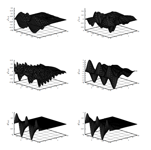
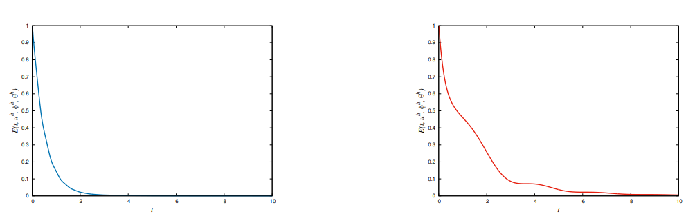
This paper provides a comprehensive analysis of the stabilization properties for the coupled poroelastic system with Type III thermoelasticity given in (7). Using semigroup theory, we have shown the existence and uniqueness of the system, as well as its exponential stability for the case where the wave propagation speeds are equal \(\dfrac{\rho}{\mu}=\dfrac{J}{\delta}\). On the other hand, the loss of exponential stability was demonstrated when the wave propagation speeds are different, \(\dfrac{\rho}{\mu}\neq\dfrac{J}{\delta}\). Furthermore, by using the Borichev-Tomilov Theorem, we successfully established that the system exhibits an optimal polynomial decay rate of \(t^{-1/2}\). These theoretical findings significantly improve upon previous results in the literature [19]. To complement this analysis, we present the construction and implementation of a numerical scheme based on the Newmark method. Our numerical experiments are in full agreement with the analytical results. Specifically, when the wave propagation speeds are equal, we obtain exponential energy decay, as illustrated in Figure 2 on the left. On the other hand, if this condition is violated, the decay rate becomes slower, a behavior captured in Figure 2 on the right. The same can be observed in Figure 1, in this case for the functions \(u,\phi,\theta\).
Silvia Santos, Sebastião Cordeiro; Conceptualization, methodology, formal analysis, investigation, writing-original draft preparation. Anderson Campelo, Carlos Raposo; Writing-review and editing, visualization, supervision, project administration. Carlos Baldez; Numerical Analysis.
The authors declare no conflict of interest.
No data is required for this research.
No funding is available for this research.
The authors thank the anonymous referees for their valuable contributions, which significantly improved this manuscript. S. Cordeiro thanks the CNPq-Brazil Grant 303608/2025-0, A. Campelo thanks the CNPq-Brazil Grant 312758/2025-1, C. Raposo thanks the CNPq-Brazil Grant 307447/2023-5.