
Quaternions were first discovered in 1843 by Sir William Rowan Hamilton. Quaternions are a generalization of complex numbers [1]. They form a four-dimensional number system and correspond to rotations in three-dimensional space. Therefore, they are widely used in vector studies and spherical geometry. Quaternions are also used in vector analysis, geometry, physics, computer animation, mechanics, and robotics.
A quaternion generally has the form \[h=a+ib+jc+kd,\] where \(i\), \(j\), and \(k\) are quaternion units, and \(a\), \(b\), \(c\), and \(d\) are real numbers. These quaternion units satisfy the multiplication rules shown in Table 1.
| \(\cdot\) | \(i\) | \(j\) | \(k\) |
|---|---|---|---|
| \(i\) | \(-1\) | \(k\) | \(-j\) |
| \(j\) | \(-k\) | \(-1\) | \(i\) |
| \(k\) | \(j\) | \(-i\) | \(-1\) |
Quaternions have been studied by many researchers in connection with number sequences, and their properties have been examined in several contexts [1– 16].
Quasi-quaternion algebra was introduced by Mehdi Jafari, who also investigated its fundamental properties [17]. Quasi-quaternions are a special type of quaternion. Unlike classical quaternions, quasi-quaternions satisfy the commutative property. A notable research direction in this field is the study of quasi-quaternions as an alternative quaternion algebra in which multiplication remains commutative. This structure provides new insights into number sequences by incorporating vector components together with the traditional scalar terms. In recent years, researchers have extended Fibonacci and Lucas sequences to quasi-quaternions, allowing a deeper understanding of their algebraic properties, recurrence relations, and generating functions.
This study introduces and analyzes Fibonacci and Lucas quasi-quaternions through various algebraic and geometric approaches. We establish their recurrence relations, generating functions, and fundamental identities. Furthermore, we use De Moivre’s formula in the quasi-quaternion setting, extending classical results to higher-order powers of these structures. A key contribution of this paper is the graphical analysis of Fibonacci and Lucas quasi-quaternions, which provides geometric interpretations of their behavior under different parameters [18, 19].
This paper extends these works by presenting graphical visualizations of Fibonacci and Lucas quasi-quaternions in §4. By analyzing their rotational properties and asymptotic behavior, we provide new insights into how these sequences behave in quasi-quaternionic space. Our results highlight the significance of De Moivre’s formula in governing the transformations of these sequences, offering a deeper understanding of their long-term stability and convergence.
The remainder of this paper is organized as follows. §2 defines Fibonacci and Lucas quasi-quaternions and presents their fundamental properties. §3 establishes De Moivre’s formula and matrix representations of these quasi-quaternions. §4 focuses on graphical analysis and its implications, particularly for understanding the geometric behavior of quasi-quaternions under iterative transformations.
We now recall the basic definitions concerning quasi-quaternions.
Definition 1. A quasi-quaternion \(q\) is defined by \[q=a_0+a_1i+a_2j+a_3k,\] where \(a_0\), \(a_1\), \(a_2\), and \(a_3\) are real numbers, and \(i\), \(j\), and \(k\) are basic vectors [17]. These basis vectors satisfy the following multiplication rules: \[i^2=j^2=k^2=0, \qquad ij=ji=jk=kj=ki=ik=0.\]
The following definitions give the real part, imaginary part, conjugate, and norm of a quasi-quaternion.
Definition 2. [17] Let \[q=a_0+a_1i+a_2j+a_3k\] be a quasi-quaternion. Then the following notions are defined as follows.
The real part of \(q\) is \[S_q=a_0,\] and the imaginary part of \(q\) is \[V_q=a_1i+a_2j+a_3k.\]
The conjugate of \(q\) is denoted by \(\overline{q}\) and is defined by \[\overline{q}=a_0-a_1i-a_2j-a_3k.\]
The norm of \(q\) is defined by \[N(q)=\|q\|=q\overline{q}.\]
Definition 3. Each nonzero quasi-quaternion \[q=a_0+a_1i+a_2j+a_3k\] can be written in polar form as follows [17]: \[q=\kappa\left(\cos\theta+\vec{v}\sin\theta\right), \qquad 0\leq \theta \leq 2\pi,\] where \[\kappa=\sqrt{N(q)}, \qquad \cos\theta=\frac{a_0}{\kappa},\] and \[\sin\theta=\theta = \frac{\sqrt{a_1^2+a_2^2+a_3^2}}{\kappa}.\] The vector \(\vec{v}\) is given by \[\vec{v} = \frac{a_1i+a_2j+a_3k} {\sqrt{a_1^2+a_2^2+a_3^2}}.\]
The occurrence of sine values greater than one in quasi-quaternion algebra is a fundamental consequence of the non-Euclidean and parabolic nature of this algebraic structure. This result is mathematically consistent and rigorous for the following reasons.
First, in quasi-quaternion algebra \(H^\circ\), the squares of the imaginary units are zero, that is, \[i^2=j^2=k^2=0.\] Unlike real quaternions, where imaginary units define a hyperspherical structure, the units in \(H^\circ\) define a linear structure consistent with Galilean space-time transformations.
Second, sine and cosine functions are defined through their power-series expansions. Due to the nilpotency of the vector part, namely \(\vec{w}^{\,2}=0\), all higher-order terms with \(n\geq 2\) in the Taylor expansions vanish. Hence, the corresponding transcendental functions reduce to the linear forms \[\cos\theta=1, \qquad \sin\theta=\theta.\]
Third, in this context, the parameter \(\theta\) does not represent a circular angle in a Euclidean plane. Instead, it represents the norm, or magnitude, of the vector part of the quasi-quaternion. Therefore, \(\sin\theta\) is directly proportional to the Euclidean norm of the spatial components and may take any real value \(\theta\in[0,\infty)\).
Finally, the norm of a quasi-quaternion is determined only by its scalar part, namely \[N_q=a_0^2.\] Since the vector part, and consequently the sine component, does not contribute to the norm, the condition \(\sin\theta>1\) does not violate the unit property of the quasi-quaternion as long as \(a_0=1\) [17].
Theorem 1(De Moivre’s formula).Let \(q\) be a unit quasi-quaternion given by \[q=e^{\vec{v}\theta} = \cos\theta+\vec{v}\sin\theta.\] Then, for every positive integer \(n\), we have \[q^n=\cos(n\theta)+\vec{v}\sin(n\theta).\]
For a quasi-quaternion \[q=a_0+a_1i+a_2j+a_3k,\] the mapping \(\theta_q:H^\circ\to H^\circ\) is defined by \[\theta_q(x)=qx, \qquad x\in H^\circ,\] where \(\theta_q\) is the Hamilton operator [17].
The matrix representation of the quasi-quaternion \(q\) is given by \[\mathcal{M}_q = \begin{pmatrix} a_0 & 0 & 0 & 0 \\ a_1 & a_0 & 0 & 0 \\ a_2 & 0 & a_0 & 0 \\ a_3 & 0 & 0 & a_0 \end{pmatrix}.\] Jafari also computed the powers of these matrices in his work [17].
Fibonacci and Lucas sequences are among the most important integer sequences. They have been widely studied and continue to be active topics of research.
These sequences have applications in group theory, linear algebra, applied mathematics, and other branches of mathematics. They also have applications in other scientific fields, such as computer science, physics, biology, and statistics.
The Fibonacci numbers are defined by [9] \[F_n=F_{n-1}+F_{n-2}, \qquad n\geq 2,\] with \[F_0=0, \qquad F_1=1.\]
The Lucas numbers are defined by \[L_n=L_{n-1}+L_{n-2}, \qquad n\geq 2,\] with \[L_0=2, \qquad L_1=1\] [9]. Moreover, \[L_{-n}=(-1)^nL_n, \qquad F_{-n}=(-1)^{n+1}F_n.\]
We now recall the Fibonacci and Lucas identities used in this study.
Theorem 2. The following relations hold [9]: \[\begin{aligned} \boldsymbol{a}. &\qquad F_{n-1}+F_{n+1}=L_n, && n\geq 1,\\ \boldsymbol{b}. &\qquad F_{n+2}-F_{n-2}=L_n, && n\geq 2,\\ \boldsymbol{c}. &\qquad L_{n-1}+L_{n+1}=5F_n, && n\geq 1,\\ \boldsymbol{d}. &\qquad L_{n+2}-L_{n-2}=5F_n, && n\geq 2,\\ \boldsymbol{e}. &\qquad F_nL_n=F_{2n}, && n\geq 0. \end{aligned}\]
Theorem 3.[7] For \(n,r,s\geq 0\), we have \[F_{n+r}L_{n+s} = F_{2n+r+s} + (-1)^{n+s+1}F_{r-s}.\]
Theorem 4. [9] The sums of Fibonacci and Lucas numbers are given as follows: \[\begin{aligned} \boldsymbol{a}. &\qquad \sum_{i=1}^{n}F_i=F_{n+2}-1,\\ \boldsymbol{b}. &\qquad \sum_{i=1}^{n}L_i=L_{n+2}-3. \end{aligned}\]
In this study, we define a new application of quasi-quaternions by taking the real coefficients of quasi-quaternions from Fibonacci and Lucas numbers. We refer to these objects as Fibonacci quasi-quaternions and Lucas quasi-quaternions. We examine their properties and present several important identities.
In this section, we define Fibonacci and Lucas quasi-quaternions and introduce some identities involving them. Throughout the article, we denote the quasi-quaternion units \(i\), \(j\), and \(k\) by \(e_1\), \(e_2\), and \(e_3\), respectively.
Definition 4. The Fibonacci and Lucas quasi-quaternions are defined by \[\begin{aligned} QF_n &=F_n+F_{n+1}e_1+F_{n+2}e_2+F_{n+3}e_3 \\ &=(F_n,F_{n+1},F_{n+2},F_{n+3}), \end{aligned}\] and \[\begin{aligned} QL_n &=L_n+L_{n+1}e_1+L_{n+2}e_2+L_{n+3}e_3 \\ &=(L_n,L_{n+1},L_{n+2},L_{n+3}), \end{aligned}\] where \(F_n\) and \(L_n\) are the \(n\)th Fibonacci and Lucas numbers, respectively, and \(e_1\), \(e_2\), and \(e_3\) are quasi-quaternion units. These basis vectors satisfy the multiplication rules given in Definition 1.
Some terms of the Fibonacci and Lucas quasi-quaternions are given in Tables 2 and 3, respectively.
| \(\boldsymbol{n}\) | \(\boldsymbol{QF_n}\) |
|---|---|
| \(0\) | \(e_1+e_2+2e_3\) |
| \(1\) | \(1+e_1+2e_2+3e_3\) |
| \(2\) | \(1+2e_1+3e_2+5e_3\) |
| \(3\) | \(2+3e_1+5e_2+8e_3\) |
| \(4\) | \(3+5e_1+8e_2+13e_3\) |
| \(\boldsymbol{n}\) | \(\boldsymbol{QL_n}\) |
|---|---|
| \(0\) | \(2+e_1+3e_2+4e_3\) |
| \(1\) | \(1+3e_1+4e_2+7e_3\) |
| \(2\) | \(3+4e_1+7e_2+11e_3\) |
| \(3\) | \(4+7e_1+11e_2+18e_3\) |
| \(4\) | \(7+11e_1+18e_2+29e_3\) |
Definition 5. For \(n\geq 1\), the Fibonacci and Lucas quasi-quaternions with negative indices are defined by \[\begin{aligned} QF_{-n} &= (-1)^n\left(-F_n+F_{n-1}e_1-F_{n-2}e_2+F_{n-3}e_3\right), \\ QL_{-n} &= (-1)^n\left(L_n-L_{n-1}e_1+L_{n-2}e_2-L_{n-3}e_3\right), \end{aligned}\] where \(F_n\) and \(L_n\) are the \(n\)th Fibonacci and Lucas numbers, respectively, and \(e_1\), \(e_2\), and \(e_3\) are quasi-quaternion units. These basis vectors satisfy the multiplication rules given in Definition 1.
Definition 6. The real and imaginary parts of the Fibonacci and Lucas quasi-quaternions are given, respectively, by \[\begin{aligned} \operatorname{Re}(QF_n)&=F_n, & \operatorname{Im}(QF_n)&=F_{n+1}e_1+F_{n+2}e_2+F_{n+3}e_3, \\ \operatorname{Re}(QL_n)&=L_n, & \operatorname{Im}(QL_n)&=L_{n+1}e_1+L_{n+2}e_2+L_{n+3}e_3. \end{aligned}\]
Definition 7. The conjugates of \(QF_n\) and \(QL_n\) are denoted by \(\overline{QF}_n\) and \(\overline{QL}_n\), respectively, and are defined as follows: \[\begin{aligned} \boldsymbol{a}. \quad \overline{QF}_n &= F_n-F_{n+1}e_1-F_{n+2}e_2-F_{n+3}e_3, \\ \boldsymbol{b}. \quad \overline{QL}_n &= L_n-L_{n+1}e_1-L_{n+2}e_2-L_{n+3}e_3. \end{aligned}\]
Theorem 5.The norms of \(QF_n\) and \(QL_n\) are given by \[\begin{aligned} \boldsymbol{a}. \quad & N(QF_n)=F_n^2, \\ \boldsymbol{b}. \quad & N(QL_n)=L_n^2. \end{aligned}\]
Proof. For \(\boldsymbol{a}\), we have \[\begin{aligned} N(QF_n) &=QF_n\overline{QF}_n \\ &= \left(F_n+F_{n+1}e_1+F_{n+2}e_2+F_{n+3}e_3\right) \left(F_n-F_{n+1}e_1-F_{n+2}e_2-F_{n+3}e_3\right). \end{aligned}\] Using the multiplication rules of \(e_1\), \(e_2\), and \(e_3\), we obtain \[N(QF_n)=F_n^2.\] Thus, the proof is completed. The proof of \(\boldsymbol{b}\) is similar to that of \(\boldsymbol{a}\). ◻
Example 1. The quasi-quaternions \(QF_1\) and \(QF_2\) are unit quasi-quaternions, since \[N(QF_1)=N(QF_2)=1.\]
Theorem 6. The Fibonacci and Lucas quasi-quaternions satisfy the following recurrence relations: \[\begin{aligned} \boldsymbol{a}. \quad & QF_n=QF_{n-1}+QF_{n-2}, && n\geq 2, \\ \boldsymbol{b}. \quad & QL_n=QL_{n-1}+QL_{n-2}, && n\geq 2. \end{aligned}\]
Proof. We use the recurrence relation of the Fibonacci numbers. We have \[\begin{aligned} QF_n &=F_n+F_{n+1}e_1+F_{n+2}e_2+F_{n+3}e_3 \\ &=F_{n-1}+F_{n-2} +\left(F_n+F_{n-1}\right)e_1 +\left(F_{n+1}+F_n\right)e_2 +\left(F_{n+2}+F_{n+1}\right)e_3 \\ &= \left(F_{n-1}+F_ne_1+F_{n+1}e_2+F_{n+2}e_3\right) +\left(F_{n-2}+F_{n-1}e_1+F_ne_2+F_{n+1}e_3\right) \\ &=QF_{n-1}+QF_{n-2}. \end{aligned}\] Thus, the proof is completed. The proof of \(\boldsymbol{b}\) is similar to that of \(\boldsymbol{a}\). ◻
The next theorem gives the relationship among Fibonacci quasi-quaternions, Lucas quasi-quaternions, Fibonacci numbers, and Lucas numbers.
Theorem 7. For \(n\geq 1\), the following identities hold: \[\begin{aligned} \boldsymbol{a}. \quad & QF_{n-1}+QF_{n+1}=QL_n, \\ \boldsymbol{b}. \quad & QF_{n+2}-QF_{n-2}=QL_n, \\ \boldsymbol{c}. \quad & QL_{n-1}+QL_{n+1}=5QF_n, \\ \boldsymbol{d}. \quad & QL_{n+2}-QL_{n-2}=5QF_n, \\ \boldsymbol{e}. \quad & QF_nQL_n=2QF_{2n}-F_{2n}, \\ \boldsymbol{f}. \quad & QF_{n+1}^2+QF_n^2 =F_{n+1}\left(2QF_{n+1}-F_{n+1}\right), \\ \boldsymbol{g}. \quad & QF_n-e_1QF_{n+1}-e_2QF_{n+2}-e_3QF_{n+3}=F_n, \\ \boldsymbol{h}. \quad & QF_n+e_1QF_{n+3}+e_2QF_{n+4}+e_3QF_{n+5} =QL_{n+1}-F_{n+2}, \\ \boldsymbol{i}. \quad & QF_{n+r}L_{n+r} =QF_{2n+2r}+(-1)^{n+r}QF_0. \end{aligned}\]
Proof. For \(\boldsymbol{a}\), we have \[\begin{aligned} QF_{n-1}+QF_{n+1} &= \left(F_{n-1}+F_ne_1+F_{n+1}e_2+F_{n+2}e_3\right) \\ &\quad+ \left(F_{n+1}+F_{n+2}e_1+F_{n+3}e_2+F_{n+4}e_3\right) \\ &= \left(F_{n-1}+F_{n+1}\right) +\left(F_n+F_{n+2}\right)e_1 \\ &\quad+ \left(F_{n+1}+F_{n+3}\right)e_2 +\left(F_{n+2}+F_{n+4}\right)e_3. \end{aligned}\] Using Theorem 2\(\boldsymbol{a}\), we obtain \[QF_{n-1}+QF_{n+1} = L_n+L_{n+1}e_1+L_{n+2}e_2+L_{n+3}e_3 = QL_n.\]
For \(\boldsymbol{e}\), we have \[\begin{aligned} QF_nQL_n &= \left(F_n+F_{n+1}e_1+F_{n+2}e_2+F_{n+3}e_3\right) \left(L_n+L_{n+1}e_1+L_{n+2}e_2+L_{n+3}e_3\right) \\ &= F_nL_n +\left(F_nL_{n+1}+F_{n+1}L_n\right)e_1 \\ &\quad+ \left(F_nL_{n+2}+F_{n+2}L_n\right)e_2 +\left(F_nL_{n+3}+F_{n+3}L_n\right)e_3. \end{aligned}\] By Theorem 2\(\boldsymbol{e}\) and Theorem 3, it follows that \[\begin{aligned} QF_nQL_n &= F_{2n} +2F_{2n+1}e_1 +2F_{2n+2}e_2 +2F_{2n+3}e_3 \\ &= 2QF_{2n}-F_{2n}. \end{aligned}\] Thus, the proof is completed. The remaining identities can be proved similarly. ◻
Theorem 8(Binet Formulas).Let \[a=\frac{1+\sqrt{5}}{2}, \qquad b=\frac{1-\sqrt{5}}{2},\] and define \[\hat{a}=1+ae_1+a^2e_2+a^3e_3, \qquad \hat{b}=1+be_1+b^2e_2+b^3e_3.\] Then, for \(n\geq 0\), we have \[\begin{aligned} \boldsymbol{a}. \quad QF_n &= \frac{a^n\hat{a}-b^n\hat{b}}{\sqrt{5}}, \\ \boldsymbol{b}. \quad QL_n &= a^n\hat{a}+b^n\hat{b}, \\ \boldsymbol{c}. \quad QF_{-n} &= \frac{b^n\hat{a}-a^n\hat{b}}{\sqrt{5}(-1)^n}, \\ \boldsymbol{d}. \quad QL_{-n} &= \frac{b^n\hat{a}+a^n\hat{b}}{(-1)^n}. \end{aligned}\]
Proof. We use the Binet formula for the Fibonacci numbers. For \(\boldsymbol{a}\), we obtain \[\begin{aligned} QF_n &= F_n+F_{n+1}e_1+F_{n+2}e_2+F_{n+3}e_3 \\ &= \left(\frac{a^n-b^n}{\sqrt{5}}\right) +\left(\frac{a^{n+1}-b^{n+1}}{\sqrt{5}}\right)e_1 +\left(\frac{a^{n+2}-b^{n+2}}{\sqrt{5}}\right)e_2 +\left(\frac{a^{n+3}-b^{n+3}}{\sqrt{5}}\right)e_3 \\ &= \frac{a^n\left(1+ae_1+a^2e_2+a^3e_3\right)}{\sqrt{5}} – \frac{b^n\left(1+be_1+b^2e_2+b^3e_3\right)}{\sqrt{5}} \\ &= \frac{a^n\hat{a}-b^n\hat{b}}{\sqrt{5}}. \end{aligned}\] Thus, the proof is completed. The remaining formulas can be proved similarly. ◻
Theorem 9(Generating Functions).The generating functions of \(QF_n\) and \(QL_n\) are given by \[\begin{aligned} \boldsymbol{a}. \quad \sum_{n=0}^{\infty}QF_nx^n &= \frac{QF_0+\left(QF_1-QF_0\right)x}{1-x-x^2}, \\ \boldsymbol{b}. \quad \sum_{n=0}^{\infty}QL_nx^n &= \frac{QL_0+\left(QL_1-QL_0\right)x}{1-x-x^2}. \end{aligned}\]
Proof. Let \[ G(x)=\sum_{n=0}^{\infty}QF_nx^n=QF_0+QF_1x+QF_2x^2+QF_3x^3+\cdots+QF_nx^n+\cdots .\qquad\qquad \qquad\qquad (1)\]
Multiplying (1) by \(x\) and \(x^2\), respectively, gives \[xG(x)=QF_0x+QF_1x^2+QF_2x^3+QF_3x^4+\cdots,\] and \[x^2G(x)=QF_0x^2+QF_1x^3+QF_2x^4+QF_3x^5+\cdots.\] Using the recurrence relation and subtracting the last two equations from (1), we obtain \[G(x)(1-x-x^2)=QF_0+QF_1x-QF_0x.\] Therefore, \[G(x)= \frac{QF_0+\left(QF_1-QF_0\right)x}{1-x-x^2}.\] Thus, the proof is completed. The proof of \(\boldsymbol{b}\) is similar. ◻
Theorem 10(Exponential Generating Functions).The exponential generating functions of \(QF_n\) and \(QL_n\) are given by \[\begin{aligned} \boldsymbol{a}. \quad \sum_{n=0}^{\infty}QF_n\frac{x^n}{n!} &= \frac{\hat{a}e^{ax}-\hat{b}e^{bx}}{\sqrt{5}}, \\ \boldsymbol{b}. \quad \sum_{n=0}^{\infty}QL_n\frac{x^n}{n!} &= \hat{a}e^{ax}+\hat{b}e^{bx}. \end{aligned}\]
Proof. For \(\boldsymbol{a}\), we use the Binet formula for Fibonacci quasi-quaternions: \[\begin{aligned} \sum_{n=0}^{\infty}QF_n\frac{x^n}{n!} &= \sum_{n=0}^{\infty} \left(\frac{a^n\hat{a}-b^n\hat{b}}{\sqrt{5}}\right) \frac{x^n}{n!} \\ &= \frac{\hat{a}}{\sqrt{5}} \sum_{n=0}^{\infty}\frac{(ax)^n}{n!} – \frac{\hat{b}}{\sqrt{5}} \sum_{n=0}^{\infty}\frac{(bx)^n}{n!}. \end{aligned}\] Since \[\sum_{n=0}^{\infty}\frac{x^n}{n!}=e^x,\] we obtain \[\sum_{n=0}^{\infty}QF_n\frac{x^n}{n!} = \frac{\hat{a}e^{ax}-\hat{b}e^{bx}}{\sqrt{5}}.\] Thus, the proof is completed. The proof of \(\boldsymbol{b}\) is similar. ◻
Theorem 11(Sum Formulas).The following sum formulas hold: \[\begin{aligned} \boldsymbol{a}. \quad \sum_{i=1}^{n}QF_i &= QF_{n+2}-QF_0-QF_1, \\ \boldsymbol{b}. \quad \sum_{i=1}^{n}QL_i &= QL_{n+2}-QL_0-QL_1. \end{aligned}\]
Proof. We use the sum formula for the Fibonacci numbers. For \(\boldsymbol{a}\), we have \[\begin{aligned} \sum_{i=1}^{n}QF_i &= \sum_{i=1}^{n} \left(F_i+F_{i+1}e_1+F_{i+2}e_2+F_{i+3}e_3\right) \\ &= \sum_{i=1}^{n}F_i +e_1\sum_{i=1}^{n}F_{i+1} +e_2\sum_{i=1}^{n}F_{i+2} +e_3\sum_{i=1}^{n}F_{i+3}. \end{aligned}\] By Theorem 4, we obtain \[\begin{aligned} \sum_{i=1}^{n}QF_i &= F_{n+2}-1 +e_1\left(F_{n+3}-1-F_1\right) +e_2\left(F_{n+4}-1-F_1-F_2\right) \\ &\quad +e_3\left(F_{n+5}-1-F_1-F_2-F_3\right) \\ &= F_{n+2}+F_{n+3}e_1+F_{n+4}e_2+F_{n+5}e_3 \\ &\quad -\left(F_0+F_1e_1+F_2e_2+F_3e_3\right) -\left(F_1+F_2e_1+F_3e_2+F_4e_3\right) \\ &= QF_{n+2}-QF_0-QF_1. \end{aligned}\] Thus, the desired formula is obtained. The proof of \(\boldsymbol{b}\) is similar. ◻
Lemma 1. The following identities hold: \[\begin{aligned} \boldsymbol{a}. \quad & \hat{a}\hat{b}=\hat{a}+\hat{b}-1, \\ \boldsymbol{b}. \quad & \hat{a}^{\,2}=2\hat{a}-1, \\ \boldsymbol{c}. \quad & \hat{b}^{\,2}=2\hat{b}-1. \end{aligned}\]
Theorem 12(Cassini Identities).For \(n\geq 1\), the following identities hold: \[\begin{aligned} \boldsymbol{a}. \quad QF_{n-1}QF_{n+1}-QF_n^2 &= (-1)^n\hat{a}\hat{b}, \\ \boldsymbol{b}. \quad QL_{n-1}QL_{n+1}-QL_n^2 &= 5(-1)^{n-1}\hat{a}\hat{b}. \end{aligned}\]
Proof. For \(\boldsymbol{a}\), we use the Binet formula for Fibonacci quasi-quaternions: \[\begin{aligned} QF_{n-1}QF_{n+1}-QF_n^2 &= \left(\frac{a^{n-1}\hat{a}-b^{n-1}\hat{b}}{\sqrt{5}}\right) \left(\frac{a^{n+1}\hat{a}-b^{n+1}\hat{b}}{\sqrt{5}}\right) \\ &\quad – \left(\frac{a^n\hat{a}-b^n\hat{b}}{\sqrt{5}}\right)^2 \\ &= \frac{ -a^{n-1}b^{n+1}\hat{a}\hat{b} -b^{n-1}a^{n+1}\hat{b}\hat{a} +a^nb^n\hat{a}\hat{b} +b^na^n\hat{b}\hat{a} }{5}. \end{aligned}\] Using Lemma 1, we get \[\begin{aligned} QF_{n-1}QF_{n+1}-QF_n^2 &= \frac{a^{n-1}b^{n-1}\hat{a}\hat{b}}{5} \left(2ab-a^2-b^2\right) \\ &= \frac{-(ab)^{n-1}\hat{a}\hat{b}(a-b)^2}{5}. \end{aligned}\] Since \(a-b=\sqrt{5}\) and \(ab=-1\), we obtain \[QF_{n-1}QF_{n+1}-QF_n^2 = (-1)^n\hat{a}\hat{b}.\] Thus, the desired identity is obtained. The proof of \(\boldsymbol{b}\) is similar. ◻
Theorem 13(Catalan Identities).For \(n\geq t\), the following identities hold: \[\begin{aligned} \boldsymbol{a}. \quad QF_{n-t}QF_{n+t}-QF_n^2 &= (-1)^{n-t+1}F_t^2\hat{a}\hat{b}, \\ \boldsymbol{b}. \quad QL_{n-t}QL_{n+t}-QL_n^2 &= 5(-1)^{n-t}F_t^2\hat{a}\hat{b}. \end{aligned}\]
Proof. For \(\boldsymbol{a}\), we use the Binet formula for Fibonacci quasi-quaternions: \[\begin{aligned} QF_{n-t}QF_{n+t}-QF_n^2 &= \left(\frac{a^{n-t}\hat{a}-b^{n-t}\hat{b}}{\sqrt{5}}\right) \left(\frac{a^{n+t}\hat{a}-b^{n+t}\hat{b}}{\sqrt{5}}\right) \\ &\quad – \left(\frac{a^n\hat{a}-b^n\hat{b}}{\sqrt{5}}\right)^2 \\ &= \frac{ -a^{n-t}b^{n+t}\hat{a}\hat{b} -b^{n-t}a^{n+t}\hat{b}\hat{a} +a^nb^n\hat{a}\hat{b} +b^na^n\hat{b}\hat{a} }{5}. \end{aligned}\] Using Lemma 1, we obtain \[\begin{aligned} QF_{n-t}QF_{n+t}-QF_n^2 &= \frac{a^nb^n\hat{a}\hat{b}}{5} \left( 2-\left(\frac{b}{a}\right)^t-\left(\frac{a}{b}\right)^t \right) \\ &= \frac{-(ab)^n\hat{a}\hat{b}(a^t-b^t)^2} {(a-b)^2(ab)^t}. \end{aligned}\] Since \(ab=-1\) and \[F_t=\frac{a^t-b^t}{a-b},\] we get \[QF_{n-t}QF_{n+t}-QF_n^2 = (-1)^{n-t+1}F_t^2\hat{a}\hat{b}.\] Thus, the desired identity is obtained. The proof of \(\boldsymbol{b}\) is similar. ◻
Theorem 14(d’Ocagne Identities).For \(n,m\in\mathbb{Z}\), the following identities hold: \[\begin{aligned} \boldsymbol{a}. \quad QF_mQF_{n+1}-QF_nQF_{m+1} &= (-1)^n\hat{a}\hat{b}F_{m-n}, \\ \boldsymbol{b}. \quad QL_mQL_{n+1}-QL_nQL_{m+1} &= (-1)^{n+1}\sqrt{5}\,\hat{a}\hat{b}F_{m-n}. \end{aligned}\]
Proof. For \(\boldsymbol{a}\), we use the Binet formula for Fibonacci quasi-quaternions: \[\begin{aligned} QF_mQF_{n+1}-QF_nQF_{m+1} &= \left(\frac{a^m\hat{a}-b^m\hat{b}}{\sqrt{5}}\right) \left(\frac{a^{n+1}\hat{a}-b^{n+1}\hat{b}}{\sqrt{5}}\right) \\ &\quad – \left(\frac{a^n\hat{a}-b^n\hat{b}}{\sqrt{5}}\right) \left(\frac{a^{m+1}\hat{a}-b^{m+1}\hat{b}}{\sqrt{5}}\right) \\ &= \frac{ -a^mb^{n+1}\hat{a}\hat{b} -b^ma^{n+1}\hat{b}\hat{a} +a^nb^{m+1}\hat{a}\hat{b} +b^na^{m+1}\hat{b}\hat{a} }{5}. \end{aligned}\] Using Lemma 1, we obtain \[\begin{aligned} QF_mQF_{n+1}-QF_nQF_{m+1} &= \frac{a^mb^n\hat{a}\hat{b}(a-b) -a^nb^m\hat{a}\hat{b}(a-b)}{5} \\ &= \frac{\hat{a}\hat{b}(a-b)(a^mb^n-a^nb^m)}{5} \\ &= \frac{\hat{a}\hat{b}(a-b)a^nb^n(a^{m-n}-b^{m-n})}{5}. \end{aligned}\] Since \(ab=-1\) and \[F_t=\frac{a^t-b^t}{a-b},\] we get \[QF_mQF_{n+1}-QF_nQF_{m+1} = (-1)^n\hat{a}\hat{b}F_{m-n}.\] Thus, the desired identity is obtained. The proof of \(\boldsymbol{b}\) is similar. ◻
Theorem 15(Vajda Identities).For \(n,k,r\in\mathbb{Z}\), the following identities hold: \[\begin{aligned} \boldsymbol{a}. \quad QF_{n+k}QF_{n+r}-QF_nQF_{n+r+k} &= \hat{a}\hat{b}(-1)^nF_kF_r, \\ \boldsymbol{b}. \quad QL_{n+k}QL_{n+r}-QL_nQL_{n+r+k} &= 5\hat{a}\hat{b}(-1)^{n+1}F_kF_r. \end{aligned}\]
Proof. For \(\boldsymbol{a}\), we use the Binet formula for Fibonacci quasi-quaternions: \[\begin{aligned} QF_{n+k}QF_{n+r}-QF_nQF_{n+r+k} &= \left(\frac{a^{n+k}\hat{a}-b^{n+k}\hat{b}}{\sqrt{5}}\right) \left(\frac{a^{n+r}\hat{a}-b^{n+r}\hat{b}}{\sqrt{5}}\right) \\ &\quad – \left(\frac{a^n\hat{a}-b^n\hat{b}}{\sqrt{5}}\right) \left(\frac{a^{n+r+k}\hat{a}-b^{n+r+k}\hat{b}}{\sqrt{5}}\right) \\ &= \frac{ -a^{n+k}b^{n+r}\hat{a}\hat{b} -b^{n+k}a^{n+r}\hat{b}\hat{a} +a^nb^{n+r+k}\hat{a}\hat{b} +b^na^{n+r+k}\hat{b}\hat{a} }{5}. \end{aligned}\] Using Lemma 1, we have \[\begin{aligned} QF_{n+k}QF_{n+r}-QF_nQF_{n+r+k} &= \frac{\hat{a}\hat{b} \left[ a^nb^{n+r}(b^k-a^k) +a^{n+r}b^n(a^k-b^k) \right]}{5}. \end{aligned}\] Since \(ab=-1\) and \[F_t=\frac{a^t-b^t}{a-b},\] we obtain \[QF_{n+k}QF_{n+r}-QF_nQF_{n+r+k} = \hat{a}\hat{b}(-1)^nF_kF_r.\] Thus, the desired identity is obtained. The proof of \(\boldsymbol{b}\) is similar. ◻
Theorem 16(Honsberger Identities).For \(n,m\in\mathbb{Z}\), the following identities hold: \[\begin{aligned} \boldsymbol{a}. \quad QF_{m-1}QF_n+QF_mQF_{n+1} &= \frac{ 2\left(QL_{m+n-1}+QL_{m+n+1}\right) -L_{m+n-1}-L_{m+n+1} }{5}, \\ \boldsymbol{b}. \quad QL_{m-1}QL_n+QL_mQL_{n+1} &= 2\left(QL_{m+n-1}+QL_{m+n+1}\right) -L_{m+n-1}-L_{m+n+1}. \end{aligned}\]
Proof. We prove \(\boldsymbol{a}\); the proof of \(\boldsymbol{b}\) is similar. Using the Binet formulas, we have \[\begin{aligned} QF_{m-1}QF_n+QF_mQF_{n+1} &= \left(\frac{a^{m-1}\hat{a}-b^{m-1}\hat{b}}{\sqrt{5}}\right) \left(\frac{a^n\hat{a}-b^n\hat{b}}{\sqrt{5}}\right) \\ &\quad+ \left(\frac{a^m\hat{a}-b^m\hat{b}}{\sqrt{5}}\right) \left(\frac{a^{n+1}\hat{a}-b^{n+1}\hat{b}}{\sqrt{5}}\right) \\ &= \frac{ a^{m+n-1}\hat{a}^{\,2} -a^{m-1}b^n\hat{a}\hat{b} -b^{m-1}a^n\hat{b}\hat{a} +b^{m+n-1}\hat{b}^{\,2} }{5} \\ &\quad+ \frac{ a^{m+n+1}\hat{a}^{\,2} -a^mb^{n+1}\hat{a}\hat{b} -b^ma^{n+1}\hat{b}\hat{a} +b^{m+n+1}\hat{b}^{\,2} }{5}. \end{aligned}\] By collecting terms, we obtain \[\begin{aligned} QF_{m-1}QF_n+QF_mQF_{n+1} &= \frac{ a^{m+n-1}\hat{a}^{\,2} +b^{m+n-1}\hat{b}^{\,2} +a^{m+n+1}\hat{a}^{\,2} +b^{m+n+1}\hat{b}^{\,2} }{5} \\ &\quad+ \frac{ -a^{m-1}b^n\hat{a}\hat{b}(1+ab) -b^{m-1}a^n\hat{b}\hat{a}(1+ab) }{5}. \end{aligned}\] Since \(ab=-1\), the second fraction vanishes. Therefore, using Lemma 1, we get \[\begin{aligned} QF_{m-1}QF_n+QF_mQF_{n+1} &= \frac{ a^{m+n-1}(2\hat{a}-1) +b^{m+n-1}(2\hat{b}-1) }{5} \\ &\quad+ \frac{ a^{m+n+1}(2\hat{a}-1) +b^{m+n+1}(2\hat{b}-1) }{5} \\ &= \frac{ 2\left(a^{m+n-1}\hat{a}+b^{m+n-1}\hat{b}\right) -\left(a^{m+n-1}+b^{m+n-1}\right) }{5} \\ &\quad+ \frac{ 2\left(a^{m+n+1}\hat{a}+b^{m+n+1}\hat{b}\right) -\left(a^{m+n+1}+b^{m+n+1}\right) }{5} \\ &= \frac{ 2\left(QL_{m+n-1}+QL_{m+n+1}\right) -L_{m+n-1}-L_{m+n+1} }{5}. \end{aligned}\] Thus, the proof is completed. ◻
Each Fibonacci quasi-quaternion \(QF_n\) and Lucas quasi-quaternion \(QL_n\) can be written in polar form. For \(QF_n\), we write \[QF_n=\kappa_n\left(\cos\theta_n+\vec{t}_n\sin\theta_n\right), \qquad \kappa_n=\sqrt{N(QF_n)}.\] Similarly, for \(QL_n\), we write \[QL_n=\rho_n\left(\cos\vartheta_n+\vec{d}_n\sin\vartheta_n\right), \qquad \rho_n=\sqrt{N(QL_n)}.\] For the Fibonacci quasi-quaternion, the unit vector \(\vec{t}_n\) is given by \[\vec{t}_n = \frac{ F_{n+1}e_1+F_{n+2}e_2+F_{n+3}e_3 } { \sqrt{F_{n+1}^2+F_{n+2}^2+F_{n+3}^2} },\] and \[\cos\theta_n=\frac{F_n}{\kappa_n}, \qquad \sin\theta_n=\theta_n = \frac{ \sqrt{F_{n+1}^2+F_{n+2}^2+F_{n+3}^2} } {\kappa_n}.\] Similarly, for the Lucas quasi-quaternion, we have \[\vec{d}_n = \frac{ L_{n+1}e_1+L_{n+2}e_2+L_{n+3}e_3 } { \sqrt{L_{n+1}^2+L_{n+2}^2+L_{n+3}^2} },\] and \[\cos\vartheta_n=\frac{L_n}{\rho_n}, \qquad \sin\vartheta_n=\vartheta_n = \frac{ \sqrt{L_{n+1}^2+L_{n+2}^2+L_{n+3}^2} } {\rho_n}.\]
We now give an example of the above polar representation.
Example 2. For \[QF_2=1+2e_1+3e_2+5e_3,\] we have \[\kappa_2=\sqrt{N(QF_2)}=1.\] Moreover, \[\vec{t}_2 = \frac{2e_1+3e_2+5e_3}{\sqrt{2^2+3^2+5^2}} = \frac{2e_1+3e_2+5e_3}{\sqrt{38}},\] and \[\cos\theta_2=\frac{1}{1}=1, \qquad \sin\theta_2=\theta_2=\frac{\sqrt{38}}{1}=\sqrt{38}.\] Thus, \[\begin{aligned} QF_2 &= \kappa_2\left(\cos\theta_2+\vec{t}_2\sin\theta_2\right) \\ &= 1+\frac{2e_1+3e_2+5e_3}{\sqrt{38}}\sqrt{38} \\ &= 1+2e_1+3e_2+5e_3. \end{aligned}\]
Theorem 17(De Moivre’s Formula).Let \[QF_n=e^{\vec{t}\theta}=\cos\theta+\vec{t}\sin\theta.\] Then, for every integer \(k\), we have \[QF_n^k=\cos(k\theta)+\vec{t}\sin(k\theta).\] Similarly, if \[QL_n=e^{\vec{d}\vartheta} = \cos\vartheta+\vec{d}\sin\vartheta,\] then \[QL_n^k=\cos(k\vartheta)+\vec{d}\sin(k\vartheta).\]
Proof. The proof follows by induction on nonnegative integers \(k\). Assume that \[QF_n^k=\cos(k\theta)+\vec{t}\sin(k\theta).\] Then \[\begin{aligned} QF_n^{k+1} &= \left(\cos(k\theta)+\vec{t}\sin(k\theta)\right) \left(\cos\theta+\vec{t}\sin\theta\right) \\ &= \cos((k+1)\theta)+\vec{t}\sin((k+1)\theta). \end{aligned}\] Hence, the formula holds. The Lucas case is obtained similarly. ◻
We now present matrix representations of Fibonacci and Lucas quasi-quaternions and calculate the powers of these matrices.
For the Fibonacci quasi-quaternion, define the mapping \[\theta_{QF_n}:H^\circ\to H^\circ\] by \[\theta_{QF_n}(x)=QF_nx, \qquad x\in H^\circ,\] where \(\theta_{QF_n}\) is the Hamilton operator. Similarly, for the Lucas quasi-quaternion, define \[\theta_{QL_n}:H^\circ\to H^\circ\] by \[\theta_{QL_n}(x)=QL_nx, \qquad x\in H^\circ.\]
The matrix representations of the Fibonacci and Lucas quasi-quaternions are given by \[\mathcal{M}_{QF_n} = \begin{bmatrix} F_n & 0 & 0 & 0 \\ F_{n+1} & F_n & 0 & 0 \\ F_{n+2} & 0 & F_n & 0 \\ F_{n+3} & 0 & 0 & F_n \end{bmatrix},\] and \[\mathcal{M}_{QL_n} = \begin{bmatrix} L_n & 0 & 0 & 0 \\ L_{n+1} & L_n & 0 & 0 \\ L_{n+2} & 0 & L_n & 0 \\ L_{n+3} & 0 & 0 & L_n \end{bmatrix}.\]
Theorem 18. For every positive integer \(k\), we have \[\left(\mathcal{M}_{QF_n}\right)^k = F_n^{k-1} \begin{bmatrix} F_n & 0 & 0 & 0 \\ kF_{n+1} & F_n & 0 & 0 \\ kF_{n+2} & 0 & F_n & 0 \\ kF_{n+3} & 0 & 0 & F_n \end{bmatrix},\] and \[\left(\mathcal{M}_{QL_n}\right)^k = L_n^{k-1} \begin{bmatrix} L_n & 0 & 0 & 0 \\ kL_{n+1} & L_n & 0 & 0 \\ kL_{n+2} & 0 & L_n & 0 \\ kL_{n+3} & 0 & 0 & L_n \end{bmatrix}.\]
Proof. The proof follows by induction on \(k\). Equivalently, each matrix can be written as the sum of a scalar diagonal matrix and a nilpotent matrix whose square is zero. Therefore, applying the binomial formula gives the stated expressions. ◻
Quasi-quaternions based on Fibonacci and Lucas numbers provide a useful way to study quaternionic structures through matrix representations and De Moivre’s formula. In this section, we present graphical visualizations that illustrate the geometric and algebraic properties of these quasi-quaternions. By using the recursive nature of Fibonacci and Lucas sequences, we analyze the behavior of the quasi-quaternion components, including their rotational characteristics and norm variations. These graphical representations provide insight into the structure and transformations of Fibonacci and Lucas quasi-quaternions and support a deeper understanding of their mathematical properties.
In this section, we present graphical representations of Fibonacci and Lucas quasi-quaternions. We plot the quantity \[R_n = \frac{ \sqrt{F_{n+1}^2+F_{n+2}^2+F_{n+3}^2} } {F_n},\] as a function of \(n\). This ratio represents the relative contribution of the vector part to the scalar part of \(QF_n\).
Significance of the observed graphical behavior. The graphical behavior observed in the analysis of Fibonacci and Lucas numbers together with trigonometric functions provides useful insights into both theoretical and applied mathematical contexts, as shown in Figure 1. The possible scientific implications and benefits of this behavior are described below.
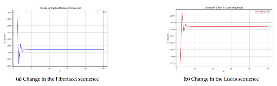
Understanding asymptotic behavior in mathematical modeling. The graph reveals the asymptotic behavior of Fibonacci- and Lucas-based functions, especially as \(n\) becomes large. As the Fibonacci numbers grow, the ratio inside the arctangent function approaches a constant, and therefore the function itself approaches a fixed value. This observation is important in mathematical modeling because it demonstrates how rapidly growing sequences, such as the Fibonacci sequence, affect the behavior of trigonometric functions, particularly in systems involving natural exponential growth patterns.
Fluctuation movement. The fluctuation movement is most visible among the first ten values, that is, for \(0<n<10\). Fibonacci numbers increase rapidly as \(n\) becomes larger. This causes the term \(F_n\) in the denominator to reach larger values, while the numerator also grows through the vector components. Initially, this produces a pronounced fluctuating movement. In other words, as \(n\) increases, the rate of change in the function \[\arctan\left( \frac{ \sqrt{F_{n+1}^2+F_{n+2}^2+F_{n+3}^2} } {F_n} \right)\] changes rapidly.
The fluctuations in the graph are mainly due to the rapidly increasing magnitudes of the Fibonacci numbers. As the expression \[\sqrt{F_{n+1}^2+F_{n+2}^2+F_{n+3}^2}\] and the denominator \(F_n\) grow in a related manner, their ratio begins to approach a constant value. Therefore, the arctangent function changes rapidly at the beginning but starts to approach a constant after a certain point.
When \(n>10\), the ratio in the formula approaches a constant value. In this case, as \(F_n\) grows, the relative variations in the numerator become smaller in comparison with the overall growth pattern, causing the function to approach a fixed limiting value.
On the other hand, Figure 2 shows that both Fibonacci and Lucas numbers increase exponentially as \(n\) increases. This is consistent with the well-known recurrence relations that define these sequences. However, when we examine the corresponding \(\theta\) values calculated as \[\theta = \arcsin\left( \frac{ \sqrt{F_{n+1}^2+F_{n+2}^2+F_{n+3}^2} } {F_n} \right),\] or \[\theta = \arcsin\left( \frac{ \sqrt{L_{n+1}^2+L_{n+2}^2+L_{n+3}^2} } {L_n} \right),\] we observe a significant trend: for large \(n\), the values of \(\theta\) tend to stabilize and converge to a constant value.
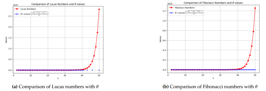
Mathematically, this behavior can be explained by examining the growth rates of Fibonacci and Lucas numbers. These sequences grow exponentially at a rate governed by the golden ratio \(\varphi\approx1.618\). As \(n\) increases, the individual terms \(F_{n+1}\), \(F_{n+2}\), \(F_{n+3}\), and \(F_n\) also grow exponentially, and the ratio between successive Fibonacci or Lucas numbers approaches \(\varphi\).
When calculating \(\theta\), the numerator \[\sqrt{F_{n+1}^2+F_{n+2}^2+F_{n+3}^2}\] and the denominator \(F_n\) both grow exponentially. Therefore, their quotient approaches a constant value. Consequently, the resulting \(\theta\) stabilizes, demonstrating a saturation effect.
This saturation can be interpreted as a form of convergence to a constant: despite the unbounded growth of Fibonacci and Lucas numbers, the relative growth between the terms becomes less significant as \(n\) becomes large. This suggests that, at large scales, the dynamic behavior of the sequences is increasingly governed by their limiting ratios, especially the golden ratio, while the effect of individual terms becomes less dominant.
Mathematical stability. The stabilization of the \(\theta\) values for large \(n\) indicates a form of mathematical stability. This can be useful in contexts where limiting or asymptotic behavior is of interest. It implies that although Fibonacci and Lucas numbers grow rapidly, their interactions, as represented by \(\theta\), tend toward a predictable and stable pattern.
Behavioral interpretation. From a conceptual point of view, the stabilization of \(\theta\) despite the growth of the sequence values suggests a limiting behavior inherent in recursive structures such as the Fibonacci and Lucas sequences. This provides insight into how recursive relations exhibit predictable long-term behavior, regardless of the magnitude of their individual terms.
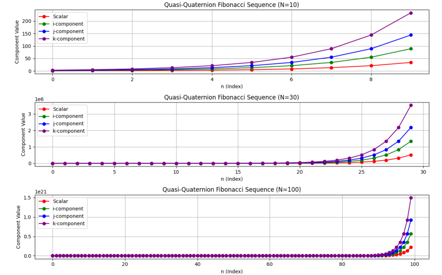
In Figure 3, for \(n=10\), the first few terms of the sequence are observed, reflecting the initial growth rate of the sequence. These first terms indicate that the sequence is sensitive to the initial conditions, with more pronounced changes in the early steps. Specifically, for \(n=10\), we observe sharp growth in the early terms of the sequence. The generating function is given by \[\sum_{n=0}^{\infty}QF_nx^n = \frac{QF_0+(QF_1-QF_0)x}{1-x-x^2},\] where \[QF_0=e_1+e_2+2e_3 \qquad \text{and} \qquad QF_1=1+e_1+2e_2+3e_3\] are the initial Fibonacci quasi-quaternion components.
In the graph, the scalar component grows more slowly compared with the vector components \(e_1\), \(e_2\), and \(e_3\), which increase more rapidly.
Slow growth of the scalar component. The initial values \(QF_0\) and \(QF_1\) result in a slower growth rate for the scalar component. This behavior can be attributed to the initial conditions, where the scalar component’s growth is less pronounced in the early stages of the sequence.
Rapid growth of the vector components. The vector components \(e_1\), \(e_2\), and \(e_3\) tend to grow more rapidly at the beginning because of the differences among the initial terms. This produces a sharper increase in these components when \(x\) is small.
For \(n=30\), the terms of the sequence exhibit a more balanced growth pattern. At this stage, the differences among the terms begin to level off, and the growth rates of the components become more consistent. The graph shows that as \(n\) increases, the terms begin to grow at a more uniform rate, with the scalar component also growing more significantly.
The recurrence relation for the sequence is \[QF_n=QF_{n-1}+QF_{n-2}.\] This recurrence relation implies that each term depends on the sum of the two previous terms, which leads to a more stable growth pattern as \(n\) increases.
Similarity among vector components. By \(n=30\), the growth rates of the vector components \(e_1\), \(e_2\), and \(e_3\) start to become more similar. This reflects the asymptotic convergence of the components’ growth rates. The influence of each term becomes more balanced, resulting in a more consistent increase in each component.
Stabilization of the scalar component. The scalar component continues to grow, but at a more stable rate, indicating that the sequence is approaching its asymptotic behavior. The growth of the scalar component stabilizes as earlier terms become less dominant.
Finally, for \(n=100\), the sequence approaches its asymptotic behavior, where the relative growth rates of the components reach a steady pattern. The graph for \(n=100\) shows that the terms exhibit more regular and stable growth, with differences among the components becoming less pronounced. As \(n\) increases, the relative growth behavior of the sequence stabilizes.
Mathematically, for large \(n\), the growth of the sequence can be approximated by \[QF_n\sim \lambda^n,\] where \(\lambda\) is a constant that determines the growth rate of the sequence. The growth of each term tends to stabilize at this rate, and the relative difference among components becomes negligible.
Asymptotic stability. At \(n=100\), the growth rates of the components stabilize, and each component grows according to a consistent rate. This reflects the expected asymptotic behavior of the sequence, where each term grows according to a fixed growth factor \(\lambda\).
Stabilization of the scalar component. The scalar component, while still growing, does so at a more stable relative rate. This indicates that the growth has approached an asymptotic pattern in which the influence of earlier terms becomes negligible.
In Figure 4, the \(x\)-axis represents the real component of the quasi-quaternion \(QF_n^k\), namely \(\cos(k\theta)\), while the \(y\)-axis represents the imaginary component, namely \(\vec{t}\sin(k\theta)\).
For \(n=10\), Figure 4 shows that, for smaller values of \(n\), the Fibonacci numbers grow relatively slowly, leading to more defined and less extreme vector magnitudes. The vectors \[QF_n^k=\cos(k\theta)+\vec{t}\sin(k\theta)\] exhibit stable directions as \(k\) increases, showing a clear pattern in the behavior of the quasi-quaternion with small variations in magnitude and direction.
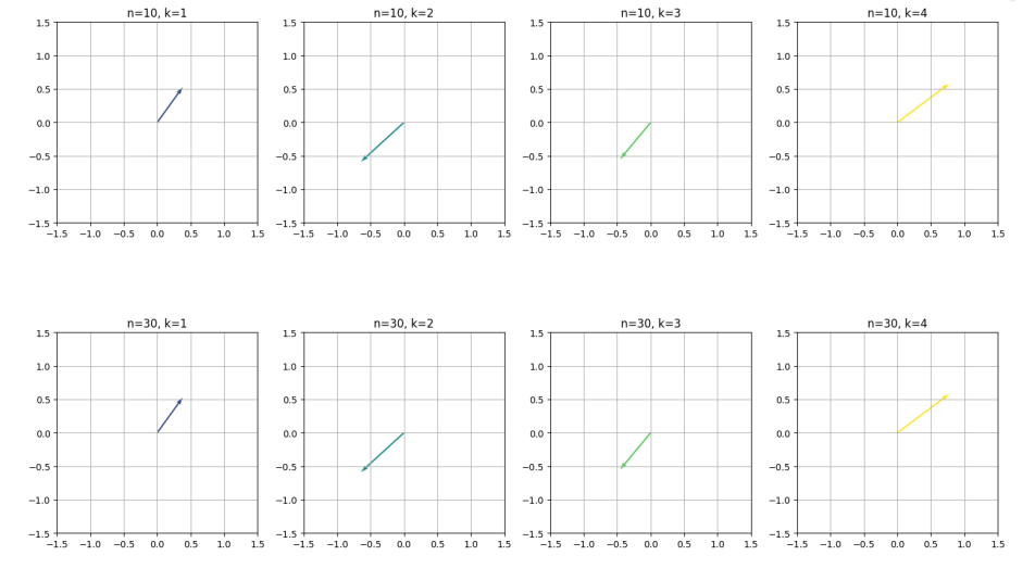
For \(n=30\), as \(n\) increases, the Fibonacci numbers become much larger, leading to a more pronounced effect on the angle \(\theta\), which influences the magnitude and direction of the quasi-quaternion. The vectors corresponding to higher values of \(k\) may appear more compressed or stretched along certain axes, reflecting the growth of the Fibonacci sequence and the effect of De Moivre’s formula on the powers of the quasi-quaternion.
The vectors for higher powers \(k\) move in more consistent patterns, demonstrating the influence of the Fibonacci growth rate on the quasi-quaternion structure. Larger values of \(n\) lead to greater angular shifts, affecting the representation of \(QF_n^k\) in the plot. In conclusion, the plots show how the quasi-quaternion evolves as \(n\) and \(k\) vary, with \(n=10\) showing smoother and smaller changes, while \(n=30\) shows more complex behavior due to the larger Fibonacci numbers.
In this study, we introduced Fibonacci and Lucas quasi-quaternions and investigated their algebraic and number-theoretic properties within the framework of quasi-quaternion algebra. We established fundamental results, including recurrence relations, Binet-type formulas, generating functions, and sum formulas. In addition, several classical identities, such as the Cassini, Catalan, d’Ocagne, Vajda, and Honsberger identities, were extended to the quasi-quaternion setting.
Furthermore, we presented matrix representations of Fibonacci and Lucas quasi-quaternions and derived explicit expressions for the powers of the associated matrices. We also examined De Moivre-type formulas in this framework, providing a structured approach to understanding powers of these elements.
The graphical representations included in the paper serve as visual illustrations of the theoretical results. In particular, they highlight the growth behavior and component-wise structure of the quasi-quaternion sequences. These figures are intended to support intuition and complement the analytical results rather than to suggest direct practical applications.
Overall, the results contribute to a deeper understanding of how classical number sequences can be embedded into quasi-quaternion algebra and how their structural properties extend in this setting. Future work may explore further algebraic generalizations and related theoretical developments.