
Let \(\Omega=[0,1]\times[0,1]\subset \mathbb{R}^{2}\). Consider first the incompressible time-independent Navier–Stokes system \[\label{eq145} \left\{ \begin{array}{ll} \nu \nabla^2u-u u_x-vu_y-P_x=0, & \\[1mm] \nu \nabla^2v-u v_x-vv_y-P_y=0, & \\[1mm] u_x+v_y=0, & \text{in }\Omega. \end{array} \right. \tag{1}\] Here, \(\nu>0\) is a small constant to be specified, and \(\mathbf{u}=(u,v,P)\in W^{1,2}(\Omega;\mathbb{R}^{3}),\) where \(u\) denotes the fluid velocity in the direction \(\mathbf{i}=(1,0)\in\mathbb{R}^{2},\) \(v\) denotes the fluid velocity in the direction \(\mathbf{j}=(0,1)\in\mathbb{R}^{2},\) and \(P\) is the corresponding pressure field. The boundary conditions are prescribed as follows: \[\label{bc-original} \left\{ \begin{aligned} u(0,y)&=\hat{u}_0(y), & v(0,y)&=0, & P(0,y)&=\hat{P}_0(y), && 0\leq y\leq 1,\\ u(x,0)&=0, & v(x,0)&=0, & P_y(x,0)&=0, && 0\leq x\leq 1,\\ u(x,1)&=0, & v(x,1)&=0, & P_y(x,1)&=0, && 0\leq x\leq 1,\\ u_x(1,y)&=0, & v_x(1,y)&=0, & P(1,y)&=\hat{P}_1(y), && 0\leq y\leq 1. \end{aligned} \right. \tag{2}\]
Proceeding as in [1], observe that from Eq. (1), we have \[\begin{aligned} \label{eq112} \frac{\partial}{\partial x} \left( \nu \nabla^2u-u u_x-vu_y-P_x \right) + \frac{\partial}{\partial y} \left( \nu \nabla^2v-u v_x-vv_y-P_y \right) =0. \end{aligned} \tag{3}\] Thus, \[\begin{aligned} \label{eq148} \nu \nabla^2(u_x+v_y) =&\, \nabla^2P+u_x^2+v_y^2+2u_yv_x +u(u_x+v_y)_x+v(u_x+v_y)_y. \end{aligned} \tag{4}\] Therefore, assuming \[\nabla^2P+u_x^2+v_y^2+2u_yv_x=0, \qquad \text{in }\Omega,\] we obtain \[\label{eq1510} \nu \nabla^2(u_x+v_y) = u(u_x+v_y)_x+v(u_x+v_y)_y. \tag{5}\]
We also suppose that \(\nu\), \(u\), and \(v\) are such that \[w=0,\qquad \text{in }\Omega,\] with the boundary condition \[w=0,\qquad \text{on }\partial\Omega,\] is the unique solution of the equation \[\nu\nabla^2w-uw_x-vw_y=0, \qquad \text{in }\Omega.\] Hence, from this and (5), we obtain \[u_x+v_y=w=0, \qquad \text{in }\Omega,\] and \[u_x+v_y=w=0, \qquad \text{on }\partial\Omega.\]
Remark 1. In such a case, we must drop the boundary conditions in \(P\). Indeed, from the results indicated above, we obtain the following resulting system: \[\label{eq159a} \left\{ \begin{array}{ll} \nu \nabla^2u-u u_x-vu_y-P_x=0, & \\[1mm] \nu \nabla^2v-u v_x-vv_y-P_y=0, & \\[1mm] \nabla^2P+u_x^2+v_y^2+2u_yv_x=0, & \text{in }\Omega, \end{array} \right. \tag{6}\] with the boundary conditions \[\label{bc-reduced} \left\{ \begin{aligned} u(0,y)&=\hat{u}_0(y), & v(0,y)&=0, && 0\leq y\leq 1,\\ u(x,0)&=0, & v(x,0)&=0, && 0\leq x\leq 1,\\ u(x,1)&=0, & v(x,1)&=0, && 0\leq x\leq 1,\\ u_x(1,y)&=0, & v_x(1,y)&=0, && 0\leq y\leq 1,\\ u_x+v_y&=0, &&& \text{on }\partial\Omega. \end{aligned} \right. \tag{7}\]
Remark 2. We understand that the procedure for obtaining this last elliptic system is very well known in numerical fluid mechanics. In my view, our only original contribution was to obtain the correct boundary condition \[u_x+v_y=0, \qquad \text{on }\partial\Omega,\] as indicated in [1].
Considering this context, we solve the following approximate Navier–Stokes system: \[\label{eq159} \left\{ \begin{array}{ll} \nu \nabla^2u-u u_x-vu_y-P_x=0, & \\[1mm] \nu \nabla^2v-u v_x-vv_y-P_y=0, & \\[1mm] \nabla^2P+u_x^2+v_y^2+2u_yv_x=0, & \text{in }\Omega, \end{array} \right. \tag{8}\] with the boundary conditions \[\label{bc-approx} \left\{ \begin{aligned} u(0,y)&=\hat{u}_0(y), & v(0,y)&=0, & P(0,y)&=\hat{P}_0(y), && 0\leq y\leq 1,\\ u(x,0)&=0, & v(x,0)&=0, & P_y(x,0)&=0, && 0\leq x\leq 1,\\ u(x,1)&=0, & v(x,1)&=0, & P_y(x,1)&=0, && 0\leq x\leq 1,\\ u_x(1,y)&=0, & v_x(1,y)&=0, & P(1,y)&=\hat{P}_1(y), && 0\leq y\leq 1. \end{aligned} \right. \tag{9}\]
Regarding the references, first we recall that the generalized method of lines was originally introduced in the book [2] in 2011. It is worth highlighting that standard models in fluid mechanics are addressed in [3, 4]. Related results may be found in [5– 8]. For related numerical approaches and results, we cite [1, 9– 11]. Other more general and related results may be found in [12– 4]. For the Sobolev spaces involved, we cite [15].
Intending to apply the generalized method of lines approach in a Cartesian-coordinate context, we discretize the domain \(\Omega\) in the \(x\) direction by defining \[d=\frac{1}{m_8},\] where \(m_8=800\) and \(m_8\) is the number of vertical straight lines.
Observe that, similarly to what is found in the references [2, 13, 14], already considering an initial solution \[\{(u_0)_n,(v_0)_n,(P_0)_n\}=U_0,\] fixing \(U_1=U_0\), and considering a proximal formulation through an appropriate constant \(K>0\), we may obtain the last equation in partial finite differences. Standard finite-difference schemes may be found in [11]. Thus, we have \[\begin{aligned} \label{eq1801} \nu& \left( \frac{u_{n+1}-2u_n+u_{n-1}}{d^2} + \frac{m_2u_n}{d_1^2} \right) -(u_0)_n \frac{(u_0)_n-(u_0)_{n-1}}{d} -(v_0)_n \frac{m_1}{d_1}(u_0)_n \nonumber\\ &\quad -K(u_n-(u_0)_n) -\frac{(P_0)_n-(P_0)_{n-1}}{d} =0, \end{aligned} \tag{10}\] \[\begin{aligned} \label{eq1802} \nu& \left( \frac{v_{n+1}-2v_n+v_{n-1}}{d^2} + \frac{m_2v_n}{d_1^2} \right) -(u_0)_n \frac{(v_0)_n-(v_0)_{n-1}}{d} -(v_0)_n \frac{m_1}{d_1}(v_0)_n \nonumber\\ &\quad -K(v_n-(v_0)_n) -\frac{m_1(P_0)_n}{d_1} =0, \end{aligned} \tag{11}\] and \[\begin{aligned} \label{eq1803} & \left( \frac{P_{n+1}-2P_n+P_{n-1}}{d^2} + \frac{m_{22}P_n}{d_1^2} \right) -K(P_n-(P_0)_n) + \frac{(u_0)_n-(u_0)_{n-1}}{d} \frac{(u_0)_n-(u_0)_{n-1}}{d} \nonumber\\ &\qquad + \frac{m_1(v_0)_n}{d_1} \frac{m_1(v_0)_n}{d_1} + 2 \frac{m_1(u_0)_n}{d_1} \frac{(v_0)_n-(v_0)_{n-1}}{d} =0, \end{aligned} \tag{12}\] for all \(n\in\{1,\ldots,m_8-1\}.\) Here, \(m_2\) is an appropriate matrix such that \(\frac{\partial^2u_n}{\partial y^2} \approx \frac{m_2u_n}{(d_1)_n^2}.\) That is, \[m_2 = \left[ \begin{array}{cccccc} -2 & 1 & 0 & 0 & \cdots & 0 \\ 1 & -2 & 1 & 0 & \cdots & 0 \\ \vdots & \vdots & \vdots & \vdots & \ddots & \vdots \\ 0 & 0 & 0 & \cdots & 1 & -2 \end{array} \right]_{(m_9-1)\times(m_9-1)}. \tag{13}\] Moreover, \[m_{22} = \left[ \begin{array}{cccccc} -1 & 1 & 0 & 0 & \cdots & 0 \\ 1 & -2 & 1 & 0 & \cdots & 0 \\ \vdots & \vdots & \vdots & \vdots & \ddots & \vdots \\ 0 & 0 & 0 & \cdots & 1 & -1 \end{array} \right]_{(m_9-1)\times(m_9-1)}, \tag{14}\] \[m_{1a} = \left[ \begin{array}{cccccc} -1 & 1 & 0 & 0 & \cdots & 0 \\ 0 & -1 & 1 & 0 & \cdots & 0 \\ \vdots & \vdots & \vdots & \vdots & \ddots & \vdots \\ 0 & 0 & 0 & \cdots & 0 & -1 \end{array} \right]_{(m_9-1)\times(m_9-1)}, \tag{15}\] \[m_{1b} = \left[ \begin{array}{cccccc} 1 & 0 & 0 & 0 & \cdots & 0 \\ -1 & 1 & 0 & 0 & \cdots & 0 \\ \vdots & \vdots & \vdots & \vdots & \ddots & \vdots \\ 0 & 0 & 0 & \cdots & -1 & 1 \end{array} \right]_{(m_9-1)\times(m_9-1)}. \tag{16}\] Furthermore, \[m_1=\frac{m_{1a}+m_{1b}}{2}.\]
Here, \(m_9=120\), and \(d_1=\frac{1}{m_9}.\) Denoting \[\begin{aligned} (y_1)_n =& -(u_0)_n \frac{(u_0)_n-(u_0)_{n-1}}{d} -(v_0)_n \frac{m_1}{d_1}(u_0)_n +K(u_0)_n -\frac{(P_0)_n-(P_0)_{n-1}}{d}, \end{aligned} \tag{17}\] from (10), in particular for \(n=1\), we obtain \[\begin{aligned} \label{eq1804} \nu \left( \frac{u_{n+1}-2u_n+u_{n-1}}{d^2} + \frac{m_2u_n}{d_1^2} \right) -Ku_n+(y_1)_1 =0. \end{aligned} \tag{18}\] Thus, \[u_2-2u_1+\hat{u}_0 + \frac{m_2u_1}{(d_1)_1^2}d^2 + (y_1)_1\frac{d^2}{\nu} =0,\] so that \[u_1=m_{50}(1)u_2+z_1(1),\] where \[m_{50}(1) = \left( 2I_d – \frac{m_2d^2}{(d_1)_1^2} + K\frac{d^2}{\nu} \right)^{-1},\] and \[z_1(1) = m_{50}(1) \left( \hat{u}_0+(y_1)_1\frac{d^2}{\nu} \right).\]
Reasoning inductively, having \[u_{n-1}=m_{50}(n-1)u_n+z_1(n-1),\] we obtain \[u_{n+1}-2u_n + m_{50}(n-1)u_n + z_1(n-1) + \frac{m_2u_n}{(d_1)_n^2}d^2 + (y_1)_n\frac{d^2}{\nu} =0.\] Therefore, \[u_n=m_{50}(n)u_{n+1}+z_1(n),\] where \[m_{50}(n) = \left( 2I_d – \frac{m_2d^2}{(d_1)_n^2} + K\frac{d^2}{\nu} – m_{50}(n-1) \right)^{-1},\] and \[z_1(n) = m_{50}(n) \left( (y_1)_n\frac{d^2}{\nu} + z_1(n-1) \right).\]
The induction is complete.
Observe that from the boundary condition \(u_x(1,y)=0,\) we have \(u_{m_8}=u_{m_8-1}.\) Thus, \[u_{m_8-1} = u_{m_8} = m_{50}(m_8-1)u_{m_8}+z_1(m_8-1).\] Consequently, \[u_{m_8} = \left(I_d-m_{50}(m_8-1)\right)^{-1}z_1(m_8-1),\] and \[u_{m_8-1}=u_{m_8}.\]
Similarly, we obtain \[u_{m_8-2} = m_{50}(m_8-2)u_{m_8-1}+z_1(m_8-2),\] and so on, up to finding \[u_1=m_{50}(1)u_2+z_1(1).\]
The next step is to replace \(\{(u_0)_n\}\) by \(\{u_n\}\) and repeat this procedure until an appropriate convergence criterion is satisfied. Similarly, we may obtain \(\{v_n\}\) and \(\{P_n\}\).
Denoting \(U=\{u_n,v_n,P_n\},\) we evaluate \[\label{eq19900} \|U_1-U\|. \tag{19}\]
The next step is to replace \(U_1\) by \(U=\{u_n,v_n,P_n\}.\) Thus, we keep repeating the whole process until \(\|U_1-U\|\rightarrow 0\) in Eq. (19). The problem is then solved.
Consider again the approximate Navier–Stokes system \[\label{eq159-conv} \left\{ \begin{array}{ll} \nu \nabla^2u-u u_x-vu_y-P_x=0, & \\[1mm] \nu \nabla^2v-u v_x-vv_y-P_y=0, & \\[1mm] \nabla^2P+u_x^2+v_y^2+2u_yv_x=0, & \text{in }\Omega, \end{array} \right. \tag{20}\] with the previously indicated boundary conditions, namely \[\label{bc-conv} \left\{ \begin{aligned} u(0,y)&=\hat{u}_0(y), & v(0,y)&=0, & P(0,y)&=\hat{P}_0(y), && 0\leq y\leq 1,\\ u(x,0)&=0, & v(x,0)&=0, & P_y(x,0)&=0, && 0\leq x\leq 1,\\ u(x,1)&=0, & v(x,1)&=0, & P_y(x,1)&=0, && 0\leq x\leq 1,\\ u_x(1,y)&=0, & v_x(1,y)&=0, & P(1,y)&=\hat{P}_1(y), && 0\leq y\leq 1. \end{aligned} \right. \tag{21}\]
Denoting \[\nabla^2u_k = \left\{ \frac{(u_k)_{i,j+1}-2(u_k)_{i,j}+(u_k)_{i,j-1}}{d^2} + \frac{(m_2)_{il}(u_k)_{lj}}{d_1^2} \right\}, \] and including a proximal term through a constant \(K>0\), in a finite-difference context, the first equation in the last system becomes \[\begin{aligned} &\nu \nabla^2u_{k+1} -(u_k)_{i,j} \left( \frac{(u_k)_{i,j+1}-(u_k)_{i,j}}{d} \right) -(v_k)_{i,j} \left( \frac{(m_1)_{il}(u_k)_{l,j}}{d_1} \right) \nonumber\\ &\qquad -\frac{(P_k)_{i,j+1}-(P_k)_{i,j}}{d} -K(u_{k+1}-u_k) =0. \end{aligned} \tag{22}\]
Denoting \[\begin{aligned} H_1(u_k,v_k,P_k) =&\, Ku_k – \left\{ (u_k)_{i,j} \left( \frac{(u_k)_{i,j+1}-(u_k)_{i,j}}{d} \right) \right\} \nonumber\\ &- \left\{ (v_k)_{i,j} \left( \frac{(m_1)_{il}(u_k)_{l,j}}{d_1} \right) \right\} – \left\{ \frac{(P_k)_{i,j+1}-(P_k)_{i,j}}{d} \right\}, \end{aligned} \tag{23}\] we obtain \[\nu \nabla^2u_{k+1}-Ku_{k+1}+H_1(u_k,v_k,P_k)=0.\] From this last linear equation, we may obtain \[u_{k+1}=F_1(u_k,v_k,P_k)=u_{k+1}(u_k,v_k,P_k).\]
Considering the algorithm that we have utilized, we set the following second equation in finite differences: \[\begin{aligned} &\nu \nabla^2v_{k+1} -(u_{k+1})_{i,j} \left( \frac{(v_k)_{i,j+1}-(v_k)_{i,j}}{d} \right) -(v_k)_{i,j} \left( \frac{(m_1)_{il}(v_k)_{l,j}}{d_1} \right) \nonumber\\ &\qquad -\frac{(m_1)_{il}P_{lj}}{d_1} -K(v_{k+1}-v_k) =0. \end{aligned} \tag{24}\] Similarly to the previous equation, considering that \[u_{k+1}=F_1(u_k,v_k,P_k)=u_{k+1}(u_k,v_k,P_k),\] we obtain \[\nu \nabla^2v_{k+1}-Kv_{k+1}+H_2(u_k,v_k,P_k)=0,\] for an appropriate matrix \(H_2\), so that \[v_{k+1}=F_2(u_k,v_k,P_k)=v_{k+1}(u_k,v_k,P_k).\]
Finally, for the third equation, we may also obtain \[\nabla^2P_{k+1}-KP_{k+1}+H_3(u_k,v_k,P_k)=0.\]
Denoting \(\mathbf{u}_k=(u_k,v_k,P_k),\) we have obtained \[\label{eq159C} \left[ \begin{array}{ccc} -\nu \nabla^2+KI_d & 0 & 0\\[1mm] 0 & -\nu \nabla^2+KI_d & 0\\[1mm] 0 & 0 & -\nabla^2+KI_d \end{array} \right] \mathbf{u}_{k+1} = \left[ \begin{array}{c} H_1(\mathbf{u}_k)\\[1mm] H_2(\mathbf{u}_k)\\[1mm] H_3(\mathbf{u}_k) \end{array} \right]. \tag{25}\]
Thus, \[\begin{aligned} \label{eq159B} & \left[ \begin{array}{ccc} -\nu \nabla^2+KI_d & 0 & 0\\[1mm] 0 & -\nu \nabla^2+KI_d & 0\\[1mm] 0 & 0 & -\nabla^2+KI_d \end{array} \right] (\mathbf{u}_{k+2}-\mathbf{u}_{k+1}) = \left[ \begin{array}{c} H_1(\mathbf{u}_{k+1})-H_1(\mathbf{u}_k)\\[1mm] H_2(\mathbf{u}_{k+1})-H_2(\mathbf{u}_k)\\[1mm] H_3(\mathbf{u}_{k+1})-H_3(\mathbf{u}_k) \end{array} \right]. \end{aligned} \tag{26}\] Hence, there exists a symmetric matrix \(M(\mathbf{u}_k,\mathbf{u}_{k+1})\) such that \[\begin{aligned} \label{eq159A} & \left[ \begin{array}{ccc} -\nu \nabla^2+KI_d & 0 & 0\\[1mm] 0 & -\nu \nabla^2+KI_d & 0\\[1mm] 0 & 0 & -\nabla^2+KI_d \end{array} \right] (\mathbf{u}_{k+2}-\mathbf{u}_{k+1}) = M(\mathbf{u}_k,\mathbf{u}_{k+1})(\mathbf{u}_{k+1}-\mathbf{u}_k). \end{aligned} \tag{27}\]
Denoting \[\begin{aligned} \label{eq159A1} L_\nu = \left[ \begin{array}{ccc} -\nu \nabla^2+KI_d & 0 & 0\\[1mm] 0 & -\nu \nabla^2+KI_d & 0\\[1mm] 0 & 0 & -\nabla^2+KI_d \end{array} \right], \end{aligned} \tag{28}\] we have \(\mathbf{u}_{k+1} = L_\nu^{-1}\{H_j(\mathbf{u}_k)\}_{3\times 1} \equiv \mathbf{F}(\mathbf{u}_k).\) Here, we assume that \(\hat{\mathbf{u}}_0=(\hat{u}_0,\hat{v}_0,\hat{P}_0)\) and \(0<\alpha_1<1\) are such that there exists \(r>0\) satisfying \[\alpha_1L_\nu \geq M(\mathbf{u},\mathbf{v}) \geq \mathbf{0}, \qquad \forall\,\mathbf{u},\mathbf{v}\in B_r(\hat{\mathbf{u}}_0).\] Observe that \[\left\|L_\nu^{-1}M(\mathbf{u},\mathbf{v})\right\| \leq \alpha_1<1, \qquad \forall\,\mathbf{u},\mathbf{v}\in B_r(\hat{\mathbf{u}}_0).\]
Observe also that \[\mathbf{u}_{k+2}-\mathbf{u}_{k+1} = L_\nu^{-1} M(\mathbf{u}_k,\mathbf{u}_{k+1}) (\mathbf{u}_{k+1}-\mathbf{u}_k).\] Define \(r_1=(1-\alpha_1)r.\) Assume that \(K>0\) is large enough so that \(\mathbf{u}_1=\mathbf{F}(\hat{\mathbf{u}}_0)\) also satisfies \(\|\mathbf{u}_1-\hat{\mathbf{u}}_0\|<r_1<r,\) and therefore \(\mathbf{u}_1\in B_r(\hat{\mathbf{u}}_0).\)
Thus, from this result and from \(\mathbf{u}_2-\mathbf{u}_1 = L_\nu^{-1} M(\hat{\mathbf{u}}_0,\mathbf{u}_1) (\mathbf{u}_1-\hat{\mathbf{u}}_0),\) we obtain \[\begin{aligned} \|\mathbf{u}_2-\mathbf{u}_1\| &= \left\| L_\nu^{-1} M(\hat{\mathbf{u}}_0,\mathbf{u}_1) \right\| \, \|\mathbf{u}_1-\hat{\mathbf{u}}_0\| \leq \alpha_1\|\mathbf{u}_1-\hat{\mathbf{u}}_0\| \leq \alpha_1r_1. \end{aligned} \tag{29}\]
Reasoning inductively, for \(k\geq 1\), assume now that \[\mathbf{u}_j\in B_r(\hat{\mathbf{u}}_0), \qquad \forall\,j\in\{1,\ldots,k+1\}.\] In such a case, we have \[\|\mathbf{u}_2-\mathbf{u}_1\| \leq \alpha_1r_1,\] \[\|\mathbf{u}_3-\mathbf{u}_2\| \leq \alpha_1\|\mathbf{u}_2-\mathbf{u}_1\| \leq \alpha_1^2r_1,\] and so on, up to obtaining \[\|\mathbf{u}_{k+2}-\mathbf{u}_{k+1}\| \leq \alpha_1^{k+1}r_1.\]
Thus, \[\begin{aligned} \|\mathbf{u}_{k+2}-\hat{\mathbf{u}}_0\| =&\, \|\mathbf{u}_{k+2}-\mathbf{u}_{k+1} +\mathbf{u}_{k+1}-\cdots-\mathbf{u}_2-\mathbf{u}_1 +\mathbf{u}_1-\hat{\mathbf{u}}_0\| \nonumber\\ \leq&\, \|\mathbf{u}_{k+2}-\mathbf{u}_{k+1}\| + \|\mathbf{u}_{k+1}-\mathbf{u}_k\| +\cdots + \|\mathbf{u}_1-\hat{\mathbf{u}}_0\| \nonumber\\ \leq&\, \alpha_1^{k+1}r_1 + \alpha_1^kr_1 + \cdots + \alpha_1r_1 + r_1 \nonumber\\ <&\, \sum_{j=0}^{\infty}\alpha_1^j r_1 \nonumber\\ =&\, \frac{r_1}{1-\alpha_1} \nonumber\\ =&\, r. \end{aligned} \tag{30}\] Therefore, \[\mathbf{u}_{k+2}\in B_r(\hat{\mathbf{u}}_0).\]
The induction is complete, so that \[\mathbf{u}_k\in B_r(\hat{\mathbf{u}}_0), \qquad \forall\,k\in\mathbb{N}.\]
From these results, we may infer that \[\begin{aligned} \|\mathbf{u}_{k+2}-\mathbf{u}_{k+1}\| &\leq \left\| L_\nu^{-1} M(\mathbf{u}_k,\mathbf{u}_{k+1}) \right\| \, \|\mathbf{u}_{k+1}-\mathbf{u}_k\| \nonumber\\ &\leq \alpha_1 \|\mathbf{u}_{k+1}-\mathbf{u}_k\|, \qquad \forall\,k\in\mathbb{N}. \end{aligned} \tag{31}\]
Consequently, from the Banach fixed point theorem, there exists \(\mathbf{u}_0\in\overline{B_r(\hat{\mathbf{u}}_0)}\) such that \(\mathbf{u}_k\rightarrow \mathbf{u}_0.\) Finally, from this last result, by continuity, we obtain \(\lim_{k\rightarrow\infty}\mathbf{u}_{k+1} = \mathbf{u}_0 = \lim_{k\rightarrow\infty}\mathbf{F}(\mathbf{u}_k) = \mathbf{F}(\mathbf{u}_0).\) In summary, the vector \(\mathbf{u}_0\) solves the approximate Navier–Stokes system in question in a finite-difference context. The objective of this section is complete.
In this section, again for \(\Omega=[0,1]\times[0,1],\) we solve the following time-dependent approximate Navier–Stokes system:
\[\label{eq159-time} \left\{ \begin{array}{ll} u_t=\nu \nabla^2u-u u_x-vu_y-P_x, & \\[1mm] v_t=\nu \nabla^2v-u v_x-vv_y-P_y, & \\[1mm] \nabla^2P+u_x^2+v_y^2+2u_yv_x=0, & \text{in }\Omega\times[0,T]. \end{array} \right. \tag{32}\] The boundary conditions are prescribed as follows: \[\label{bc-time} \left\{ \begin{aligned} u(0,y,t)&=\hat{u}_0(y), & v(0,y,t)&=0, & P(0,y,t)&=\hat{P}_0(y), && (y,t)\in[0,1]\times[0,T],\\ u(x,0,t)&=0, & v(x,0,t)&=0, & P_y(x,0,t)&=0, && (x,t)\in[0,1]\times[0,T],\\ u(x,1,t)&=0, & v(x,1,t)&=0, & P_y(x,1,t)&=0, && (x,t)\in[0,1]\times[0,T],\\ u_x(1,y,t)&=0, & v_x(1,y,t)&=0, & P(1,y,t)&=\hat{P}_1(y), && (y,t)\in[0,1]\times[0,T]. \end{aligned} \right. \tag{33}\] The initial condition is given by \[(u(x,y,0),v(x,y,0)) = (u_0^*(x,y),v_0^*(x,y)).\]
Intending to apply the generalized method of lines approach in a Cartesian-coordinate context, we discretize the domain \(\Omega\) in the \(x\) direction by defining \(d=\frac{1}{m_8},\) where \(m_8=800\) and \(m_8\) is the number of vertical straight lines. We also set \(T=1,\) and discretize time by taking \(m_{10}=300, \quad d_2=\frac{1}{m_{10}}.\) For \(k=2\), already considering an initial solution \(\{u_n^1,v_n^1\} = \{(u_0)_n^*,(v_0)_n^*\},\) with the corresponding \(\{(P_0)_n^*\}\) obtained from the solution of the time-independent case for \(\nu=0.55\), and setting \(\{(u_0)_n^k,(v_0)_n^k,(P_0)_n^k\} = \{(u_0)_n^*,(v_0)_n^*,(P_0)_n^*\},\) similarly to the time-independent case, we may obtain \(\{u_n^k,v_n^k,P_n^k\},\) through the following system of finite-difference equations: \[\begin{aligned} \label{eq1805} & -\frac{u_n^k-u_n^{k-1}}{d_2} + \nu \left( \frac{u_{n+1}^k-2u_n^k+u_{n-1}^k}{d^2} + \frac{m_2u_n^k}{d_1^2} \right) -(u_0)_n^k \frac{(u_0)_n^k-(u_0)_{n-1}^k}{d} \nonumber\\ &\qquad -(v_0)_n^k \frac{m_1}{d_1}(u_0)_n^k – \frac{(P_0)_n^k-(P_0)_{n-1}^k}{d} =0, \end{aligned} \tag{34}\] \[\begin{aligned} \label{eq1806} & -\frac{v_n^k-v_n^{k-1}}{d_2} + \nu \left( \frac{v_{n+1}^k-2v_n^k+v_{n-1}^k}{d^2} + \frac{m_2v_n^k}{d_1^2} \right) -(u_0)_n^k \frac{(v_0)_n^k-(v_0)_{n-1}^k}{d} \nonumber\\ &\qquad -(v_0)_n^k \frac{m_1}{d_1}(v_0)_n^k – \frac{m_1(P_0)_n^k}{d_1} =0, \end{aligned} \tag{35}\] and \[\begin{aligned} \label{eq1807} & \left( \frac{P_{n+1}^k-2P_n^k+P_{n-1}^k}{d^2} + \frac{m_{22}P_n^k}{d_1^2} \right) – K(P_n^k-(P_0)_n^k) + \frac{(u_0)_n^k-(u_0)_{n-1}^k}{d} \frac{(u_0)_n^k-(u_0)_{n-1}^k}{d} \nonumber\\ &\qquad + \frac{m_1(v_0)_n^k}{d_1} \frac{m_1(v_0)_n^k}{d_1} + 2 \frac{m_1(u_0)_n^k}{d_1} \frac{(v_0)_n^k-(v_0)_{n-1}^k}{d} =0, \end{aligned} \tag{36}\] for all \(n\in\{1,\ldots,m_8-1\} \quad \text{and} \quad k=2.\)
The next step is to replace \(\{(u_0)_n^k,(v_0)_n^k,(P_0)_n^k\}\) by \(\{u_n^k,v_n^k,P_n^k\},\) and then repeat this procedure until an appropriate convergence criterion is satisfied. Reasoning inductively, for \(2<k<m_{10},\) having \(\{u_n^{k-1},v_n^{k-1},P_n^{k-1}\},\) with the starting solution \(\{(u_0)_n^k,(v_0)_n^k,(P_0)_n^k\} = \{u_n^{k-1},v_n^{k-1},P_n^{k-1}\},\) similarly, we may obtain \(\{u_n^k,v_n^k,P_n^k\}.\) The induction on \(k\) is complete. The problem is then solved.
As previously mentioned, the numerical results were obtained for \[m_8=800 \qquad \text{and} \qquad m_9=120.\]
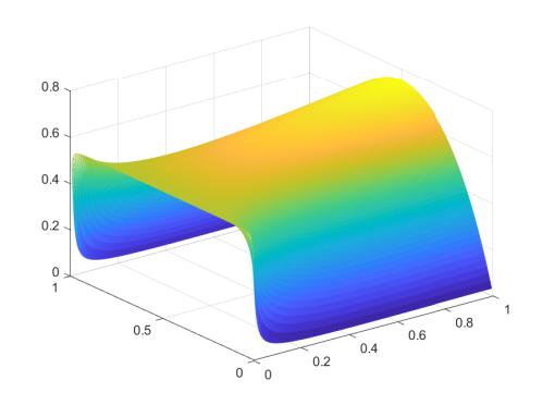
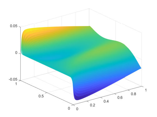
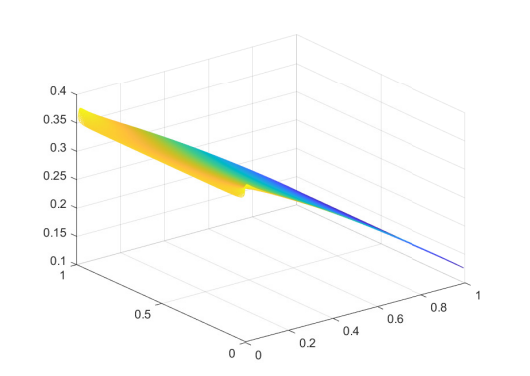
For the time-independent case, we set \[\nu=0.03,\qquad \hat{u}_0\equiv 0.55,\qquad \hat{P}_0=0.35,\qquad \hat{P}_1=0.125, \qquad \text{in }[0,1].\] The units refer to the International System of Units, with a standard normalization commonly used in fluid mechanics.
For the obtained solutions \(u\), \(v\), and \(P\), see Figures 1, 2, and 3, respectively.
Concerning the last section and the corresponding algorithm, we emphasize that the solution of the last approximate Navier–Stokes system, including boundary conditions for the pressure field, may be such that \(\|u_x+v_y\|_{\infty}\) is large. In such a case, the continuity equation is not properly approximately solved throughout the domain, especially close to its boundaries. In order to address such issues, we propose another algorithm, which is described in the following lines. We solve the following Navier–Stokes system with no boundary conditions imposed on the pressure field: \[\label{eq159-second-algorithm} \left\{ \begin{array}{ll} \nu \nabla^2u-u u_x-vu_y-P_x=0, & \\[1mm] \nu \nabla^2v-u v_x-vv_y-P_y=0, & \\[1mm] u_x+v_y=0, & \text{in }\Omega, \end{array} \right. \tag{37}\] with the following boundary conditions: \[\label{bc-second-algorithm} \left\{ \begin{aligned} u(0,y)&=\hat{u}_0(y), & v(0,y)&=0, && 0\leq y\leq 1,\\ u(x,0)&=0, & v(x,0)&=0, && 0\leq x\leq 1,\\ u(x,1)&=0, & v(x,1)&=0, && 0\leq x\leq 1,\\ u_x(1,y)&=0, & v_x(1,y)&=0, && 0\leq y\leq 1. \end{aligned} \right. \tag{38}\]
Considering these boundary conditions, let \(N\) denote the number of vertical lines, as well as the number of nodes in the \(x\) and \(y\) directions, and define \[d=\frac{1}{N}.\] The corresponding algorithm is as follows.
Set \(b_{12}=10^{-4}, \quad n_{\max}\in\mathbb{N}, \quad k=1.\)
Choose an initial solution \(\{(u_0)_n,(v_0)_n\}.\)
] Set \(P_0=\{(P_0)_n\}=\{x_n\},\) and update \(k=k+1.\)
Here, generically denoting \(\nabla^2u_n = \frac{u_{n+1}-2u_n+u_{n-1}}{d^2} + \frac{m_2}{d^2}u_n,\) calculate, through an appropriate MATLAB function, \(\{u_n,v_n\}=\{u_n(x),v_n(x)\},\) such that \[\begin{aligned} &\nu \nabla^2u_n -K(u_n-(u_0)_n) -(u_0)_n \frac{(u_0)_n-(u_0)_{n-1}}{d} \nonumber\\ &\qquad -(v_0)_n m_1\frac{(u_0)_n}{d} -\frac{x_n-x_{n-1}}{d} =\mathbf{0}, \qquad \forall n\in\{1,\ldots,N-1\}, \end{aligned} \tag{39}\] and \[\begin{aligned} &\nu \nabla^2v_n -K(v_n-(v_0)_n) -(u_0)_n \frac{(v_0)_n-(v_0)_{n-1}}{d} \nonumber\\ &\qquad -(v_0)_n m_1\frac{(v_0)_n}{d} -\frac{m_1x_n}{d} =\mathbf{0}, \qquad \forall n\in\{1,\ldots,N-1\}. \end{aligned} \tag{40}\]
Having \(\{u_n,v_n\}=\{u_n(x),v_n(x)\},\) calculate \(\hat{x}=\{\hat{x}_n\}\) such that \(J(\hat{x})=\inf_x J(x),\) where, in a finite-difference context, \(J(x)=\int_{\Omega}(u_x(x)+v_y(x))^2\,dx.\)
If \(\|\{u_n(\hat{x})-(u_0)_n\}\|_{\infty}<b_{12},\) or \(k>n_{\max},\) then stop. Otherwise, set \(\{(u_0)_n,(v_0)_n\}:=\{u_n(\hat{x}),v_n(\hat{x})\},\) and return to item 3.
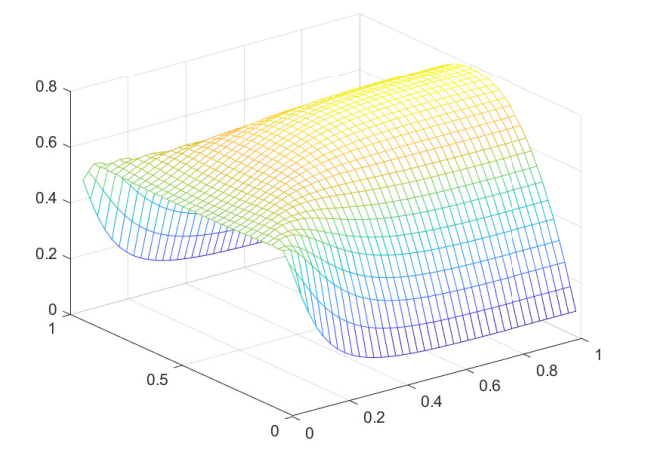
We developed a numerical example with \[\nu=0.15,\qquad \hat{u}_0\equiv 0.55,\qquad N=40,\qquad d=\frac{1}{N},\qquad d_1=\frac{1}{N}, \qquad K=250.\] For the graphs of the obtained solutions \(u\), \(v\), and \(P_0\), see Figures 4, 5, and 6, respectively.
Moreover, for the final solution, we also obtained \(\|u_x+v_y\|_{0,2} = \sqrt{\int_{\Omega}(u_x+v_y)^2\,dx} = 4.2608\times 10^{-8},\) and \(\|u_x+v_y\|_{\infty} = 1.2991\times 10^{-6}.\) Therefore, \(u_x+v_y\approx 0, \quad \text{in }\Omega,\) so that the continuity equation is approximately and satisfactorily solved, as expected.
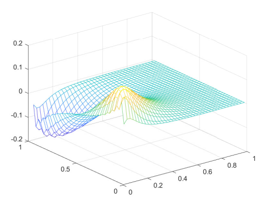
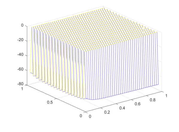
Remark 3. We have obtained negative values for the pressure field. However, this is not a relevant issue, since the pressure field is defined only up to an arbitrary constant \(C>0\), which may be added to \(P\) without producing any other changes in the system solution.
Finally, we obtained a highly oscillatory pressure field, suggesting that the convergence of the optimal \(P\) for the original infinite-dimensional model may occur only in a weak sense.
We now present the MATLAB implementation entitled
LinesNavierStokesMarch202610, through which the numerical
results reported above were obtained.
clear all

global u5 v5 P5 u1 uo vo Po m8 m9 S1 u v P W3 k10 e1 d d1

m8=40;

m9=40;

e1=0.15;

for i=1:m8

u1(:,i)=0.4*ones(m9-1,1);

end;

for i=1:m8

uo(:,i)=0.3*ones(m9-1,1);

vo(:,i)=0.1*ones(m9-1,1);

%Po(:,i)=0.3*ones(m9-1,1);

%u1(:,i)=0.3*ones(m9-1,1);

end;

k10=1;

b25=1;

xo(:,1)=ones((m8)*(m9-1),1);

%xo(:,1)=ones(28,1);

while (b25>10^(-4)) && (k10<49)

k10

k10=k10+1;

%X3=fminunc('funMarch20267A',xo);

X3=lsqnonlin('funMarch20267A',xo);

b25=max(max(abs(u1-uo)));

u1=uo;

xo=X3;

uo=u(:,:,1);

vo=v(:,:,1);

%Po=P(:,:,1);

uo(m9/2,m8/2)

end;

%u5=uo;

%v5=vo;

for i=1:m8

x1(i,1)=i*d;

end;

for j=1:m9-1

y1(j,1)=j*d1;

end;

mesh(x1,y1,u(:,:,1))
The auxiliary MATLAB function used in the implementation is entitled
funMarch20267A. It is given below.
function W5=funMarch20267A(x)

global u5 v5 P5 u1 uo vo Po m8 m9 S1 u v P W3 k10 e1 d d1

d=1/m8;

d1=1/m9;

e2=1.0;

%K=50;

K=250;

Id=eye(m9-1);

m2=zeros(m9-1,m9-1);

for i=2:m9-2

m2(i,i)=-2.0;

m2(i,i+1)=1.0;

m2(i,i-1)=1.0;

end;

m2(1,1)=-2.0;

m2(1,2)=1;

m2(m9-1,m9-1)=-2.0;

m2(m9-1,m9-2)=1.0;

m22=zeros(m9-1,m9-1);

for i=2:m9-2

m22(i,i)=-2.0;

m22(i,i+1)=1.0;

m22(i,i-1)=1.0;

end;

m22(1,1)=-1.0;

m22(1,2)=1;

m22(m9-1,m9-1)=-1.0;

m22(m9-1,m9-2)=1.0;

m1=zeros(m9-1,m9-1);

for i=2:m9-2

m1(i,i)=-1;

m1(i,i+1)=1;

end;

m1(1,1)=-1;

m1(1,2)=1;

m1(m9-1,m9-1)=-1;

m1a=zeros(m9-1,m9-1);

for i=2:m9-1

m1a(i,i)=1;

m1a(i,i-1)=-1;

end;

m1a(1,1)=1;

m3=m1;

m1=(m1+m1a)/2;


uoo(:,1)=.55*ones(m9-1,1);

voo(:,1)=0.0*ones(m9-1,1);

for i=1:m8-1

for j=1:m9-1

Po(j,i)=x(j+(i-1)*(m9-1),1);

end;

end;

for j=1:m9-1

Poo(j,1)=x(j+(m8-1)*(m9-1),1);

%Po(j,m8-1)=0.125;

end;


i=1;

m12=2*Id-m2/d1^2*d^2+K*d^2*Id/e1;

m50(:,:,i)=inv(m12);

z1(:,i)=m50(:,:,i)*(K*uo(:,i)*d^2/e1+uoo(:,1) ...
-(Po(:,i)-Poo(:,1))/d*d^2/e1 ...
-vo(:,i).*(m1*uo(:,i))/d1*d^2/e1 ...
-uo(:,i).*(uo(:,i)-uoo(:,1))/d*d^2/e1);


for i=2:m8-1

m12=2*Id-m2/d1^2*d^2-m50(:,:,i-1)+K*d^2/e1*Id;

m50(:,:,i)=inv(m12);

z1(:,i)=m50(:,:,i)*(K*uo(:,i)*d^2/e1 ...
-(Po(:,i)-Po(:,i-1))/d*d^2/e1 ...
-vo(:,i).*(m1*uo(:,i))/d1*d^2/e1 ...
-uo(:,i).*(uo(:,i)-uo(:,i-1))/d*d^2/e1 ...
+z1(:,i-1));

end;

u(:,m8,1)=inv(Id-m50(:,:,m8-1))*z1(:,m8-1);

for i=1:m8-1

u(:,m8-i,1)=m50(:,:,m8-i)*u(:,m8-i+1,1)+z1(:,m8-i);

end;

%uo=u(:,:,1);

i=1;

m14=2*Id-m2/d1^2*d^2+K*d^2/e1*Id;

m60(:,:,i)=inv(m14);

z2(:,i)=m60(:,:,i)*(K*vo(:,i)*d^2/e1 ...
-vo(:,i).*(m1*vo(:,i))/d1*d^2/e1 ...
-(uo(:,i)).*(vo(:,i)-voo(:,i))/d*d^2/e1 ...
+voo(:,1)-m1*(Po(:,i))/d1*d^2/e1);

for i=2:m8-1

m14=2*Id-m2/d1^2*d^2-m60(:,:,i-1)+K*d^2*Id/e1;

m60(:,:,i)=inv(m14);

z2(:,i)=m60(:,:,i)*(K*vo(:,i)*d^2/e1 ...
-m1*(Po(:,i))/d1*d^2/e1+z2(:,i-1) ...
-vo(:,i).*(m1*vo(:,i))/d1*d^2/e1 ...
-(uo(:,i)).*(vo(:,i)-vo(:,i-1))/d*d^2/e1);

end;

v(:,m8,1)=inv(Id-m60(:,:,m8-1))*z2(:,m8-1);

for i=1:m8-1

v(:,m8-i,1)=m60(:,:,m8-i)*v(:,m8-i+1)+z2(:,m8-i);

end;

%vo=v(:,:,1);

W1(:,1)=(u(:,1,1)-uoo(:,1))/d;

for i=2:m8

%for j=1:m9-2

%W1(j,i)=(u(j,i,1)-u(j,i-1,1))/d;

W1(:,i)=(u(:,i,1)-u(:,i-1,1))/d;

%end;

end;

for i=1:m8

%for j=1:m9-2

W2(:,i)=m1*v(:,i,1)/d1;

%W2(j,i)=(v(j+1,i)-v(j,i))/d1;

%end;

end;

W3=W1+W2;

k10

S=0;

for i=1:m8

for j=1:m9-1

S=S+W3(j,i)^2*d*d1;

end;

end;

k10

S1=sqrt(S);

for i=1:m8

for j=1:m9-1

W5(j+(i-1)*(m9-1),1)=W3(j,i);

end;

end;
The objective of this section is complete.
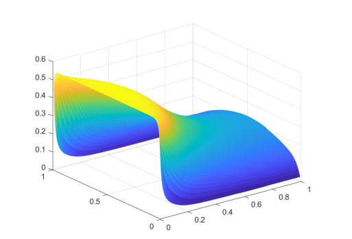
For the time-dependent case, we set \[\nu=0.0055,\qquad T=1,\qquad \hat{u}_0\equiv 0.55,\qquad \hat{P}_0=0.35,\qquad \hat{P}_1=0.125, \qquad \text{in }[0,1]\times[0,T].\] Moreover, we define \[m_{10}=300, \qquad \Delta t=d_2=\frac{T}{m_{10}},\] and \[t_k=k\Delta t=kd_2\in[0,T], \qquad \forall k=1,\ldots,m_{10}.\]
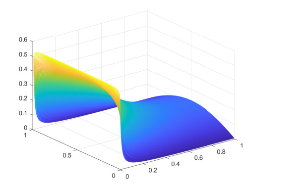
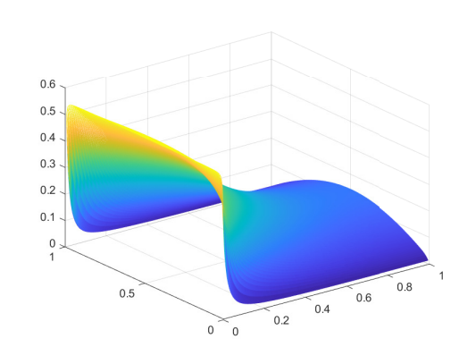
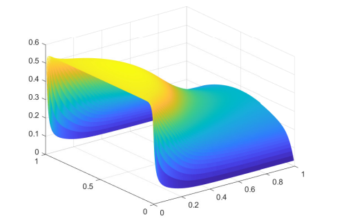
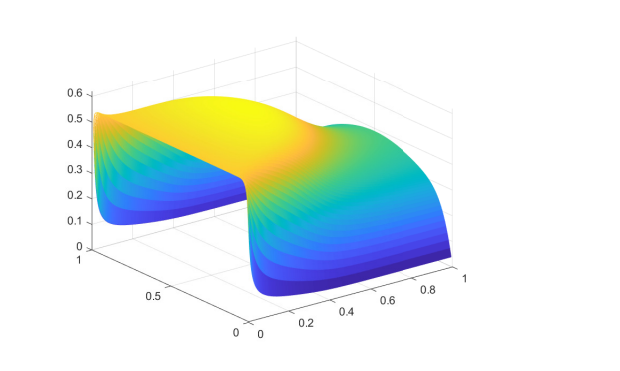
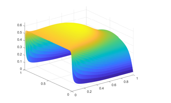
We also set an initial solution \((u_0^*,v_0^*)\) corresponding to a solution of the time-independent case with \(\nu=0.55\). For the graph of this initial solution \(u_0^*\), see Figure 7. For the solutions of the velocity field \(u=u(x,y,t)\) corresponding to the time levels \(u_{20}(x,y)\), \(u_{100}(x,y)\), \(u_{150}(x,y)\), \(u_{250}(x,y)\), and \(u_{299}(x,y)\), see Figures 8, 9, 10, 11, and 12, respectively.
We now present the MATLAB implementation through which these
numerical results were obtained. The main program for the
time-independent case, which is also used to obtain the initial solution
for the time-dependent case, is entitled
LinesNavierStokesJanuray2026B and is given below.
clear all

global u5 v5 P5

m8=800;
%m8=1200;
%m8=1600;

m9=120;

d=1/m8;

d1=1/m9;

%e1=0.03;

e1=0.55;

e2=1.0;

%K=50;

K=120;

Id=eye(m9-1);

m2=zeros(m9-1,m9-1);

for i=2:m9-2

m2(i,i)=-2.0;

m2(i,i+1)=1.0;

m2(i,i-1)=1.0;

end;

m2(1,1)=-2.0;

m2(1,2)=1;

m2(m9-1,m9-1)=-2.0;

m2(m9-1,m9-2)=1.0;

m22=zeros(m9-1,m9-1);

for i=2:m9-2

m22(i,i)=-2.0;

m22(i,i+1)=1.0;

m22(i,i-1)=1.0;

end;

m22(1,1)=-1.0;

m22(1,2)=1;

m22(m9-1,m9-1)=-1.0;

m22(m9-1,m9-2)=1.0;

m1=zeros(m9-1,m9-1);

for i=2:m9-2

m1(i,i)=-1;

m1(i,i+1)=1;

end;

m1(1,1)=-1;

m1(1,2)=1;

m1(m9-1,m9-1)=-1;

m1a=zeros(m9-1,m9-1);

for i=2:m9-1

m1a(i,i)=1;

m1a(i,i-1)=-1;

end;

m1a(1,1)=1;

m1=(m1+m1a)/2;

for i=1:m8

uo(:,i)=0.3*ones(m9-1,1);

vo(:,i)=0.1*ones(m9-1,1);

Po(:,i)=0.3*ones(m9-1,1);

u1(:,i)=0.3*ones(m9-1,1);

end;

uoo(:,1)=.55*ones(m9-1,1);

voo(:,1)=0.0*ones(m9-1,1);

Poo(:,1)=0.35*ones(m9-1,1);

for k3=1:1

%e1=e1*.92;

b21=1;

k1=1;

while (b21>10^(-4)) && (k1<12)

k1

k1=k1+1;

k=1;

b12=1;

while (b12>10^(-4)) && (k<535)

k

k=k+1;

i=1;

m12=2*Id-m2/d1^2*d^2+K*d^2*Id/e1;

m50(:,:,i)=inv(m12);

z1(:,i)=m50(:,:,i)*(K*uo(:,i)*d^2/e1 ...
-vo(:,i).*m1*(uo(:,i))/d1*d^2/e1 ...
+uoo(:,1)-(Po(:,i)-Poo(:,1))/d*d^2/e1 ...
-uo(:,i).*(uo(:,i)-uoo(:,i))/d*d^2/e1);

for i=2:m8-1

m12=2*Id-m2/d1^2*d^2-m50(:,:,i-1)+K*d^2/e1*Id;

m50(:,:,i)=inv(m12);

z1(:,i)=m50(:,:,i)*(K*uo(:,i)*d^2/e1 ...
-vo(:,i).*m1*(uo(:,i))/d1*d^2/e1 ...
-(Po(:,i)-Po(:,i-1))/d*d^2/e1 ...
-uo(:,i).*(uo(:,i)-uo(:,i-1))/d*d^2/e1 ...
+z1(:,i-1));

end;

u(:,m8,1)=inv(Id-m50(:,:,m8-1))*z1(:,m8-1);

for i=1:m8-1

u(:,m8-i,1)=m50(:,:,m8-i)*u(:,m8-i+1,1)+z1(:,m8-i);

end;

b12=max(max(abs(u-uo)));

uo=u;

uo(m9/2,m8/2)

end;

k=1;

b14=1;

while (b14>10^(-4)) && (k<535)

k

k=k+1;

i=1;

m12=2*Id-m2/d1^2*d^2+K*d^2/e1*Id;

m60(:,:,i)=inv(m12);

z2(:,i)=m60(:,:,i)*(K*vo(:,i)*d^2/e1 ...
-vo(:,i).*m1*(vo(:,i))/d1*d^2/e1 ...
-(uo(:,i)).*(vo(:,i)-voo(:,i))/d*d^2/e1 ...
+voo(:,1)-m1*(Po(:,i))/d1*d^2/e1);

for i=2:m8-1

m12=2*Id-m2/d1^2*d^2-m60(:,:,i-1)+K*d^2*Id/e1;

m60(:,:,i)=inv(m12);

z2(:,i)=m60(:,:,i)*(K*vo(:,i)*d^2/e1 ...
-vo(:,i).*m1*(vo(:,i))/d1*d^2/e1 ...
-m1*(Po(:,i))/d1*d^2/e1+z2(:,i-1) ...
-(uo(:,i)).*(vo(:,i)-vo(:,i-1))/d*d^2/e1);

end;

v(:,m8,1)=inv(Id-m60(:,:,m8-1))*z2(:,m8-1);

for i=1:m8-1

v(:,m8-i,1)=m60(:,:,m8-i)*v(:,m8-i+1)+z2(:,m8-i);

end;

b14=max(max(abs(v-vo)));

vo=v;

vo(m9/2,m8/2)

end;

b18=1;

k=1;

while (b18>10^(-4)) && (k<535)

k

k=k+1;

i=1;

m12=2*Id-m22/d1^2*d^2+K*Id*d^2;

d1uo(:,1)=(uo(:,i)-uoo(:,1))/d;

d2uo(:,1)=m1*uo(:,i)/d1;

d1vo(:,1)=(vo(:,i)-voo(:,1))/d;

d2vo(:,1)=m1*vo(:,i)/d1;

m80(:,:,i)=inv(m12);

z3(:,i)=m80(:,:,i)*(K*Po(:,i)*d^2+Poo(:,1) ...
+d1uo(:,1).*d1uo(:,1)*d^2 ...
+d2vo(:,1).*d2vo(:,1)*d^2 ...
+2*d2uo(:,1).*d1vo(:,1)*d^2);

for i=2:m8-1

m12=2*Id-m22/d1^2*d^2+K*Id*d^2-m80(:,:,i-1);

d1uo(:,1)=(uo(:,i)-uo(:,i-1))/d;

d2uo(:,1)=m1*uo(:,i)/d1;

d1vo(:,1)=(vo(:,i)-vo(:,i-1))/d;

d2vo(:,1)=m1*vo(:,i)/d1;

m80(:,:,i)=inv(m12);

z3(:,i)=m80(:,:,i)*(K*Po(:,i)*d^2 ...
+d1uo(:,1).*d1uo(:,1)*d^2 ...
+d2vo(:,1).*d2vo(:,1)*d^2 ...
+2*d2uo(:,1).*d1vo(:,1)*d^2+z3(:,i-1));

end;
%P(:,m8)=inv(Id-m80(:,:,m8-1))*z3(:,m8-1);

P(:,m8,1)=0.125*ones(m9-1,1);
%P(:,m8)=0.08*ones(m9-1,1);

for i=1:m8-1

P(:,m8-i,1)=m80(:,:,m8-i)*P(:,m8-i+1,1)+z3(:,m8-i);

end;

b18=max(max(abs(P(:,:,1)-Po)));

Po=P(:,:,1);

Po(m9/2,m8/2)

end;

b21=max(max(abs(uo-u1)));

u1=uo;

end;

% C1(1,1)=b12;C1(2,1)=b14;C1(3,1)=b18;

end;

u5=uo;

v5=vo;

P5=Po;

for i=1:m8

x1(i,1)=i*d;

end;

for i=1:m9-1

x2(i,1)=i*d1;

end;

mesh(x1,x2,u(:,:,1))
The main program for the time-dependent case is entitled
LinesNavierStokesJanuary2026TD1 and is given below.
global u5 v5 P5

m8=800;
%m8=1200;
%m8=1600;

m9=120;
%m10=200;

m10=300;
%d2=0.5/m10;

d2=1/m10;

d=1/m8;

d1=1/m9;
%e1=0.0005;
%e1=0.00020;

e1=0.0055;

e2=1.0;

e3=0.03;
%K=0;

K=180;

Id=eye(m9-1);

m2=zeros(m9-1,m9-1);

for i=2:m9-2

m2(i,i)=-2.0;

m2(i,i+1)=1.0;

m2(i,i-1)=1.0;

end;

m2(1,1)=-2.0;

m2(1,2)=1;

m2(m9-1,m9-1)=-2.0;

m2(m9-1,m9-2)=1.0;

m22=zeros(m9-1,m9-1);

for i=2:m9-2

m22(i,i)=-2.0;

m22(i,i+1)=1.0;

m22(i,i-1)=1.0;

end;

m22(1,1)=-1.0;

m22(1,2)=1;

m22(m9-1,m9-1)=-1.0;

m22(m9-1,m9-2)=1.0;

m1=zeros(m9-1,m9-1);

for i=2:m9-2

m1(i,i)=-1;

m1(i,i+1)=1;

end;

m1(1,1)=-1;

m1(1,2)=1;

m1(m9-1,m9-1)=-1;

m1a=zeros(m9-1,m9-1);

for i=2:m9-1

m1a(i,i)=1;

m1a(i,i-1)=-1;

end;

m1a(1,1)=1;

m1=(m1+m1a)/2;

for i=1:m8

uo(:,i)=u5(:,i);

vo(:,i)=v5(:,i);

Po(:,i)=P5(:,i);

u1(:,i)=0.3*ones(m9-1,1);

end;

for i=1:m8

u(:,i,1)=u5(:,i);

v(:,i,1)=v5(:,i);

P(:,i,1)=P5(:,i);

u1(:,i)=0.3*ones(m9-1,1);

end;

uoo(:,1)=.55*ones(m9-1,1);

voo(:,1)=0.0*ones(m9-1,1);

Poo(:,1)=0.35*ones(m9-1,1);

%b12=1;

%b14=1;
%b18=1;
%k=1;
%C1(1,1)=b12;C1(2,1)=b14;C1(3,1)=b18;

for k3=1:1
%e1=e1*.92;

for j=2:m10-1

b21=1;

k1=1;

%while (b21>10^(-4)) & (k1<8)

while (b21>10^(-4)) && (k1<32)

k1

k1=k1+1;

k=1;

b12=1;

while (b12>10^(-4)) && (k<535)

k

k=k+1;

i=1;

%v1(:,i)=-(1-e3)*(uo(:,i+1)-2*uo(:,i)+uoo(:,1)+m2*uo(:,i)/d1^2*d^2);

m12=2*Id-m2/d1^2*d^2+Id/d2/e1*d^2;

m50(:,:,i)=inv(m12);

z1(:,i)=m50(:,:,i)*(uoo(:,1)+u(:,i,j-1)/d2*d^2/e1 ...
-(vo(:,i)).*m1*uo(:,i)/d1*d^2/e1 ...
-((uo(:,i)-uoo(:,i))).*uo(:,i)/d*d^2/e1 ...
-(Po(:,i)-Poo(:,1))/d*d^2/e1);

for i=2:m8-1
% v1(:,i)=-(1-e3)*(uo(:,i+1)-2*uo(:,i)+uo(:,i-1)+m2*uo(:,i)/d1^2*d^2);

m12=2*Id-m2/d1^2*d^2-m50(:,:,i-1)+Id/d2*d^2/e1;

m50(:,:,i)=inv(m12);

z1(:,i)=m50(:,:,i)*(u(:,i,j-1)/d2*d^2/e1 ...
-(vo(:,i)).*(m1*uo(:,i))/d1*d^2/e1 ...
-((uo(:,i)-uo(:,i-1))).*uo(:,i)/d*d^2/e1 ...
-(Po(:,i)-Po(:,i-1))/d*d^2/e1+z1(:,i-1));

end;

u(:,m8,j)=inv(Id-m50(:,:,m8-1))*z1(:,m8-1);

for i=1:m8-1

u(:,m8-i,j)=m50(:,:,m8-i)*u(:,m8-i+1,j)+z1(:,m8-i);

end;

b12=max(max(abs(u(:,:,j)-uo)));

uo=u(:,:,j);

uo(m9/2,m8/2)

end;

k=1;

b14=1;

while (b14>10^(-4)) && (k<535)

k

k=k+1;

i=1;

%v2(:,i)=-(1-e3)*(vo(:,i+1)-2*vo(:,i)+voo(:,1)+m2*vo(:,i)/d1^2*d^2);

m12=2*Id-m2/d1^2*d^2+Id/d2*d^2/e1;

m60(:,:,i)=inv(m12);

z2(:,i)=m60(:,:,i)*(voo(:,1) ...
-(vo(:,i)).*m1*vo(:,i)/d1*d^2/e1 ...
-(uo(:,i)).*(vo(:,i)-voo(:,i))/d*d^2/e1 ...
+v(:,i,j-1)/d2/e1*d^2-m1*(Po(:,i))/d1*d^2/e1);

for i=2:m8-1

% v2(:,i)=-(1-e3)*(vo(:,i+1)-2*vo(:,i)+vo(:,i-1)+m2*vo(:,i)/d1^2*d^2);

m12=2*Id-m2/d1^2*d^2-m60(:,:,i-1)+Id/d2*d^2/e1;

m60(:,:,i)=inv(m12);

z2(:,i)=m60(:,:,i)*(+v(:,i,j-1)/d2/e1*d^2 ...
-(vo(:,i)).*m1*vo(:,i)/d1*d^2/e1 ...
-(uo(:,i)).*(vo(:,i)-vo(:,i-1))/d*d^2/e1 ...
-m1*(Po(:,i))/d1*d^2/e1);

end;

v(:,m8,j)=inv(Id-m60(:,:,m8-1))*z2(:,m8-1);

for i=1:m8-1

v(:,m8-i,j)=m60(:,:,m8-i)*v(:,m8-i+1,j)+z2(:,m8-i);

end;

b14=max(max(abs(v(:,:,j)-vo)));

vo=v(:,:,j);

vo(m9/2,m8/2)

end;

b18=1;

k=1;

while (b18>10^(-4)) && (k<535)

k

k=k+1;

i=1;

m12=2*Id-m22/d1^2*d^2+K*Id*d^2;

d1uo(:,1)=(uo(:,i)-uoo(:,1))/d;

d2uo(:,1)=m1*uo(:,i)/d1;

d1vo(:,1)=(vo(:,i)-voo(:,1))/d;

d2vo(:,1)=m1*vo(:,i)/d1;

m80(:,:,i)=inv(m12);

z3(:,i)=m80(:,:,i)*(K*Po(:,i)*d^2+Poo(:,1) ...
+d1uo(:,1).*d1uo(:,1)*d^2 ...
+d2vo(:,1).*d2vo(:,1)*d^2 ...
+2*d2uo(:,1).*d1vo(:,1)*d^2);

for i=2:m8-1

m12=2*Id-m22/d1^2*d^2+K*Id*d^2-m80(:,:,i-1);

d1uo(:,1)=(uo(:,i)-uo(:,i-1))/d;

d2uo(:,1)=m1*uo(:,i)/d1;

d1vo(:,1)=(vo(:,i)-vo(:,i-1))/d;

d2vo(:,1)=m1*vo(:,i)/d1;

m80(:,:,i)=inv(m12);

z3(:,i)=m80(:,:,i)*(K*Po(:,i)*d^2 ...
+d1uo(:,1).*d1uo(:,1)*d^2 ...
+d2vo(:,1).*d2vo(:,1)*d^2 ...
+2*d2uo(:,1).*d1vo(:,1)*d^2+z3(:,i-1));

end;
%P(:,m8,j)=inv(Id-m80(:,:,m8-1))*z3(:,m8-1);

P(:,m8,j)=0.125*ones(m9-1,1);
%P(:,m8)=0.08*ones(m9-1,1);

for i=1:m8-1

P(:,m8-i,j)=m80(:,:,m8-i)*P(:,m8-i+1,j)+z3(:,m8-i);

end;

b18=max(max(abs(P(:,:,j)-Po)));

Po=P(:,:,j);

Po(m9/2,m8/2)
end;

b21=max(max(abs(uo-u1)));

u1=uo;

end;

%C1(1,1)=b12;C1(2,1)=b14;C1(3,1)=b18;

end;

end;

for i=1:m8

x1(i,1)=i*d;

end;

for i=1:m9-1

x2(i,1)=i*d1;

end;

mesh(x1,x2,u(:,:,20))
The objective of this section is complete.
In this article, we have presented a numerical procedure for solving a large class of partial differential equations, specifically for a non-circular simply connected domain in a Cartesian-coordinate context. Although we have applied the method to a Navier–Stokes type equation, we emphasize that this method may be extended to a large class of other linear and nonlinear partial differential equations. In future research, we intend to address several other linear and nonlinear cases.