
The Laplace transform has emerged as a central tool in the study of stochastic processes, with particular importance in the analysis of renewal processes. By transforming differential equations into the “s” domain, it simplifies complex calculations and facilitates the computation of transfer functions and system characteristics. This transformation allows researchers to move from the time domain to the Laplace domain, perform structured analyses, and subsequently return to the time domain to obtain concrete and applicable solutions.
In the context of stochastic processes, the Laplace transform enables deeper insights and provides solutions to equations describing the evolution of complex random systems. As demonstrated by Ahmed [1], this approach often offers alternative, and sometimes simplified, perspectives on process behavior. Specifically, in renewal processes, it proves effective for analyzing the intervals between events, offering a robust framework for systems where event occurrences are irregular.
Sub-Gaussian random variables, widely applied across diverse fields, are closely related to Laplace transforms. Introduced by Kahane [2] in the study of Fourier random series convergence (see also Buldygin et al. [3]), a variable is considered sub-Gaussian if its Laplace transform is dominated by that of a centered Gaussian variable. Consequently, every sub-Gaussian variable is centered, and its variance is bounded by the standard deviation of the corresponding Gaussian variable.
Reliability assessment has become an essential aspect of quality management in industrial production. Evaluating the reliability of complex systems requires accurate estimation of component operating times and a detailed analysis of system failure sequences. Such analyses enable the development of models for quantitative reliability evaluation [4]. Among mathematical tools used in this field, the Laplace transform is particularly significant for system reliability and availability analysis [5]. This article aims to present a concrete application of the Laplace transform in reliability assessment.
Nevertheless, determining the Laplace transform for certain probability distributions can be challenging or, in some cases, impossible. This article explores the main properties of the Laplace transform while providing numerous examples illustrating its application to simple and complex distributions. The structure of the space of Laplace transforms is also examined due to its relevance in reliability studies. Results are expressed in explicit formulas or using well-established special functions. Finally, an application to a renewal process is presented, demonstrating the crucial role of the Laplace transform in simplifying complex calculations.
Definition 1. The Laplace transform of a function \(f(x)\) (possibly generalized, such as the “Dirac function”) of a real variable \(t\), with positive support, is the function \(L_f\) of the strictly positive real variable \(s\), defined by (see Rainville [6] or Widder [7]): \[\label{laplace} L_f(s)=\displaystyle\int_0^{+\infty}f(x)e^{-sx}dx. \tag{1}\]
We could also be interested in the Laplace-Stieltjes transform.
Definition 2. The Laplace-Stieltjes transform of a funcfion \(f(x)\), denoted \(L_f^\star\), is defined by (see Apostol [8] or Ross [9]) \[L_f^\star(s)=\displaystyle\int_0^{+\infty}e^{-sx}dF(x), \tag{2}\] where \(F'(x)=f(x)\).
The Laplace-Stieltjes transform is used to transform functions which possess both discrete and continuous parts and is reduced to the standard Laplace transform (1) in the fully continuous case.
We will investigate the Laplace transform on probability density distributions with positive support and also study its convergence.
Proposition 1. If \(f(x)\) is probability density distribution with positive support, then the improper integral of \(f(x)\) given by (see Widder [7]) \[\displaystyle\int_0^{+\infty}f(x)e^{-sx}dx, \tag{3}\] converges uniformly for all positive \(s\).
This result shows that the Laplace transform of probability density distribution function with positive support, exists for al1 positive \(s\). Further, it is the case that, \(0\leqslant L_f(s) \leqslant 1,\quad\forall s\geqslant 0\).
Let \(X\) and \(Y\) be two independent absolutely continuous random variables, with positive support, with joint distribution \(h(x,y)\) and respective probability density functions \(f(x)\) and \(g(y)\). Then we have: \[\mathbb{P}(Y>X)=\displaystyle\int_0^{+\infty}\int_x^{+\infty}h(x,y) dy dx =\displaystyle\int_0^{+\infty}\mathbb{P}(Y>x)f(x) dy dx.\]
The Laplace transform of a probability density can be interpreted as the probability that a random variable \(Y\), following an exponential distribution, “dominates” another random variable \(X\) whose density is given by \(f(x)\). For example, in statistics, if we consider that \(Y\) represents the lifetime of a device while \(X\) corresponds to its first failure, the Laplace transform of \(f(x)\), in this context, represents the probability that the device continues to work after this first failure. On this basis, we propose analogous interpretations of certain properties of the Laplace transform, which will prove to be very useful for the further development of our study.
Proposition 2. Let \(X\) and \(Y\) be two independent continuous random variables such that \(Y\rightsquigarrow \mathcal{E}(s)\), exponential distribution and \(X\) has probability density function \(f(x)\). Then, we have (see Foran [10]) \[\label{Lproba} L_f(s)=\mathbb{P}(Y>X). \tag{4}\]
As a consequence of the proposition stated previously, we present the relation which establishes a link between the Laplace transform of a probability function \(f(x)\) and that of its distribution function \(F(x)\).
Corollary 1. Under the same assumptions as Proposition 2, if \(F(x)\) is the cumulative distribution function of X and \(f(x)\) its probability density, then we get: \[\label{LF_Lf} L_f(s)=sL_F(s), \tag{5}\] where \(L_F\) is the Laplace transform of \(F(x)\).
Defintion 3. Consider a random variable \(X\). The distribution of \(X\) is said to be memoryless if for all \(n, m >0\), we have \[\mathbb{P}(X \geqslant s + t | X \geqslant s) = \mathbb{P}(X \geqslant t).\]
The memory loss property is characteristic of certain probability distributions, such as the exponential distribution and the geometric distribution. These are referred to as memoryless distributions.
Proposition 3. Let \(X,Y\) and \(Z\) be three independent continuous random variables such that \(Y\rightsquigarrow \mathcal{E}(\lambda)\), \(X\) and \(Z\) have respectively probability density functions \(f(x)\) and \(g(z)\). Then, we get: \[\mathbb{P}(Y>X+Z | Y>X)=\mathbb{P}(Y>Z). \tag{6}\]
Another way to interpret the memory loss property is to state that the distribution of survival time until the next occurrence of an event in a memoryless process remains the same, regardless of how long one has already waited before that event. In other words, the probability of the event occurring in a given time interval does not vary depending on how long one has already waited, which underlines the independence of future events from the history of past events.
Corollary 2. Let \(X_1 \cdots X_n\) be a sequence of random variables independent of respective probability density functions \((f_i(x_i))_{i=1}^n\), and let \(Y\) be a random variable with exponential distribution, independent of \((X_i)_{i=1}^n\). We set \(\Sigma_n=X_1+ \cdots +X_n=\displaystyle\sum_{i=1}^n X_i\) and we denote by \(f_{\Sigma_n}(x)\) its probability density function. Then we have (Hogg and Craig [11]): \[f_{\Sigma_n}(s)=\displaystyle\prod_{i=1}^n f_i(s). \tag{7}\]
Proposition 4. The following integral representations of gamma functions (or Euler’s integral) are equivalent for \(s>0\):
\(\circ\) \(\Gamma(s)=\displaystyle\int_0^{+\infty}t^{s-1}e^{-t}dt\),
\(\circ\) \(\Gamma(s)=x^s\displaystyle\int_0^{+\infty}t^{s-1}e^{-xt}dt\quad\forall x > 0\),
\(\circ\) \(\Gamma(s)=\displaystyle\int_{-\infty}^{+\infty}\exp(st – e^{-t})dt\).
Proof. The proof of this proposition can be found in Gradshteyn and Ryzhik [12]. ◻
Notation 1. The upper incomplete gamma function is defined as: \(\gamma(a,x)=\displaystyle\int_{0}^x t^{a-1}e^{-t}dt\), whereas the lower incomplete gamma function is defined as: \(\Gamma(a,x)=\displaystyle\int_x^{+\infty} t^{a-1}e^{-t}dt\).
Based on all the concepts previously presented, we will calculate the Laplace transforms of the most significant probability density functions as well as the most commonly encountered distributions. In the following development, we assume that the random variable \(Y\), which follows an exponential distribution denoted by \(\mathcal{E}(s)\), is independent of the random variable \(X\) whose density is designated by \(f(x)\). The calculations of the Laplace transforms will be carried out either directly using the formula (1), or by resorting to the formula (4), or by means of the formula for moment generating functions, the definition of which we will provide in a later section of this document.
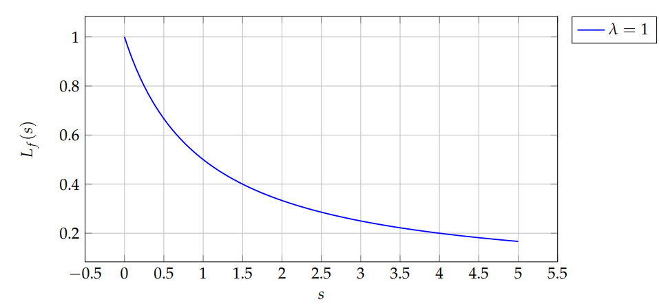
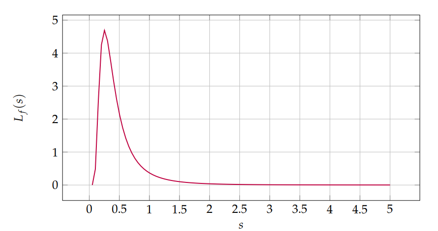
Theorem 1. If X is an exponential distribution i.e. \(X\rightsquigarrow\mathcal{E}(\lambda)\) with density \(f(x)=\lambda e^{-\lambda x}\mathbf{l}_{\{x \geqslant 0\}}\), then we have: \[L_f(s)=\displaystyle\frac{\lambda}{\lambda + s}. \tag{8}\]
Proof. \(L_f(s)=\displaystyle\int_0^{+\infty}\lambda e^{-\lambda x} e^{-s x}dx=\displaystyle\int_0^{+\infty}\lambda e^{-(\lambda +s)x}dx=\displaystyle\frac{\lambda}{\lambda + s}\). ◻
For \(\lambda=1\), \(L_f(s)=1/(1+s)\). Figure 1 shows \(L_f(s)\).
Corollary 3. If \(X\) is a hyperexponential distribution, i.e. \(X\rightsquigarrow\mathcal{H}_n(p_i;\lambda_i)\), with density \[f(x)=\displaystyle\sum_{i=1}^n p_i\lambda_i e^{-\lambda_i x}\mathbf{l}_{\{x \geqslant 0\}},\] where \(\displaystyle\sum_{i=1}^n p_i=1\) and \(\lambda_i,p_i>0\), then we have: \[L_f(s)=\displaystyle\sum_{i=1}^np_i\frac{\lambda_i}{\lambda_i + s}. \tag{9}\]
Proof. It suffices to notice that \(f(x)=\displaystyle\sum_{i=1}^np_i f_i(x)\) where \(f_i(x)\) is the density of the exponential distribution with parameter \(\lambda_i\). Using the linearity of the Laplace transform and Theorem 1, we obtain \[L_f(s)=\displaystyle\sum_{i=1}^np_i L_{f_i}(s)=\displaystyle\sum_{i=1}^np_i\frac{\lambda_i}{\lambda_i + s}.\] ◻
Corollary 4. If \(X\) is a hypoexponential distribution, i.e. \(X\rightsquigarrow\mathcal{H}_n(\lambda_i)\), with density \[f(x)=\displaystyle\sum_{i=1}^n \prod_{i\neq j}\frac{\lambda_j}{\lambda_j – \lambda_i}\lambda_i e^{-\lambda_i x}\mathbf{l}_{\{x \geqslant 0\}},\] where \(\lambda_i>0\), then we have: \[L_f(s)=\displaystyle\sum_{i=1}^n \prod_{i\neq j}\frac{\lambda_i\lambda_j}{(\lambda_j – \lambda_i)(\lambda_i + s)}. \tag{10}\]
Proof. The proof of this corollary is similar to that of Corollary 3 by replacing \(p_i\) by the constant \[p_{ij}=\displaystyle\prod_{i\neq j}\frac{\lambda_j}{\lambda_j – \lambda_i}.\] ◻
Theorem 2. If \(X\) is a generalized Erlang distribution denoted by \(\Gamma(n,\lambda_i),\, 1\leqslant i \leqslant n\), i.e. \(X=\displaystyle\sum_{i=1}^n X_i\) and \((X_i)_{i=1}^n\) is a sequence of independent random variables with exponential distributions such that \(X_i\rightsquigarrow \mathcal{E}(\lambda_i)\)with respective densities \(f_i\), then we have: \[L_f(s)=\displaystyle\prod_{i=1}\frac{\lambda_i}{\lambda_i + s}. \tag{11}\]
Proof. The proof of this theorem is based on the combination of Corollary 2 and Theorem 1. Indeed, we have: \[L_f(s)=\mathbb{P}(Y>X)=\mathbb{P}\left(Y>\displaystyle\sum_{i=1}^n X_i\right)=\displaystyle\prod_{i=1}^n L_{f_i}(s)=\displaystyle\prod_{i=1}^n\frac{\lambda_i}{\lambda_i + s}.\] ◻
Corollary 5. If \(X\) is a Erlang distribution, i.e. \(X\rightsquigarrow\Gamma(n,\lambda)\), with density \[f(x)=\displaystyle\frac{\lambda^n}{\Gamma(n)}x^{n-1}e^{-\lambda x}\mathbf{l}_{\{x \geqslant 0\}},\] then we obtain \[L_f(s)=\displaystyle\left(\frac{\lambda}{\lambda + s}\right)^n. \tag{12}\]
Proof. The proof of this corollary is deduced from Theorem 2 by noticing that the Erlang distribution is a particular case of the generalized Erlang distribution with the constants \(\lambda_i,\;1\leqslant i \leqslant n\), identical and all equal to \(\lambda\) i.e., we get \(L_f(s)=\displaystyle\prod_{i=1}\frac{\lambda}{\lambda + s}\). ◻
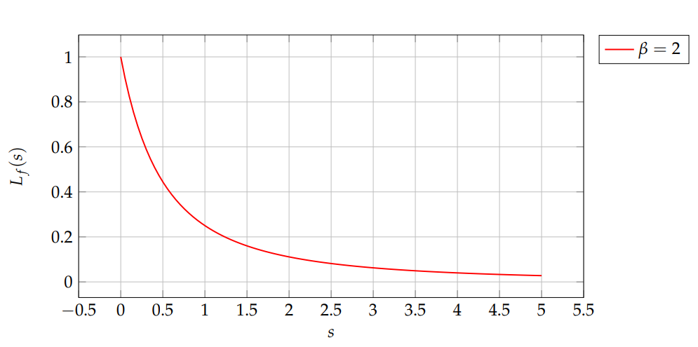
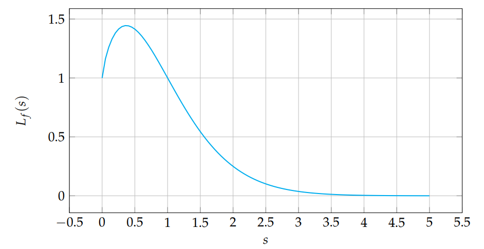
Corollary 6. If \(X\) is a Gamma distribution, i.e. \(X\rightsquigarrow\mathcal{G}(\beta,\lambda)\), with density \[f(x)=\displaystyle\frac{\lambda^\beta}{\Gamma(\beta)}x^{\beta-1}e^{-\lambda x}\mathbf{l}_{\{x \geqslant 0\}},\] then \[L_f(s)=\displaystyle\left(\frac{\lambda}{\lambda + s}\right)^\beta. \tag{13}\]
Proof. The proof of this corollary follows from Corollary 5 by noticing that the Gamma distribution is a generalized case of the Erlang distribution with \(n=\beta>0\). ◻
Let \(\beta=2\), \(\lambda=1\), then \(L_f(s)=(1/(1+s))^2\). Figure 2 shows the transform.
Corollary 7. If \(X\) is a chi-squared distribution, i.e. \(X\rightsquigarrow\chi^2(n)\), with density \[f(x)=\displaystyle\frac{\lambda^{\frac{n}{2}}}{\Gamma\left(\displaystyle\frac{n}{2}\right)}x^{\frac{n}{2}-1}e^{-\lambda x}\mathbf{l}_{\{x \geqslant 0\}},\] then \[L_f(s)=\displaystyle\frac{1}{(1 + 2s)^{\frac{n}{2}}}. \tag{14}\]
Proof. It is sufficient to notice that the chi-squared distribution is special case of the gamma distribution with \(\lambda=\displaystyle\frac{1}{2}\) and \(\beta=\displaystyle\frac{n}{2}\). The conclusion follows from Corollary 6. ◻
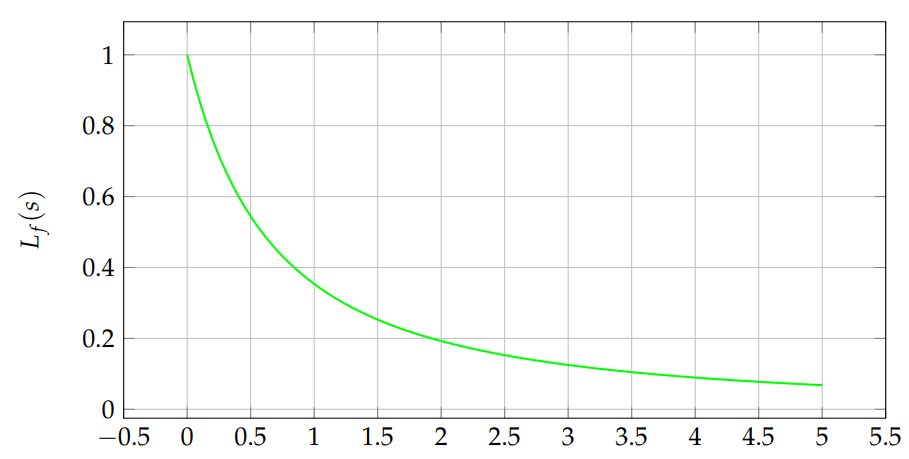
Theorem 3. If \(X\) is a Weibull distribution, i.e. \(X\rightsquigarrow\mathcal{W}(\alpha,\beta)\), with density \[f(x)=\alpha\beta x^{\alpha – 1}\exp\left(-\beta x^\alpha\right)\mathbf{l}_{\{x \geqslant 0\}},\\ \forall \alpha,\beta > 0,\] then we have \[L_f(s)=\displaystyle\sum_{n\geqslant 0}(-1)^n\frac{\Gamma\left(1+\frac{n}{\alpha}\right)}{\beta^{\frac{n}{\alpha}}}. \tag{15}\]
Proof. Note that the moment-generating function \(M_X\) for a positive random variable \(X\) is defined by the relation \[M_X(s)=\mathbb{E}\left[e^{sX}\right]=\displaystyle\int_0^{+\infty}f(x)e^{sx}dx.\]
Moreover we have \(\mathbb{E}(X^n)=M_X^{(n)}(0)\) where \(M_X^{(n)}(t)=\displaystyle\frac{d^n}{dt^n}M_X(t)\). So, we can write \[\begin{aligned} M_X(s)=&\displaystyle\int_0^{+\infty}e^{sx}\alpha\beta x^{\alpha – 1}\exp\left(\beta x^\alpha\right) dx\\ =&\displaystyle\int_0^{+\infty}\alpha\beta x^{\alpha – 1}\exp\left(-\beta x^\alpha + sx\right) dx.\\ \end{aligned}\]
By the Leibniz integral rule, we get \[M_X^{(n)}(s)=\alpha\beta\displaystyle\int_0^{+\infty}\frac{\partial^n}{\partial s^n}\left( x^{\alpha – 1}\exp\left(-\beta x^\alpha + sx\right) \right)dx=\alpha\beta\displaystyle\int_0^{+\infty}x^{\alpha + n – 1}\exp\left(-\beta x^\alpha + sx\right),\] so \[M_X^{(n)}(0)=\alpha\beta\displaystyle\int_0^{+\infty}x^{\alpha + n – 1}\exp\left(-\beta x^\alpha\right).\]
Using the change of variable \(u=\beta x^\alpha\), we have \[M_X^{(n)}(0)=\displaystyle\frac{1}{\beta^{\frac{n}{\alpha}}}\int_0^{+\infty}u^{\frac{n}{\alpha}}e^{-u}du=\displaystyle\frac{\Gamma\left(1+\frac{n}{\alpha}\right)}{\beta^{\frac{n}{\alpha}}}.\]
Moreover, with the Taylor series of the exponential map, we have \[\label{Mx} M_X(s)=\mathbb{E}\left[e^{sX}\right]=\mathbb{E}\left[\displaystyle\sum_{n\geqslant 0}X^n \frac{s^n}{n!}\right]=\displaystyle\sum_{n\geqslant 0}\mathbb{E}\left[X^n\right]\frac{s^n}{n!}=\displaystyle\sum_{n\geqslant 0}M_X^{(n)}(0)\frac{s^n}{n!}=\displaystyle\sum_{n\geqslant 0}\displaystyle\frac{\Gamma\left(1+\frac{n}{\alpha}\right)}{\beta^{\frac{n}{\alpha}}}\frac{s^n}{n!}. \tag{16}\]
Formula (16) completes this proof just by noticing that \(L_f(s)=M_X(-s)\). ◻
For \(\alpha=2\), \(\beta=1\) (Rayleigh), numerical integration can be used. Figure 3 shows the shape.
Theorem 4. If \(X\) is a Pareto distribution, i.e. \(X\rightsquigarrow\mathcal{P}(\alpha,\beta)\), with density \(f(x)=\displaystyle\frac{\alpha\beta^\alpha}{x^{\alpha + 1}}\mathbf{l}_{\{x \geqslant \beta\}},\, \forall \alpha,\beta > 0\), then we have \[L_f(s)=\alpha(\alpha\beta)^\alpha\gamma(-\alpha,\beta s),\quad\text{where}\quad\gamma(a,b)=\displaystyle\int_b^{+\infty}u^{a-1}e^{-u}du. \tag{17}\]
Proof. \[\begin{aligned} L_f(s)=&\displaystyle\int_\beta^{+\infty}\frac{\alpha\beta^\alpha}{x^{\alpha + 1}}e^{-sx}dx,\\ =&\alpha(\alpha\beta)^\alpha\displaystyle\int_{\beta s}^{+\infty}u^{-\alpha – 1}e^{-u}du,\;\text{after using the change of variable}\; u=sx. \end{aligned}\] ◻
Theorem 5. If \(X\) is a Logistic distribution, i.e. \(X\rightsquigarrow\mathcal{L}(m,\sigma)\), with density \(f(x)=\displaystyle\frac{1}{\sigma}\frac{\exp\left(-\frac{x – m}{\sigma}\right)}{\left[1 + \exp\left(-\frac{x – m}{\sigma}\right)\right]^2},\;\) where \(m\in\mathbb{R},\sigma > 0\), then we have \[L_f(s)=\displaystyle\frac{1}{e^{ms}}\sum_{n\geqslant 0}\frac{(-1)^nE_n(0)\Gamma(n+1,-sm)}{n!(s\sigma)^n}, \tag{18}\] where \(E_n(x)=\displaystyle\sum_{k=0}^n C_n^k\frac{E_k}{2^k}\left(x – \frac{1}{2}\right)^{n-k}\) and \((E_k)_{k=0}^n\) are the Euler numbers such that \(\displaystyle\frac{1}{\cosh t}=\displaystyle\frac{2}{e^t + e^{-t}}=\sum_{k=0}^\infty \displaystyle\frac{E_k}{k!}t^k\).
Proof. Note that the cumulative distribution function is \(F(x)=\displaystyle\frac{1}{1 + \exp\left(-\frac{x – m}{\sigma}\right)}\), and the generating function for the Euler polynomials is (see Tsuneo and al. [13]): \[\begin{aligned} \label{Euler} \displaystyle\frac{2e^{xt}}{e^t + 1}=\displaystyle\sum_{n\geqslant 0}E_n(x)\frac{t^n}{n!}. \end{aligned} \tag{19}\]
From Formula (19), we deduce that \(F(x)=\displaystyle\sum_{n\geqslant 0}\frac{(-1)^nE_n(0)}{n!2\sigma^n}(x-m)^n,\) and we can write \[\begin{aligned} L_F(s)=&\displaystyle\sum_{n\geqslant 0}\frac{(-1)^nE_n(0)}{n!2\sigma^n}\int_0^{+\infty}(x-m)^ne^{-sx}dx\\ =&\displaystyle\sum_{n\geqslant 0}\frac{(-1)^nE_n(0)\Gamma(n+1,-sm)}{n!2\sigma^ns^{n+1}e^{sm}},\;\text{after making the change of variable}\: v=s(x-m), \end{aligned}\] and (5) completes the proof. ◻
Theorem 6. If \(X\) is a Beta distribution, i.e. \(X\rightsquigarrow\mathcal{B}(\alpha,\beta)\), with density \(f(x)=\displaystyle\frac{1}{B(\alpha,\beta)}x^{\alpha – 1}(1 – x)^{\beta – 1}\mathbf{l}_{\{0\leqslant x\leqslant 1\}},\) where \(\alpha,\beta > 0\) and \(B\) is the Beta function, defined by \(B(p,q)=\displaystyle\int_0^1 t^{p-1}(1 – t)^{q – 1}dt\;p,q>0\), then we obtain \[L_f(s)=1+\displaystyle\sum_{n\geqslant 1}(-1)^n\frac{s^n}{n!}\prod_{k=0}^{n-1}\frac{\alpha + k}{\alpha + \beta +k}. \tag{20}\]
Proof. By using the Maclaurin series of the exponential function \(e^{-sx}\), we can write, \[\begin{aligned} L_f(s)=&\displaystyle\int_0^1 \displaystyle\frac{1}{B(\alpha,\beta)}x^{\alpha – 1}(1 – x)^{\beta – 1}e^{-sx}dx\\ =&\displaystyle\frac{1}{B(\alpha,\beta)}\sum_{n\geqslant 0}(-1)^n\frac{s^n}{n!}\int_0^1 x^{\alpha + n – 1}(1 – x)^{\beta – 1}dx\\ =& 1 + \displaystyle\sum_{n\geqslant 1}(-1)^n\frac{s^n}{n!}\frac{B(\alpha + n, \beta)}{B(\alpha,\beta)}, \end{aligned}\] and it must also be noted that \[\begin{aligned} \label{beta} \displaystyle\frac{B(\alpha + n, \beta)}{B(\alpha,\beta)}=&\displaystyle\frac{\Gamma(\alpha + n)\Gamma(\beta)\Gamma(\alpha + \beta)}{\Gamma(\alpha + \beta)\Gamma(\alpha)\Gamma(\beta)}\notag\\ =&\displaystyle\frac{\Gamma(\alpha)\displaystyle\prod_{k=0}^{n-1}(\alpha + k)\Gamma(\alpha + \beta)}{\Gamma(\alpha)\Gamma(\alpha + \beta)\displaystyle\prod_{k=0}^{n-1}(\alpha + \beta + k)}\notag\\ =&\displaystyle\prod_{k=0}^{n-1}\frac{\alpha + k}{\alpha + \beta + k}. \end{aligned} \tag{21}\]
Therefore, Formula (21) completes the proof. ◻
Theorem 7. If \(X\) is a Burr distribution, i.e. \(X\rightsquigarrow\mathcal{B}_r(c,\kappa)\), with density \(f(x)=c\kappa\displaystyle\frac{x^{c – 1}}{(1 + x^c)^{\kappa + 1}}\mathbf{l}_{\{x>0\}},\;\forall c,\kappa > 0,\) then we have \[L_f(s)=\kappa\displaystyle\sum_{n\geqslant 0}(-1)^n\frac{s^n}{n!}B\left(1 +\frac{n}{c}, \kappa – \frac{n}{c}\right), \tag{22}\] where \(B\) is the Beta function.
Proof. Using the Taylor series representation of the exponential function \(e^{-sx}\), we have \[\begin{aligned} L_f(s)=&c\kappa\displaystyle\int_0^{+\infty}\frac{x^{c – 1}}{(1 + x^c)^{\kappa + 1}}e^{-sx}dx\\ =&c\kappa\displaystyle\sum_{n\geqslant 0}(-1)^n\frac{s^n}{n!}\int_0^{+\infty}\frac{x^{n + c – 1}}{(1 + x^c)^{\kappa + 1}}dx \\ =& \kappa\displaystyle\sum_{n\geqslant 0}(-1)^n\frac{s^n}{n!}\int_0^{+\infty}\frac{u^{\frac{n}{c}}}{(1+u)^{\kappa + 1}}dt\;\text{where}\; u=x^c,\\ =& \kappa\displaystyle\sum_{n\geqslant 0}(-1)^n\frac{s^n}{n!}B\left(1 +\frac{n}{c}, \kappa – \frac{n}{c}\right)\;\text{where}\;B(p,q)=\displaystyle\int_0^{+\infty}\frac{t^{p – 1}}{(1 + t)^{p + q}}dt. \end{aligned}\] ◻
Remark 1. The Burr distribution generalizes two other distributions:
\(\circ\) for \(c=1\) we have the Generalized Pareto \((\mathcal{GP}(\kappa))\) distribution Laplace transform,
\(\circ\) for \(\kappa=1\) we have the Log-logistic distribution \((\mathcal{LL}(c))\) Laplace transform.
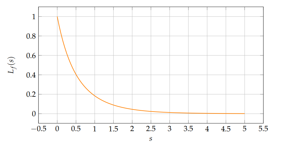
Theorem 8. If \(X\) is a Gompertz distribution, i.e. \(X\rightsquigarrow\mathcal{G}_z(b,\nu)\), with density \(f(x)=b\nu\exp(\nu + bx – \nu e^{bx})\mathbf{l}_{\{x>0\}}\),\(\; b,\nu > 0,\) then we have \[L_f(s)=\nu^{\displaystyle\frac{s}{b}}e^\nu\Gamma\left(1-\frac{s}{b}, \log(\nu)\right)\quad\forall\,b\geqslant s. \tag{23}\]
Proof. \[\begin{aligned} L_f(s)=&\displaystyle\int_0^{+\infty}b\nu\exp(\nu + bx – \nu e^{bx})e^{-sx}dx,\\ =&b\nu e^\nu\displaystyle\int_0^{+\infty}\exp\left((b-s)x – \nu e^{bx}\right),\\ =&\nu e^\nu\displaystyle\int_{\log(\nu)}^{+\infty}\exp\left(\left(1 – \frac{s}{b}\right)(t -\log(\nu)) – e^t \right)dt\;\text{where}\; t=bx + \log(\nu),\\ =&\nu^{\displaystyle\frac{s}{b}}e^\nu \int_{\log(\nu)}^{+\infty}\exp\left(\left(1 – \frac{s}{b}\right)t – e^t \right)dt. \end{aligned}\] The last formula of Proposition 4 completes this proof. ◻
Let \(\nu=1\), \(b=0.5\). Figure 4 shows \(L_f(s)\) computed via numerical integration.
Theorem 9. If \(X\) is a Inverse Gamma
distribution, i.e. \(X\rightsquigarrow\mathcal{IG}(\alpha,\beta)\),
with density
\(f(x)=\displaystyle\frac{\beta^\alpha}{\Gamma(\alpha)}x^{-\alpha
– 1}\exp\left(-\frac{\beta}{x}\right)\mathbf{l}_{\{x>0\}}, \;
\alpha,\beta > 0,\) then we have \[L_f(s)=2\displaystyle\frac{(\beta
s)^{\frac{\alpha}{2}}K_\alpha\left(2(\beta
s)^\frac{1}{2}\right)}{\Gamma(\alpha)}, \tag{24}\] where \(K_\nu\) is modified Bessel function of the
second kind (see Gradshteyn and Ryzhik [12]).
Proof. \[\begin{aligned} L_f(s)=&\displaystyle\frac{\beta^\alpha}{\Gamma(\alpha)}\int_0^{+\infty}\frac{1}{x^{\alpha + 1}}\exp\left(-sx – \frac{\beta}{x}\right)dx,\\ =&\displaystyle\frac{(s\beta)^\alpha}{\Gamma(\alpha)}\int_0^{+\infty}\frac{1}{u^{\alpha + 1}}\exp\left(-u-\frac{\beta s}{u}\right)du\;\text{where}\; u=sx,\\ =&\displaystyle\frac{2(\beta s)^\frac{\alpha}{2}}{\Gamma(\alpha)}\times\frac{1}{2}(\beta s)^\frac{\alpha}{2}\int_0^{+\infty}\frac{1}{u^{\alpha + 1}}\exp\left(-u-\frac{\beta s}{u}\right)du\\ =& \displaystyle\frac{2(\beta s)^\frac{\alpha}{2}}{\Gamma(\alpha)}K_\alpha(2\sqrt{\beta s})\;\text{where}\; K_\nu(z)=\displaystyle\frac{1}{2}\left(\frac{z}{2}\right)^\nu\int_0^{+\infty}\frac{e^{t – \frac{z^2}{t}}}{t^{\nu + 1}}dt\;\text{where}\,z\in\mathbb{R}_+^*. \end{aligned}\] ◻
Let \(\alpha=3\), \(\beta=2\). Figure 5 shows \(L_f(s)\) numerically.
Theorem 10. If \(X\) is a Normal distribution or Gaussian distribution, i.e. \(X\rightsquigarrow\mathcal{N}(\mu,\sigma^2)\), with density \(f(x)=\displaystyle\frac{1}{\sigma\sqrt{2\pi}}\exp\left(-\frac{1}{2}\left(\frac{x – \mu}{\sigma}\right)^2\right),\; \mu,\sigma > 0,\) then we obtain \[L_f(s)=\left[1 – \Phi(s\sigma)\right]\exp\left(-s\mu + \frac{\sigma^2 s^2}{2} \right), \tag{25}\] where \(\Phi\) is the cumulative distribution function of the standard normal distribution.
Proof. If \(Z\) is a standard normal deviate, then \(X=\sigma Z+\mu\) and \(\phi(x)=\displaystyle\frac{1}{\sqrt{2\pi}}\exp\left(-\frac{x^2}{2}\right)\) is the probability density function of the random variable \(Z\). We get \[\begin{aligned} L_\phi(s)=&\displaystyle\frac{1}{\sqrt{2\pi}}\int_0^{+\infty}\exp\left(-\frac{x^2}{2}\right)e^{-sx}dx,\\ =&\displaystyle\frac{e^{\frac{s^2}{2}}}{\sqrt{2\pi}}\int_0^{+\infty}\exp\left(-\frac{(x + s)^2}{2}\right)dx,\\ =&e^{\frac{s^2}{2}}\frac{1}{\sqrt{2\pi}}\int_s^{+\infty}\exp\left(-\frac{u^2}{2}\right)dx,\\ =& e^{\frac{s^2}{2}}\left[1 – \Phi(s)\right]. \end{aligned}\]
Moreover, we have \[\begin{aligned} L_f(s)=&\mathbb{E}\left[e^{-sX}\right]=\mathbb{E}\left[e^{-s(\sigma Z+ \mu)}\right]=e^{-s\mu}\mathbb{E}\left[e^{-(s\sigma)Z}\right]=L_\phi(s\sigma),\\ =&e^{-s\mu}\exp\left(\frac{(s\sigma)^2}{2}\right)\left[1 – \Phi(s\sigma)\right]. \end{aligned}\] ◻
Corollary 8. If \(X\) is a Log-Normal
distribution or Log-Gaussian distribution, i.e. \(X\rightsquigarrow\mathcal{LN}(\mu,\sigma^2)\),
with density
\(f(x)=\displaystyle\frac{1}{x\sigma\sqrt{2\pi}}\exp\left(-\frac{1}{2}\left(\frac{\log(x)
– \mu}{\sigma}\right)^2\right),\; \mu,\sigma > 0,\) then we
obtain \[L_f(s)=\displaystyle\sum_{n\geqslant
0}(-1)^n\Phi(n\sigma)\exp\left(n\mu + \frac{\sigma^2 n^2}{2}
\right)\frac{s^n}{n!}, \tag{26}\] where \(\Phi\) is the cumulative distribution
function of the standard normal distribution.
Proof. Suppose that, \(Y\) has a normal distribution, then the exponential function of \(Y\), \(X=\exp(Y)\), has a log-normal distribution. Thus, we have \(M^{(n)}_X(0)=\mathbb{E}\left[X^n\right]=\mathbb{E}\left[e^{nY}\right]=M_Y(n)\). Moreover, we get \[M_X(s)=\displaystyle\sum_{n\geqslant 0}M^{(n)}_X(0)\frac{s^n}{n!}=\displaystyle\sum_{n\geqslant 0}M_Y(n) \frac{s^n}{n!}=\displaystyle\sum_{n\geqslant 0}L_f(-n)\frac{s^n}{n!}.\]
Theorem 10 helps us write this easily \[L_f(s)=M_X(-s)=\displaystyle\sum_{n\geqslant 0}(-1)^n\left[1 – \Phi(-n\sigma)\right]\exp\left(n\mu + \frac{\sigma^2 n^2}{2} \right)\frac{s^n}{n!}.\]
It suffices to notice that \(\Phi(-t)=1-\Phi(t),\;\forall\;t>0\), which leads to the end of this proof. ◻
Let \(\mu=0\), \(\sigma=1\). Figure 6 shows \(L_f(s)\) computed numerically.
Theorem 11. If \(X\) is a Inverse Gaussian
distribution or Wald distribution, i.e. \(X\rightsquigarrow\mathcal{IN}(\mu,\sigma^2)\),
with density
\(f(x)=\displaystyle\sqrt{\frac{\sigma}{2\pi
x^3}}\exp\left[-\frac{\sigma(x – \mu)^2}{2\mu^2
x}\right]\mathbf{l}_{\{x>0\}},\; \mu,\sigma > 0,\) then we
have \[L_f(s)=\exp\left[\frac{\sigma}{\mu}\left(1 –
\left(1 +
\frac{2\mu^2s}{\sigma}\right)^{\displaystyle\frac{1}{2}}\right)\right]. \tag{27}\]
Proof. \[\begin{aligned} L_f(s)=&\displaystyle\int_0^{+\infty}\sqrt{\frac{\sigma}{2\pi x^3}}\exp\left[-\frac{\sigma(x – \mu)^2}{2\mu^2 x}\right]e^{-sx}dx,\\ =&\displaystyle\int_0^{+\infty}\sqrt{\frac{\sigma}{2\pi x^3}}\exp\left[-sx -\frac{\sigma(x – \mu)^2}{2\mu^2 x}\right]dx,\\ =&\displaystyle\int_0^{+\infty}\sqrt{\frac{\sigma}{2\pi x^3}}\exp\left(\frac{\sigma}{\mu}\right)\exp\left[\frac{-\sigma}{2\mu^2 x}\left(\left(1 + \frac{2\mu^2 s}{\sigma}\right)x^2 + \mu^2\right)\right]dx,\\ =&\displaystyle\int_0^{+\infty}\sqrt{\frac{\sigma}{2\pi x^3}}\exp\left(\frac{\sigma}{\mu}\right)\exp\left[\frac{-\sigma}{2\mu^2 x}\left(\left(\sqrt{1 +\frac{2\mu^2 s}{\sigma}}x – \mu\right)^2 + 2\mu x\sqrt{1 +\frac{2\mu^2 s}{\sigma}}\right)\right]dx,\\ =&\exp\left[\frac{\sigma}{\mu}\left(1 – \sqrt{1 +\frac{2\mu^2 s}{\sigma}}\right)\right]\displaystyle\int_0^{+\infty}\sqrt{\frac{\sigma}{2\pi x^3}}\exp\left[\frac{-\sigma}{2\mu^2 x}\left(\sqrt{1 +\frac{2\mu^2 s}{\sigma}}x – \mu\right)^2\right]dx,\\ =&\exp\left[\frac{\sigma}{\mu}\left(1 – \sqrt{1 +\frac{2\mu^2 s}{\sigma}}\right)\right]\displaystyle\int_0^{+\infty}\sqrt{\frac{\sigma}{2\pi x^3}}\exp\left[\frac{-\sigma}{2\left(\displaystyle\frac{\mu}{\sqrt{1 +\frac{2\mu^2 s}{\sigma}}}\right)^2 x}\left(x – \frac{\mu}{\sqrt{1 +\frac{2\mu^2 s}{\sigma}}}\right)^2\right]dx,\\ =&\exp\left[\frac{\sigma}{\mu}\left(1 – \sqrt{1 +\frac{2\mu^2 s}{\sigma}}\right)\right],\\ \end{aligned}\] because \[\displaystyle\int_0^{+\infty}\sqrt{\frac{\sigma}{2\pi x^3}}\exp\left[\frac{-\sigma}{2\left(\displaystyle\frac{\mu}{\sqrt{1 +\frac{2\mu^2 s}{\sigma}}}\right)^2 x}\left(x – \frac{\mu}{\sqrt{1 +\frac{2\mu^2 s}{\sigma}}}\right)^2\right]dx=\displaystyle\int_0^{+\infty}\displaystyle\sqrt{\frac{\sigma}{2\pi x^3}}\exp\left[-\frac{\sigma(x – \mu_s)^2}{2\mu_s^2 x}\right] dx=1,\] where \(\mu_s=\displaystyle\frac{\mu}{\sqrt{1 +\frac{2\mu^2 s}{\sigma}}}\). ◻
Theorem 12. If \(X\) is a Student distribution, i.e. \(X\rightsquigarrow\mathcal{T}(\nu)\), with density \(f(x)=\displaystyle\frac{1}{\sqrt{\nu}B\left(\frac{\nu}{2},\frac{1}{2}\right)}\left(1 + \frac{x^2}{\nu}\right)^{-\frac{\nu + 1}{2}},\;\\ \nu > 0,\) then we have \[L_f(s)=\displaystyle\frac{\nu + 1}{2}\sum_{n\geqslant 0}(-1)^{n + 1}\frac{s^{n-1}}{n!}\nu^{\frac{n – 1}{2}}\frac{ B\left(\frac{n}{2} + 1,\frac{\nu – n + 1}{2}\right)}{B\left(\frac{\nu}{2},\frac{1}{2}\right)}, \tag{28}\] where \(B\) is the Beta function.
Proof. A direct consequence of Corollary 1 is \(L_\psi(s)=sL_f(s)\) where \(\displaystyle\frac{d}{d x}f(x)=\psi(x)\). We obtain, \(\psi(x)=-\displaystyle\frac{n + 1}{n}\frac{1}{\sqrt{\nu}B\left(\frac{\nu}{2},\frac{1}{2}\right)}\frac{x}{\left(1 + \frac{x^2}{\nu}\right)^{\frac{n + 3}{2}}}\) and by the Taylor series representation, we write \[\begin{aligned} L_\psi(s)=&-\displaystyle\frac{n + 1}{n}\frac{1}{\sqrt{\nu}B\left(\frac{\nu}{2},\frac{1}{2}\right)}\int_0^{+\infty}\frac{x}{\left(1 + \frac{x^2}{\nu}\right)^{\frac{n + 3}{2}}}e^{-sx}dx,\\ =&-\displaystyle\frac{n + 1}{n}\frac{1}{\sqrt{\nu}B\left(\frac{\nu}{2},\frac{1}{2}\right)}\sum_{n\geqslant 0}(-1)^n\frac{s^n}{n!}\int_0^{+\infty}\frac{x^{n+1}}{\left(1 + \frac{x^2}{\nu}\right)^{\frac{n + 3}{2}}}dx,\\ =&\displaystyle\frac{n + 1}{2}\frac{1}{B\left(\frac{\nu}{2},\frac{1}{2}\right)}\sum_{n\geqslant 0}(-1)^{n + 1}\nu^{\frac{n-1}{2}}\frac{s^n}{n!}\int_0^{+\infty}\frac{u^{\frac{n}{2}}}{(u+1)^{\frac{n+3}{2}}}du,\quad\text{where}\;x^2=\nu u,\\ =&\displaystyle\frac{n + 1}{2}\frac{1}{B\left(\frac{\nu}{2},\frac{1}{2}\right)}\sum_{n\geqslant 0}(-1)^{n + 1}\nu^{\frac{n-1}{2}}\frac{s^n}{n!}B\left(\frac{n}{2} + 1, \frac{\nu – n + 1}{2}\right). \end{aligned}\]
Finally, to complete this proof, it suffices to notice that \(L_f(s)=\displaystyle\frac{1}{s}L_\psi(s)\). ◻
Theorem 13. If \(X\) is a Laplace distribution, i.e. \(X\rightsquigarrow\mathcal{L}_p(\mu,b)\), with density \(f(x)=\displaystyle\exp\left(-\frac{|x – \mu|}{b}\right),\\ \;\forall \mu,b> 0,\) then we have
\[L_f(s)= \left\{\begin{array}{ll} \displaystyle\frac{\exp\left(\frac{\mu}{b}\right)}{2(1 + bs)},\quad\text{if}\;\mu\leqslant 0,\\ \displaystyle\frac{2\exp(-s\mu) – (1 + bs)\exp\left(-\frac{\mu}{b}\right)}{1 – b^2s^2},\quad\text{if}\;\mu>0\;\text{and}\; s<\displaystyle\frac{1}{b}. \end{array}\right.\]
Proof. \[\begin{aligned} L_f(s)=&\displaystyle\int_0^{+\infty}\exp\left(-\frac{|x – \mu|}{b}\right)e^{-sx}dx,\\ =&\displaystyle\int_0^{+\infty}\exp\left(-sx – \frac{|x – \mu|}{b}\right)dx,\\ =&\displaystyle\frac{e^{-s\mu}}{2}\int_{\frac{-\mu}{b}}^{+\infty}\exp(-|t| – sbt)dt,\\ \end{aligned}\]
\(\triangleright\) For \(\mu\leqslant 0\), then \(\displaystyle\frac{-\mu}{b}\geqslant 0\) and we have \[\begin{aligned} L_f(s)=&\displaystyle\frac{e^{-s\mu}}{2}\int_{\frac{-\mu}{b}}^{+\infty}\exp[-(1 + s b)t]dt,\\ =&\displaystyle\frac{\exp\left(\frac{\mu}{b}\right)}{2(1 + bs)}. \end{aligned}\]
\(\triangleright\) For \(\mu>0\), then \(\displaystyle\frac{-\mu}{b}< 0\) and we have with \(sb<1\), \[\begin{aligned} L_f(s)=&\displaystyle\frac{e^{-s \mu}}{2}\left[\int_{\frac{-\mu}{b}}^{0}\exp[(1 – sb)t]dt + \int_{\frac{-\mu}{b}}^{+\infty}\exp[-(1 + sb)t]dt \right],\\ =&\displaystyle\frac{e^{-s \mu}}{2}\left[\frac{1 – \exp\left(-\frac{\mu}{b} + s\mu\right)}{1 – sb} + \frac{1}{1 + sb} \right],\\ =&\displaystyle\frac{2\exp(-s\mu) – (1 + bs)\exp\left(-\frac{\mu}{b}\right)}{1 – b^2s^2}. \end{aligned}\] ◻
It is important to emphasize that reliability is a key measure of the probability that an element will satisfactorily perform its designed function over a given time interval and under specific conditions. In the field of reliability, the concept of system availability, symbolized by \(D(t)\), corresponds to the probability that the system is operational at a given time \(t\) (see Barlow et al. [4]).
Consider that at the initial time \(t = 0\), a new device is commissioned and operates for a duration \(X_1\), which marks the time of its first failure. The duration of the first repair is denoted \(Y_1\). Therefore, the device restarts at time \(X_1 + Y_1\), followed by a new operating period of duration \(X_2\). We assume that operating times obey the same statistical distribution, as do repair times. Thus, we have two sequences of random variables, denoted respectively \((X_n)_{n \geqslant 0}\) and \((Y_n)_{n \geqslant 0}\), which are independent and identically distributed, with respective probability densities \(f\) and \(g\), and independent of each other. These sequences successively model the operating times and the repair times. In this theoretical framework, the nth restart of the system occurs at time \(X_1 + Y_1 + \cdots + X_n + Y_n\). Thus, the restart counting process is similar to a renewal process; we even speak of alternating renewal, because the operating periods alternate with the repair periods.
The following theorem will provide a description of the asymptotic availability of a system, and its demonstration is based on the use of the Laplace transform of probability distributions.
Theorem 14. In an alternating renewal process, let us denote \(\mu_X\) and \(\mu_Y\) the respective expectations of \(X_n\) and \(Y_n\) and \(D(t)\) the availability at the time \(t\geqslant 0\). The asymptotic availability is given by: \[\label{Dt} D(t)\stackrel{t\rightarrow +\infty}{\longrightarrow} D_{\infty}=\displaystyle\frac{\mu_X}{\mu_X + \mu_Y}\,. \tag{29}\]
Proof. If there are been exactly \(n\) restarts before time \(t\), the system works if \(t\) is between the time of the nth restart and that of the \((n + 1)-\)th breakdown. Let \(T_0=0\) and for \(n\in \mathbb{N}^*\), \[T_n = X_1 + Y_1 +\cdots + X_n + Y_n \quad \text{and}\quad M_n = T_{n-1} + X_n.\]
Therefore, we can write \[\begin{aligned} D(t) =& \displaystyle\sum_{n\geqslant 0}\mathbb{P}[T_n\leqslant t < M_{n+1}]\\ =& \displaystyle\sum_{n\geqslant 0}(\mathbb{P}[T_n\leqslant t ] – \mathbb{P}[M_{n+1}\leqslant t ])\\ =& \displaystyle\sum_{n\geqslant 0}[H_n(t) – Q_n(t)],\\ \end{aligned}\] where \(H_n\) and \(Q_n\) are the respective distribution functions of \(T_n\) and \(M_{n+1}\). Let \(h_n\) and \(q_n\) denote their probability density functions. By applying the Corollary 2 to the probability densities of the sequences of random variables \(T_n\) and \(M_{n+1}\), we have: \[\label{hq} L_{h_n}(s)=\left(L_f(s)L_g(s)\right)^n\quad\text{and}\quad L_{q_n}(s)=L_f(s)\left(L_f(s)L_g(s)\right)^n. \tag{30}\]
We obtain the Laplace transforms of the distribution functions \(H_n\) and \(Q_n\) thanks to Corollary 1, by dividing the expressions of(30) by \(s\). Using the linearity of the Laplace transform, we determine the Laplace transform of D(t) by writing: \[\begin{aligned} L_D(s) =& \displaystyle\sum_{n\geqslant 0}\left[\displaystyle\frac{1}{s}\left(L_f(s)L_g(s)\right)^n – \displaystyle\frac{1}{s}L_f(s)\left(L_f(s)L_g(s)\right)^n\right] \\ =& \displaystyle\frac{1}{s}[1 – L_f(s)]\displaystyle\sum_{n\geqslant 0} \left(L_f(s)L_g(s)\right)^n \\ =& \displaystyle\frac{1 – L_f(s)}{s(1 – L_f(s)L_g(s))}. \end{aligned}\]
The Taylor expansion to order 1 of \(L_f(s)\) and \(L_g(s)\) in the neighborhood of \(s=0\) gives respectively \[\label{DL} L_f(s)=1 – \mu_Xs + o(s)\quad\text{and}\quad L_g(s)=1 – \mu_Ys + o(s). \tag{31}\]
Furthermore, we know that if the function \(D(t)\) admits a limit in \(+\infty\), \(sL_D(s)\) also admits a limit in \(0\) and they are equal. Thus, we have \[\label{LimitfLF} \lim_{t\longrightarrow +\infty}D(t)=\lim_{s\longrightarrow 0}sL_D(s). \tag{32}\]
The equalities (31) and (32) complete the proof of this theorem. ◻
The result of Theorem 14 is quite predictable since the operating periods, which last on average \(\mu_X\), alternate with the repair periods, which last \(\mu_Y\). In the long term, the probabilities of finding the device working or broken are proportional to \(\mu_X\) and \(\mu_Y\). So, we have \[\displaystyle\frac{D(t)}{\mu_X} \approx \displaystyle\frac{1 – D(t)}{\mu_Y} \Longleftrightarrow D_{\infty}=\displaystyle\frac{\mu_X}{\mu_X + \mu_Y}.\]
Consider a series system with two components, lifetimes \(X_1\sim \mathcal{E}(1)\) and \(X_2\sim \Gamma(2,1)\). The system reliability: \[R_{\text{sys}}(t) = \mathbb{P}(X_1>t)\cdot \mathbb{P}(X_2>t).\]
Laplace transform: \[L_{R_{\text{sys}}}(s) = L_{X_1}(s) \cdot L_{X_2}(s) = \frac{1}{1+s} \cdot \left(\frac{1}{1+s}\right)^2 = \frac{1}{(1+s)^3}.\]
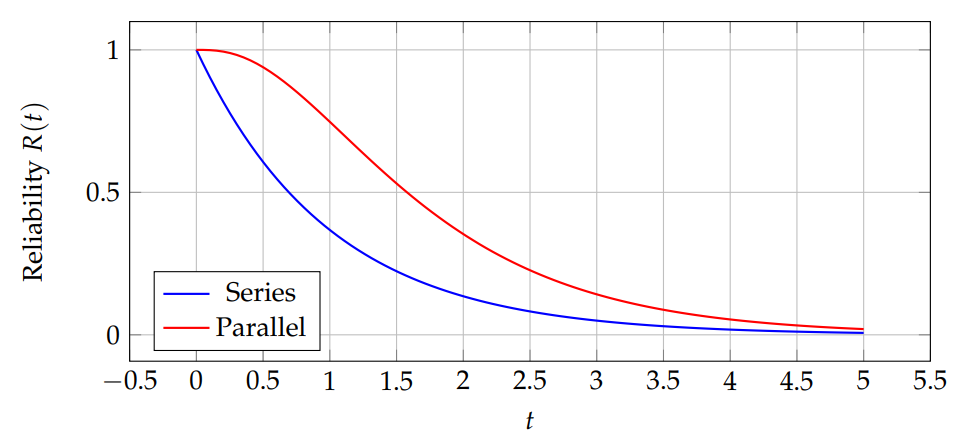
\(\circ\) Series system: system fails if any component fails. \[R_{series}(t) = \prod_{i=1}^n R_i(t) = \prod_{i=1}^n \Pr(X_i > t).\]
\(\circ\) Parallel system: system fails if all components fail. \[R_{parallel}(t) = 1 – \prod_{i=1}^n (1-R_i(t)).\]
Assume 3 components with Log-Normal, Gompertz, and Pareto lifetimes. Compute \(R_{series}(t)\) and \(R_{parallel}(t)\) numerically using the Laplace transforms. Figures 7 shows series vs parallel reliability curves.
Expected uptime before scheduled maintenance at \(T\): \[U(T) = \int_0^T \mathbb{P}(X>t) dt, \quad L[U(T)](s) = \frac{1-e^{-sT}}{s} L_f(s).\]
Remark 2. Note that the Laplace transforms is also used to evaluate expected lifetime of components and to optimize preventive maintenance intervals based on \(E[T] = -dL_f(s)/ds|_{s=0}\).
In this article, we have highlighted some fundamental properties of the Laplace transform as it relates to probability theory, highlighting its distinctive characteristics compared to commonly encountered probability distributions. We have also established various results concerning the application of the Laplace transform to well-known probability densities, which have proven to be particularly complex. These results have significant implications in the field of reliability, particularly with regard to determining system availability using this tool.
Indeed, they open the way to promising prospects for the search for analytical solutions to various problems, such as those associated with partial differential equations, integro-differential equations, Navier-Stokes equations, and stochastic processes. Furthermore, the Laplace transform has proven to be a valuable tool for identifying sub-Gaussian random variables, thus facilitating the study of their convergence within an Orlicz space.
In light of the work carried out in this article, we also plan to direct our future research toward the z-transform, an essential mathematical tool in the fields of automation and signal processing. This transform, the discrete equivalent of the Laplace transform, allows the conversion of a real signal in the time domain into a complex series. This field of study thus promises rich prospects for our future research.