
This paper is an introduction to the mathematics of quantum physics and quantum computation. The emphasis is put on the basic mathematical aspects of definitions and operations on qubits. Following [1– 3], we start by a comprehensive introduction of a qubit. A qubit is the fundamental quantum state representing the smallest unit of quantum information containing one bit of classical information accessible by measurement. It is represented by or identified to a state vector which is a unit element of \(\mathbb{C}^2\). We describe its representations on unit spheres in \(\mathbb{R}^3\). These representations lead to the interpretation of Pauli operators as basic rotations in \(\mathbb{R}^3\). Then we study unitary operators, and their link to rotations in \(\mathbb{R}^3\) is established using the density operator associated to a qubit. We obtain quite easily the expressions for the composition and the non-commutativity of two rotations. We complete this paper by some decomposition, or splitting, problems of unitary operators on \(\mathbb{C}^2\) obtained from results on rotations in \(\mathbb{R}^3\) [4, 5]. This last subject is related to gates in quantum computation [6].
Throughout this paper we use the Dirac bracket notation for elements of the two-dimensional complex vector space \(\mathbb{C}^2\) generated by two vectors \[\mathbb{C}^2 = \mathrm{Lin}\left\{ | 0 \rangle, | 1 \rangle \right\} = \left\{ \; | q \rangle = a | 0 \rangle + b | 1 \rangle \; : \; a, b \in \mathbb{C} \; \right\}.\]
For \(| q_l \rangle = a_l | 0 \rangle + b_l |1 \rangle\) \((l = 1,2)\) we use the Hermitian inner product \[\langle q_1 | q_2\rangle = a_1^*a_2 \langle 0 | 0 \rangle + a_1^*b_2 \langle 0 | 1 \rangle + b_1^*a_2 \langle 1 | 0 \rangle + b_1^*b_2 \langle 1 | 1 \rangle.\]
We suppose that \[\langle i | j \rangle = \delta_{ij} = \left\{\begin{array}{ccc} 1 & \text{ if } & i=j \\ 0 & \text{ if } & i \neq j \end{array}\right. \quad \text{for} \quad i,j \in \left\{0,1\right\},\] so that the set \(\left\{ |0\rangle, |1\rangle \right\}\) is an orthonormal basis for \(\mathbb{C}^2\). We get \[\langle q_1 | q_2 \rangle = a_1^*a_2 + b_1^*b_2 ,\] and the length of \(|q\rangle\) is \(\left\| |q\rangle \right\| = \sqrt{ \langle q | q \rangle } = \sqrt{ \left|a\right|^2 + \left|b\right|^2}\). A good introduction to the mathematics of finite-dimensional complex vector spaces is [7].
A qubit is any unit length element of \(\mathbb{C}^2\). It can be written as \[| q \rangle = e^{i\psi} \left[ \cos\left( \theta/2 \right) |0\rangle + \sin\left( \theta/2 \right) e^{i\varphi} |1\rangle \right]\] for \(\theta \in \left[0,\pi\right]\), \(\varphi \in \left[0,2\pi\right)\), and \(\psi \in \mathbb{R}\). We will identify qubit up to its phase \(e^{i\psi}\), i.e. \[| q \rangle \equiv | q' \rangle \quad \text{iff} \quad \exists_{\psi\in\mathbb{R}} \ | q' \rangle = e^{i\psi}| q \rangle,\] so qubits are equivalence classes of unit length elements of \(\mathbb{C}^2\). We will use \[| q \rangle = \cos\left(\theta/2\right) |0\rangle + \sin\left(\theta/2\right) e^{i\varphi} |1\rangle ,\] as its representative.
A qubit \(| q^{\bot} \rangle\), orthogonal to the qubit \(| q \rangle\), is given by \[| q^{\bot} \rangle = \cos\left(\frac{\pi-\theta}{2}\right) | 0 \rangle + \sin\left(\frac{\pi-\theta}{2}\right) e^{i(\pi+\varphi)} | 1 \rangle ,\] so that \(\langle q | q^{\bot} \rangle = 0\).
We can represent qubits on the upper-half unit sphere in \(\mathbb{R}^3\). Each qubit \(| q \rangle\) with \(\theta \in \left[0,\pi\right)\) is represented by a unique point, while for \(\theta = \pi\), \(| q \rangle = e^{i\varphi} |1\rangle \equiv |1\rangle\) is represented by the whole unit circle \(x^2+y^2=1\) and \(z=0\).
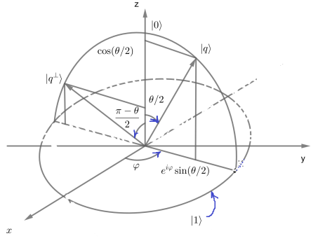
For example, \(| q \rangle\) and \(| q^{\bot}\rangle\) are indicated on Figure 1. Their corresponding vectors are \[\left\{ \begin{array}{ccl} x =& \sin\left( \frac{\theta}{2} \right)\cos(\varphi) , \\ y =& \sin\left( \frac{\theta}{2} \right)\sin(\varphi) , \\ z =& \cos\left( \frac{\theta}{2} \right) , \end{array}\right. \quad \text{and} \quad \left\{ \begin{array}{ccl} x^{\bot} =& \sin\left(\frac{\pi-\theta}{2}\right)\cos(\pi+\varphi) , \\ y^{\bot} =& \sin\left(\frac{\pi-\theta}{2}\right)\sin(\pi+\varphi) , \\ z^{\bot} =& \cos\left(\frac{\pi-\theta}{2}\right). \end{array}\right.\]
To obtain only one point on the sphere for \(|1\rangle\), we continuously transform the point \((x,y,z)\) as follows \[\left\{ \begin{array}{ccl} x_{\lambda} =& \sin\left( \frac{1+\lambda }{2} \theta \right)\cos(\varphi) , \\ y_{\lambda} =& \sin\left( \frac{1+\lambda }{2} \theta \right)\sin(\varphi) , \\ z_{\lambda} =& \cos\left( \frac{1+\lambda }{2} \theta \right) , \end{array}\right. \quad \text{for} \quad \lambda \in \left[0,1\right].\]
At the end of the transformation, for \(\lambda = 1\), we get \[\left\{ \begin{array}{lcl} x_{1} =& \sin\left( \theta \right)\cos(\varphi) , \\ y_{1} =& \sin\left( \theta \right)\sin(\varphi) , \\ z_{1} =& \cos\left( \theta \right). \end{array}\right.\]
Hence the qubit \(| q \rangle = \cos\left( \frac{\theta}{2} \right) |0\rangle + \sin\left( \frac{\theta}{2} \right) e^{i\varphi} |1\rangle\) is represented by the vector \[\vec{q} = \left( \sin\left( \theta \right)\cos(\varphi) , \sin\left( \theta \right)\sin(\varphi) , \cos\left( \theta \right) \right),\] on the unit sphere of \(\mathbb{R}^3\). On the same way, for \(| q^{\bot} \rangle\) we get \[\begin{aligned} \vec{q}^{\bot} =& \left( \sin\left( \pi-\theta \right)\cos(\pi+\varphi) , \sin\left( \pi-\theta \right)\sin(\pi+\varphi) , \cos\left( \pi -\theta \right) \right) \\ =& -\left( \sin\left( \theta \right)\cos(\varphi) , \sin\left( \theta \right)\sin(\varphi) , \cos\left( \theta \right) \right) \\ =&- \vec{q}. \end{aligned}\]
This representation on the unit sphere of \(\mathbb{R}^3\) is called the Bloch sphere representation of a qubit (see Figure 2), and we have the next result.
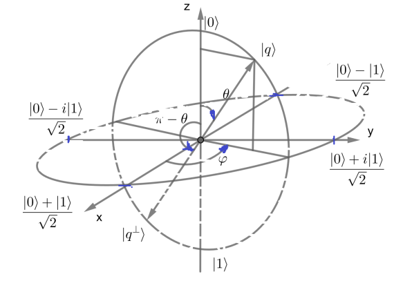
Theorem 1. The correspondence \(| q \rangle \leftrightarrow \vec{q}\) is a bijection.
The spherical representation for qubits in \(\mathbb{R}^3\) suggests to take a look at rotations in \(\mathbb{R}^3\). Let us start by considering rotations around the axis \(OX\), \(OY\), and \(OZ\). More general rotations will be considered later in this text.
The rotation of an angle \(\xi\) around the vector \(\vec{i}\) is given by \[R_{(\vec{i},\xi)} = \left[ \begin{array}{rrr} 1 & 0 & 0 \\ 0 & \cos(\xi) & -\sin(\xi) \\ 0 & \sin(\xi) & \cos(\xi) \end{array} \right],\] and for \(\xi = \pi\) we get \[\vec{q}\;' = R_{(\vec{i},\pi)}(\vec{q}) = \left( \begin{array}{l} \sin\left(\pi-\theta\right)\cos\left(-\varphi\right) \\ \sin\left(\pi-\theta\right)\sin\left(-\varphi\right) \\ \cos\left(\pi-\theta\right) \end{array} \right).\]
So the corresponding qubit is \[\begin{aligned} | q' \rangle =& \cos\left(\frac{\pi-\theta}{2}\right) | 0 \rangle + \sin\left(\frac{\pi-\theta}{2}\right)e^{-i\varphi} | 1 \rangle \\ =& e^{-i\varphi} \left[ \cos\left(\theta/2\right) | 1 \rangle + \sin\left(\theta/2 \right) e^{i\varphi} | 0 \rangle \right]. \end{aligned}\]
If we set \(\hat{\sigma}_x | 0 \rangle = | 1 \rangle\) and \(\hat{\sigma}_x | 1 \rangle = | 0 \rangle\), we get \(| q' \rangle = e^{-i\varphi} \hat{\sigma}_x | q \rangle \equiv \hat{\sigma}_x | q \rangle\).
For the rotation around the vector \(\vec{j}\) we have \[R_{(\vec{j},\xi)} = \left[ \begin{array}{rrr} \cos(\xi) & 0 & \sin(\xi) \\ 0 & 1 & 0 \\ -\sin(\xi) & 0 & \cos(\xi) \end{array} \right].\]
For \(\xi = \pi\) we get \[\vec{q}\;' = R_{(\vec{j},\pi)}(\vec{q}) = \left( \begin{array}{l} \sin\left(\pi-\theta\right)\cos\left(\pi-\varphi\right) \\ \sin\left(\pi-\theta\right)\sin\left(\pi-\varphi\right) \\ \cos\left(\pi-\theta\right) \end{array}\right),\] hence \[\begin{aligned} | q' \rangle =& \cos\left(\frac{\pi-\theta}{2}\right) | 0 \rangle + \sin\left(\frac{\pi-\theta}{2}\right)e^{i(\pi-\varphi)} | 1 \rangle \\ =& e^{i(\frac{\pi}{2}-\varphi)} \left[ \cos\left(\theta/2\right) i | 1 \rangle + \sin\left(\theta/2 \right) e^{i\varphi} (-i) | 0 \rangle \right]. \end{aligned}\]
If we set \(\hat{\sigma}_y | 0 \rangle = i | 1 \rangle\) and \(\hat{\sigma}_y | 1 \rangle = -i | 0 \rangle\), we get \(| q' \rangle = e^{i(\frac{\pi}{2}-\varphi)} \hat{\sigma}_y | q \rangle \equiv \hat{\sigma}_y | q \rangle\).
For the rotation around the vector \(\vec{k}\) we have \[R_{(\vec{k},\xi)} = \left[ \begin{array}{rrr} \cos(\xi) & -\sin(\xi) & 0 \\ \sin(\xi) & \cos(\xi) & 0 \\ 0 & 0 & 1 \end{array} \right],\] so \[\vec{q}\;' = R_{(\vec{k},\pi)} (\vec{q}) = \left( \begin{array}{l} \sin\left(\theta\right)\cos\left(\pi+\varphi\right) \\ \sin\left(\theta\right)\sin\left(\pi+\varphi\right) \\ \cos\left(\theta\right) \end{array}\right),\] and \[\begin{aligned} | q' \rangle =& \cos\left(\theta/2\right) | 0 \rangle + \sin\left(\theta/2\right)e^{i(\pi+\varphi}| 1 \rangle \\ =& \cos\left(\theta/2\right) | 0 \rangle + \sin\left(\theta/2 \right) e^{i\varphi} (-1) | 1 \rangle. \end{aligned}\]
If we set \(\hat{\sigma}_z | 0 \rangle = | 0 \rangle\) and \(\hat{\sigma}_z | 1 \rangle = – | 1 \rangle\), we get \(| q' \rangle = \hat{\sigma}_z | q \rangle\).
The linear operators \(\hat{\sigma}_x\), \(\hat{\sigma}_y\), and \(\hat{\sigma}_z\) defined above form the set of Pauli operators on \(\mathbb{C}^2\). They correspond to half-revolutions in \(\mathbb{R}^3\).
Let \(\hat{A} : \mathbb{C}^2 \rightarrow \mathbb{C}^2\) be a linear operator. Its adjoint \(\hat{A}^+\) is defined by the relation \[\langle v | \hat{A}^+ | u \rangle = \langle v | ( \hat{A}^+ | u \rangle ) \rangle = \langle u | ( \hat{A} | v \rangle ) \rangle^* = \langle u | \hat{A} | v \rangle^*,\] for all \(| u \rangle , | v \rangle \in \mathbb{C}^2\). It is easy to observe that \(( \hat{B} \hat{A} )^+ = \hat{A}^+ \hat{B}^+\). We say that \(\hat{A}\) is a positive linear operator iff (if and only if) \(\langle u | \hat{A} | u \rangle \geq 0\) for all \(| u \rangle \in \mathbb{C}^2\).
Let us consider the following definitions:
\(\hat{A}\) is a normal operator iff \(\hat{A}\hat{A}^+ = \hat{A}^+\hat{A}\);
\(\hat{A}\) is a unitary operator iff \(\hat{A}^+ = \hat{A}^{-1}\);
\(\hat{A}\) is a Hermitian operator iff \(\hat{A}^+ = \hat{A}\).
Obviously, any unitary or Hermitian operator is also a normal operator.
For \(| q \rangle \in \mathbb{C}^2\), we define the external product \(| q \rangle\langle q|\) (also known as a projection operator) which is a positive Hermitian linear operator. Indeed
positive: because \(\langle p | q \rangle \langle q | p \rangle = |\langle q | p \rangle |^2\geq 0\);
Hermitian (and hence normal) because \(\left( | q \rangle \langle q | \right)^+ = | q \rangle \langle q |\).
We also observe that \[\left( | q \rangle \langle q | \right)^k = \left\| q \right\|^{2(k-1)} | q \rangle \langle q | ,\] for \(k=1,2,3,…\)
For any orthonormal basis \(\left\{ | v_0 \rangle, | v_1 \rangle \right\}\) of \(\mathbb{C}^2\), we get the identity operator, noted \(\hat{\sigma}_o\), from \[\hat{\sigma}_o = | v_0 \rangle \langle v_0 | + | v_1 \rangle \langle v_1 |.\]
Also, using any orthonormal basis \(\left\{ | v_0 \rangle, | v_1 \rangle \right\}\) of \(\mathbb{C}^2\), the trace of a linear operator is given by \[\mathrm{Tr}(\hat{A}) = \langle v_0 | \hat{A} | v_0 \rangle + \langle v_1 | \hat{A} | v_1 \rangle,\] and this value does not depend on the choice of the orthonormal basis used for the computation.
For two vectors \(\vec{u}\) and
\(\vec{v}\) of \(\mathbb{R}^3\), the dot and cross products
are respectively noted by \(\vec{u} \cdot
\vec{v}\) and \(\vec{u} \times
\vec{v}\). We recall here standard results about dot and cross
products which will used in the next sections. Proofs of these results
can be found for example in [8, 9].
Lemma 1. Let \(\vec{a}\), \(\vec{b}\), \(\vec{c}\), and \(\vec{d}\) in \(\mathbb{R}^3\). We have
\((\vec{a} \times \vec{b}) = – (\vec{b} \times \vec{a})\) ;
\(\vec{a} \cdot (\vec{b} \times \vec{c}) = \vec{c}\cdot(\vec{a} \times \vec{b}) = \vec{b}\cdot(\vec{c} \times \vec{a})\) ;
\(\vec{a} \times (\vec{b} \times \vec{c}) = (\vec{a}\cdot\vec{c}) \vec{b} – (\vec{a}\cdot\vec{b}) \vec{c}\) ;
\((\vec{a} \times \vec{b}) \cdot (\vec{c} \times \vec{d}) = (\vec{a}\cdot\vec{c})(\vec{b}\cdot\vec{d}) – (\vec{b}\cdot\vec{c})(\vec{a}\cdot\vec{d})\);
\(\vec{d} \cdot \big(\vec{a} \times (\vec{b} \times \vec{c})\big) = (\vec{d} \times \vec{a}) \cdot (\vec{b} \times \vec{c})\).
The set \(\mathcal{S} = \left\{\hat{\sigma}_o,\hat{\sigma}_x,\hat{\sigma}_y,\hat{\sigma}_z\right\}\) form a basis of the \(4\)-dimensional vector space of linear operators on \(\mathbb{C}^2\). Table 1 presents the composition table for the \(4\) elements of this basis.
| \(\hat{\sigma}_o\) | \(\hat{\sigma}_x\) | \(\hat{\sigma}_y\) | \(\hat{\sigma}_z\) | |
|---|---|---|---|---|
| \(\hat{\sigma}_o\) | \(\hat{\sigma}_o\) | \(\hat{\sigma}_x\) | \(\hat{\sigma}_y\) | \(\hat{\sigma}_z\) |
| \(\hat{\sigma}_x\) | \(\hat{\sigma}_x\) | \(\hat{\sigma}_o\) | \(i \hat{\sigma}_z\) | \(-i \hat{\sigma}_y\) |
| \(\hat{\sigma}_y\) | \(\hat{\sigma}_y\) | \(-i \hat{\sigma}_z\) | \(\hat{\sigma}_o\) | \(i \hat{\sigma}_x\) |
| \(\hat{\sigma}_z\) | \(\hat{\sigma}_z\) | \(i \hat{\sigma}_y\) | \(-i \hat{\sigma}_x\) | \(\hat{\sigma}_o\) |
Proposition 1. The Pauli operators are unitary and Hermitien, and hence normal.
Let \(\vec{v} = \left( v_x, v_y, v_z \right) \in \mathbb{R}^3\) and \(\hat{\sigma} = \left( \hat{\sigma}_x , \hat{\sigma}_y ,\hat{\sigma}_z \right)\). We define the operator \[\vec{v} \cdot \hat{\sigma} = v_x \hat{\sigma}_x + v_y \hat{\sigma}_y + v_z \hat{\sigma}_z.\]
Next are some basic results useful for the next sections.
Proposition 2. For \(\vec{a}\) and \(\vec{b}\) in \(\mathbb{R}^3\) \[(\vec{a}\cdot\hat{\sigma}) (\vec{b}\cdot\hat{\sigma})= (\vec{a}\cdot\vec{b})\hat{\sigma}_o + i (\vec{a}\times\vec{b}) \cdot \hat{\sigma}.\]
Corollary 1. For \(\vec{n}\) in \(\mathbb{R}^3\), \((\vec{n}\cdot\hat{\sigma}) (\vec{n}\cdot\hat{\sigma}) = \left\|\vec{n}\right\|^2 \hat{\sigma}_o.\)
Corollary 2. For \(\vec{a}\) and \(\vec{b}\) in \(\mathbb{R}^3\)
\((\vec{a}\cdot\hat{\sigma}) (\vec{b}\cdot\hat{\sigma}) + (\vec{b}\cdot\hat{\sigma}) (\vec{a}\cdot\hat{\sigma}) = 2(\vec{a}\cdot\vec{b})\hat{\sigma}_o\),
\((\vec{a}\cdot\hat{\sigma}) (\vec{b}\cdot\hat{\sigma}) – (\vec{b}\cdot\hat{\sigma}) (\vec{a}\cdot\hat{\sigma}) = 2i (\vec{a}\times\vec{b}) \cdot \hat{\sigma}\).
Corollary 3. For \(\vec{a}\) and \(\vec{b}\) in \(\mathbb{R}^3\)
\((\vec{a}\cdot\hat{\sigma}) (\vec{b}\cdot\hat{\sigma}) (\vec{a}\cdot\hat{\sigma}) = – \left\|\vec{a} \right\|^2(\vec{b}\cdot\hat{\sigma}) + 2 (\vec{a} \cdot\vec{b}) (\vec{a}\cdot\hat{\sigma})\),
\((\vec{a}\cdot\hat{\sigma}) (\vec{b}\cdot\hat{\sigma}) (\vec{a}\cdot\hat{\sigma}) = \left\|\vec{a} \right\|^2(\vec{b}\cdot\hat{\sigma}) + 2i (\vec{a}\times\vec{b})\cdot \hat{\sigma} (\vec{a}\cdot\hat{\sigma})\).
Proposition 3. For the qubit \(| q \rangle \in \mathbb{C}^2\)
\(\vec{q}\cdot\hat{\sigma} | q \rangle = | q \rangle\),
\(\vec{q}\cdot\hat{\sigma} | q^{\bot} \rangle = -| q^{\bot} \rangle\).
Proposition 4. For the qubit \(| q \rangle \in \mathbb{C}^2\), \(\langle q| \hat{\sigma} | q \rangle = \vec{q}\).
Proposition 5. \(\mathrm{Tr}(\hat{\sigma}_o) = 2\), and \(\mathrm{Tr}(\hat{\sigma}_l)=0\) for \(l=x,y,z\).
Proposition 6. For any \(\vec{n} \in \mathbb{R}^3\), let \[(\vec{n} \cdot \hat{\sigma}) \hat{\sigma} = \left( (\vec{n} \cdot \hat{\sigma})\hat{\sigma}_x, (\vec{n} \cdot \hat{\sigma})\hat{\sigma}_y, (\vec{n} \cdot \hat{\sigma})\hat{\sigma}_z\right),\] then \[\mathrm{Tr}((\vec{n} \cdot \hat{\sigma}) \hat{\sigma}) = \vec{n}.\]
Proposition 7. We have \[\left\{ \begin{array}{ccccccccc} \hat{\sigma}_x\hat{\sigma}_y\hat{\sigma}_z =& \hat{\sigma}_y\hat{\sigma}_z\hat{\sigma}_x =& \hat{\sigma}_z\hat{\sigma}_x\hat{\sigma}_y =& i\hat{\sigma}_o =& e^{i\frac{\pi}{2}}, \\ \hat{\sigma}_z\hat{\sigma}_y\hat{\sigma}_x =& \hat{\sigma}_y\hat{\sigma}_x\hat{\sigma}_z =& \hat{\sigma}_x\hat{\sigma}_z\hat{\sigma}_y =& -i\hat{\sigma}_o =& e^{-i\frac{\pi}{2}} . \end{array} \right.\]
To get some results later in this text, we introduce a second basis for the space of linear operators on \(\mathbb{C}^2\) \[\mathcal{P} = \left\{ \ \hat{\pi}_{ij} = | i \rangle \langle j | \ : \ i,j = 0,1 \ \right\},\] where \(\hat{\pi}_{ij}\) is a projection for \(i=j\) and a permutation for \(i \neq j\). The two bases are related by the formula \[\left\{ \begin{array}{ccc} \hat{\pi}_{00} =& \frac{1}{2} \left(\hat{\sigma}_o + \hat{\sigma}_z\right), \\ \hat{\pi}_{01} =& \frac{1}{2} \left(\hat{\sigma}_x + i \hat{\sigma}_y\right),\\ \hat{\pi}_{10} =& \frac{1}{2} \left(\hat{\sigma}_x – i \hat{\sigma}_y\right),\\ \hat{\pi}_{11} =& \frac{1}{2} \left(\hat{\sigma}_o – \hat{\sigma}_z\right), \end{array}\right. \text{ and } \left\{ \begin{array}{ccc} \hat{\sigma}_o =& \hat{\pi}_{00} + \hat{\pi}_{11}, \\ \hat{\sigma}_x =& \hat{\pi}_{10} + \hat{\pi}_{01}, \\ \hat{\sigma}_y =& i \left[ \hat{\pi}_{10} – \hat{\pi}_{01} \right], \\ \hat{\sigma}_z =& \hat{\pi}_{00} – \hat{\pi}_{11}. \end{array}\right.\] We get \[\left\{ \begin{array}{ccc} \hat{\pi}^+_{00} =& \hat{\pi}_{00}\\ \hat{\pi}^+_{11} =& \hat{\pi}_{11} \end{array} \right. \quad \mathrm{and} \quad \left\{ \begin{array}{ccc} \hat{\pi}^+_{01} =& \hat{\pi}_{10},\\ \hat{\pi}^+_{10} =& \hat{\pi}_{01}. \end{array} \right.\]
Any linear operator \(\hat{U}\) can be expressed as a linear combination of the Pauli operators \[\hat{U} = e^{i\varphi} \left[ r_0 \hat{\sigma}_0 + \vec{r}\cdot\hat{\sigma} \right],\] with a real number \(r_0 \geq 0\), and \(\vec{r} \in \mathbb{C}^3\). From the normality condition \(\hat{U} U = U \hat{U}\) we get \(\vec{r} = \lambda \vec{n}\) where \(\vec{n}\) is a unit vector in \(\mathbb{R}^3\) and \(\lambda \in \mathbb{C}\). From the unitary condition \(\hat{U} U = \hat{\sigma}_0 = U \hat{U}\) we get \[\left\{ \begin{array}{lll} r_0^2 + |\lambda|^2 =& 1 ,\\ r_0 \left( \lambda + \lambda^*\right) =& 0 . \end{array}\right.\]
So \(\lambda\) is a purely imaginary number, \(\lambda = i \tilde{\lambda}\) with \(\tilde{\lambda} \in \mathbb{R}\). Let us set \[\left\{ \begin{array}{lll} r_0 =& \cos(\xi/2) ,\\ | \tilde{\lambda} | =& \sin(\xi/2) , \end{array}\right. \quad \text{for} \quad \xi \in \left[0,\pi\right].\]
It follows that any unitary operator \(\hat{U}\) can be expressed as \[\hat{U} = e^{i\varphi} \left[ \cos(\xi/2) \hat{\sigma}_0 – i \sin(\xi/2) \vec{n}\cdot\hat{\sigma}\right],\] with \(\xi \in \left[0,\pi\right]\), and \(\vec{n} \in \mathbb{R}^3\) such that \(\left\|\vec{n}\right\| = 1\).
The density operator associated to the qubit \(| q \rangle = \cos\left(\theta/2\right) |0\rangle + \sin\left(\theta/2\right) e^{i\varphi} |1\rangle\) is the external product \[\hat{\rho} = | q \rangle \langle q |.\]
Using the link between the two bases \(\mathcal{S}\) and \(\mathcal{P}\), we get \[\hat{\rho} = \frac{1}{2}\left[\hat{\sigma}_0 + \vec{q}\cdot\hat{\sigma}\right].\]
Theorem 2. The density operator \(\hat{\rho}\) associated to the qubit \(| q \rangle \in \mathbb{C}^2\) is a positive Hermitian linear operator such that \(\mathrm{Tr}(\hat{\rho}) = 1\) and \(\hat{\rho}^2 = \hat{\rho}\).
Proof. Direct consequence of the fact that \(\hat{\rho} = | q \rangle \langle q |\) is an external product. ◻
Theorem 3. If \(\hat{\rho}\) is a positive Hermitian linear operator such that \(\mathrm{Tr}(\hat{\rho}) = 1\) and \(\hat{\rho}^2 = \hat{\rho}\), then there exits a qubit \(| q \rangle \in \mathbb{C}^2\) such that \(\hat{\rho} = | q \rangle \langle q |\).
Proof. If \(\hat{\rho}\) is normal operator, then \(\hat{\rho} = r_0 \hat{\sigma}_0 + \lambda\vec{v}\cdot\hat{\sigma}\) with \(r_0 \geq 0\) and \(\vec{v}\) is a unit vector in \(\mathbb{R}^3\). Since \(\hat{\rho}\) is Hermitian, it follows that \(\lambda \in \mathbb{R}\). Since \(\mathrm{Tr}(\hat{\rho}) = 2r_0\), then \(r_0 = 1/2\). For any qubit \(\left| p \right\rangle\) we have
\[\begin{aligned} \langle p | \hat{\rho} | p \rangle =& \frac{1}{2}\langle p | \hat{\sigma}_0 | p \rangle + \lambda \vec{v} \cdot \langle p | \hat{\sigma} | p \rangle \\ =& \frac{1}{2} + \lambda \vec{v} \cdot \vec{p}, \end{aligned}\] because \(\langle p | \hat{\sigma}_0 | p \rangle = \langle p | p \rangle = 1\) and \(\langle p | \hat{\sigma} | p \rangle = \vec{p}\). So, for any \(\vec{p}\) we have \[\langle p | \hat{\rho} | p \rangle \geq \frac{1}{2} – |\lambda|.\]
But
\[\langle p | \hat{\rho} | p \rangle = \frac{1}{2} – |\lambda|,\] for \(\vec{p} = \vec{v}\) or \(\vec{p} = – \vec{v}\). For positivity we must have \(\frac{1}{2} – |\lambda| \geq 0\), so \(|\lambda| \leq \frac{1}{2}\). With the last condition we have \[\hat{\rho}^2 = \left( \frac{1}{4}+ \lambda^2 \right) \hat{\sigma_0} + \lambda \hat{v}\cdot\hat{\sigma},\] and \(\hat{\rho}^2 = \hat{\rho}\) iff \(\frac{1}{4}+ \lambda^2 = \frac{1}{2}\), hence \(|\lambda| = \frac{1}{2}\). Let us set \[\vec{q} = \left\{ \begin{array}{rrrcr} \vec{v} & \text{ if } & \lambda =& 1/2 , \\ -\vec{v} & \text{ if } & \lambda =& -1/2 , \end{array} \right.\] so we get \[\hat{\rho} = \frac{1}{2}\left[\hat{\sigma}_0 + \vec{q}\cdot\hat{\sigma}\right],\] for a unit vector \(\vec{q} \in \mathbb{R}^3\). But there exist \(\theta \in \left[0,\pi\right]\) and \(\varphi \in \left[0, 2\pi\right)\) such that \[\vec{q} = \left( \sin(\theta)\cos(\varphi), \sin(\theta)\sin(\varphi), \cos(\theta) \right),\] which is associated to the qubit \[| q \rangle = \cos\left(\theta/2\right) | 0 \rangle + \sin\left(\theta/2\right) e^{i\varphi} | 1 \rangle.\]
It follows that \(\hat{\rho}\) is the density operator associated to the qubit \(| q \rangle\). ◻
The correspondences \(|q\rangle \leftrightarrow \vec{q} \leftrightarrow \hat{\rho}\) are bijections, which means that \(|q\rangle\) determine uniquely \(\hat{\rho}\) and \(\hat{\rho}\) determine uniquely \(|q\rangle\).
If we identify unitary operator up to its phase, a rotation in \(\mathbb{C}^2\) is given by \[\widehat{\mathrm{rot}}_{\vec{n}}(\xi) = \cos\left(\xi/2\right) \hat{\sigma}_0 – i \sin\left(\xi/2\right) \vec{n} \cdot \hat{\sigma},\] where the angle \(\xi \in \left[0,\pi\right]\) and the unit vector \(\vec{n} \in \mathbb{R}^3\) are uniquely determined.
We start by mentioning some basic properties of rotations.
Proposition 8. We can verify directly that
\(\widehat{\mathrm{rot}}_{\vec{n}}(0) = \hat{\sigma}_o\),
\(\widehat{\mathrm{rot}}_{\vec{n}}(\xi_1) \widehat{\mathrm{rot}}_{\vec{n}}(\xi_2) = \widehat{\mathrm{rot}}_{\vec{n}}(\xi_1+\xi_2)\),
\(\widehat{\mathrm{rot}}_{-\vec{n}}(\xi) = \widehat{\mathrm{rot}}_{\vec{n}}(-\xi)\),
\(\widehat{\mathrm{rot}}_{\vec{n}}^{-1}(\xi) = \widehat{\mathrm{rot}}_{\vec{n}}(-\xi)\),
\(\widehat{\mathrm{rot}}_{\vec{n}}^{+}(\xi) = \widehat{\mathrm{rot}}_{\vec{n}}^{-1}(\xi)\),
\(\left\| \widehat{\mathrm{rot}}_{\vec{n}}(\xi) |q\rangle \right\| = \left\| | q \rangle \right\|\) for any \(| q \rangle \in \mathbb{C}^2\).
For a qubit \(|q\rangle\), let us set \[|q'\rangle = \widehat{\mathrm{rot}}_{\vec{n}}(\xi) |q\rangle.\]
The vector \(\vec{q}\;'\) can be identified from the density operator \(\hat{\rho}'\) since \[\hat{\rho}' = |q'\rangle \langle q'| = \frac{1}{2}\left[\hat{\sigma}_0 + \vec{q}\;' \cdot \hat{\sigma}\right].\]
But \[\begin{aligned} \hat{\rho}' =& \widehat{\mathrm{rot}}_{\vec{n}}(\xi) |q\rangle \langle q| \widehat{\mathrm{rot}}_{\vec{n}}^{+}(\xi)\\ =& \cos^2(\xi/2) \hat{\rho} + i\sin(\xi/2) \cos(\xi/2) \left[\hat{\rho} \left( \vec{n} \cdot \hat{\sigma} \right) – \left( \vec{n} \cdot \hat{\sigma} \right) \hat{\rho} \right] + \sin^2 (\xi/2) \left( \vec{n} \cdot \hat{\sigma} \right) \hat{\rho} \left( \vec{n} \cdot \hat{\sigma} \right). \end{aligned}\]
Let us introduce the following lemma to simplify the computation.
Lemma 2. For any qubit \(|q\rangle \in \mathbb{C}^2\) and \(\vec{n} \in \mathbb{R}^3\), we have
\(\hat{\rho} \left( \vec{n} \cdot \hat{\sigma} \right) = \frac{1}{2} \left[ \left( \vec{q} \cdot \vec{n} \right) \hat{\sigma}_o + \left( \vec{n} + i \left( \vec{q} \times \vec{n} \right)\right) \cdot \hat{\sigma} \right]\),
\(\left( \vec{n} \cdot \hat{\sigma} \right) \hat{\rho} = \frac{1}{2} \left[ \left( \vec{n} \cdot \vec{q} \right) \hat{\sigma}_o + \left( \vec{n} + i \left( \vec{n} \times \vec{q} \right)\right) \cdot \hat{\sigma} \right]\),
\(\left( \vec{n} \cdot \hat{\sigma} \right) \hat{\rho} \left( \vec{n} \cdot \hat{\sigma} \right) = \frac{1}{2} \left[ \hat{\sigma}_o + \left( 2 \left(\vec{q} \cdot \vec{n} \right) \vec{n} – \vec{q} \right) \cdot \hat{\sigma} \right]\).
So, using this lemma we get \[\hat{\rho}' =\frac{1}{2}\left[\hat{\sigma}_0 + \mathrm{R}_{(\vec{n}, \xi)}(\vec{q})\cdot\hat{\sigma}\right],\] where \[\vec{q}\;' = \mathrm{R}_{(\vec{n}, \xi)}(\vec{q}) = \cos(\xi)\vec{q} + \sin(\xi) \left(\vec{n} \times \vec{q}\right) + (1-\cos(\xi)) \left(\vec{n} \cdot \vec{q} \right)\vec{n},\] is the finite rotation formula in \(\mathbb{R}^3\). This expression is often called the Rodrigues’ rotation formula, see [3, 5] for example, but it would be more appropriate to name it Euler’s rotation formula because it is Euler who was first to derive the finite rotation formula [10].
Consequently, applying \(\widehat{\mathrm{rot}}_{\vec{n}}(\xi)\) on \(|q\rangle\) is equivalent to applying \(\mathrm{R}_{(\vec{n}, \xi)}\) on \(\vec{q}\), in other words we have \[|q'\rangle = \widehat{\mathrm{rot}}_{\vec{n}}(\xi) |q\rangle \quad \mathrm{iff} \quad \vec{q}\;' = \mathrm{R}_{(\vec{n}, \xi)}(\vec{q}).\]
If we set
\(\hat{\mathrm{n}}^0(\vec{q}) = \vec{q}\) ,
\(\hat{\mathrm{n}}^1(\vec{q}) = \vec{n}\times\vec{q}\) ,
\(\hat{\mathrm{n}}^2(\vec{q}) = \vec{n} \times \left(\vec{n}\times\vec{q}\right) = (\vec{n}\cdot\vec{q})\vec{n} – \vec{q}\) ,
we can rewrite the finite rotation formula as \[\mathrm{R}_{(\vec{n}, \xi)} = \hat{\mathrm{n}}^0 + \sin(\xi)\hat{\mathrm{n}}^1 + (1-\cos(\xi))\hat{\mathrm{n}}^2.\]
Let us look at the composition of two rotations \(\widehat{\mathrm{rot}}_{\vec{n}_1}(\xi_1)\) and \(\widehat{\mathrm{rot}}_{\vec{n}_2}(\xi_2)\). We have \[\widehat{\mathrm{rot}}_{\vec{n}_2}(\xi_2)\widehat{\mathrm{rot}}_{\vec{n}_1}(\xi_1) = X \hat{\sigma}_0 – i \vec{N}\cdot\hat{\sigma},\] where \[\left\{ \begin{array}{lcl} X =& \cos(\xi_2/2)\cos(\xi_1/2) – \sin(\xi_2/2)\sin(\xi_1/2) \vec{n}_2\cdot\vec{n}_1, \\ \\ \vec{N} =& \cos(\xi_1/2)\sin(\xi_2/2)\vec{n}_2 + \cos(\xi_2/2)\sin(\xi_1/2)\vec{n}_1 + \sin(\xi_2/2)\sin(\xi_1/2) \vec{n}_2 \times \vec{n}_1. \end{array}\right.\]
Since \[\left|X\right|^2 + \left\|\vec{N}\right\|^2 = 1,\] we choose \(\xi_0 \in \left[0, 2\pi\right]\) such that \(X = \cos(\xi_0/2)\) and set \(\vec{N} = \sin(\xi_0/2)\vec{n}_0\) to get \[\widehat{\mathrm{rot}}_{\vec{n}_2}(\xi_2)\widehat{\mathrm{rot}}_{\vec{n}_1}(\xi_1) = \cos(\xi_0/2)\hat{\sigma}_0 – i \sin(\xi_0/2)\vec{n}_0\cdot \hat{\sigma} = \widehat{\mathrm{rot}}_{\vec{n}_0}(\xi_0),\] with \[\left\{ \begin{array}{lcl} \cos(\xi_0/2) =& \cos(\xi_2/2)\cos(\xi_1/2) – \sin(\xi_2/2)\sin(\xi_1/2) \vec{n}_2\cdot\vec{n}_1, \\ \\ \sin(\xi_0/2)\vec{n}_0 =& \cos(\xi_1/2)\sin(\xi_2/2)\vec{n}_2 + \cos(\xi_2/2)\sin(\xi_1/2)\vec{n}_1 + \sin(\xi_2/2)\sin(\xi_1/2) \vec{n}_2 \times \vec{n}_1. \end{array}\right.\]
For rotations in \(\mathbb{R}^3\), we consider the density operators to get \[\frac{1}{2}\left[\hat{\sigma}_0 + \mathrm{R}_{(\vec{n}_0, \xi_0)}(\vec{q}) \cdot \hat{\sigma}\right] = \frac{1}{2}\left[\hat{\sigma}_0 + \mathrm{R}_{(\vec{n}_2, \xi_2)}\left(\mathrm{R}_{(\vec{n}_1, \xi_1)}(\vec{q})\right) \cdot \hat{\sigma}\right].\]
So
\[\mathrm{R}_{(\vec{n}_2, \xi_2)} \mathrm{R}_{(\vec{n}_1, \xi_1)} = \mathrm{R}_{(\vec{n}_0, \xi_0)}.\] There are many ways to get this result [11], but following [10] it was first established by Rodrigues.
Since \[\left\{ \begin{array}{lcl} \sin(\xi_0) \hat{\mathrm{n}}_0^1 =& 2\cos(\xi_0/2)\sin(\xi_0/2)\hat{\mathrm{n}}_0^1, \\ (1-\cos(\xi_0)) \hat{\mathrm{n}}_0^2 =& 2\left( \sin(\xi_0/2) \hat{\mathrm{n}}_0^1 \right)^2, \end{array}\right.\] we can evaluate \[\mathrm{R}_{(\vec{n}_i, \xi_i)} = \hat{\mathrm{n}}_i^0 + \sin(\xi_i)\hat{\mathrm{n}}_i^1 + (1-\cos(\xi_i))\hat{\mathrm{n}}_i^2,\] not only for \(i=1,2\) but also for \(i=0\).
Let us remark that for \(\vec{n}_1 = \vec{n}_2 = \vec{n}\) we get \[\widehat{\mathrm{rot}}_{\vec{n}}(\xi_2)\widehat{\mathrm{rot}}_{\vec{n}}(\xi_1) = \widehat{\mathrm{rot}}_{\vec{n}}(\xi_1+\xi_2),\] and \[\mathrm{R}_{(\vec{n}, \xi_1)}\mathrm{R}_{(\vec{n}, \xi_2)}=\mathrm{R}_{(\vec{n},\xi_1+ \xi_2)}.\]
From the last remark, the composition of two rotations around the same axis is commutative. The non-commutativity for the composition of rotations around different axes of rotation, illustrated for example in [12], is characterized by the next result.
Theorem 4. We have \[\widehat{\mathrm{rot}}_{\vec{n}_2}(\xi_2) \widehat{\mathrm{rot}}_{\vec{n}_1}(\xi_1) = \widehat{\mathrm{rot}}_{\mathrm{R}_{(\vec{n}_2, \xi_2)}(\vec{n}_1)}(\xi_1) \widehat{\mathrm{rot}}_{\vec{n}_2}(\xi_2),\] or \[\widehat{\mathrm{rot}}_{\vec{n}_2}(\xi_2) \widehat{\mathrm{rot}}_{\vec{n}_1}(\xi_1) \widehat{\mathrm{rot}}_{\vec{n}_2}(-\xi_2) = \widehat{\mathrm{rot}}_{\mathrm{R}_{(\vec{n}_2, \xi_2)}(\vec{n}_1)}(\xi_1).\]
Proof. We have to show that \(\widehat{\mathrm{rot}}_{\vec{n}_0}(\xi_0) = \widehat{\mathrm{rot}}_{\vec{n}'_0}(\xi'_0)\) where \[\left\{ \begin{array}{lcl} \widehat{\mathrm{rot}}_{\vec{n}_2}(\xi_2) \widehat{\mathrm{rot}}_{\vec{n}_1}(\xi_1) =& \widehat{\mathrm{rot}}_{\vec{n}_0}(\xi_0), \\ \\ \widehat{\mathrm{rot}}_{\mathrm{R}_{(\vec{n}_2, \xi_2)}(\vec{n}_1)}(\xi_1) \widehat{\mathrm{rot}}_{\vec{n}_2}(\xi_2) =& \widehat{\mathrm{rot}}_{\vec{n}'_0}(\xi'_0). \end{array} \right.\]
But \[\left\{ \begin{array}{lcl} \cos(\xi_0/2) =& \cos(\xi_2/2)\cos(\xi_1/2) – \sin(\xi_2/2)\sin(\xi_1/2) \left(\vec{n}_2\cdot\vec{n}_1\right), \\ \\ \sin(\xi_0/2) \vec{n}_0 =& \cos(\xi_1/2)\sin(\xi_2/2)\vec{n}_2 + \cos(\xi_2/2)\sin(\xi_1/2)\vec{n}_1 + \sin(\xi_2/2)\sin(\xi_1/2) \left(\vec{n}_2 \times \vec{n}_1\right), \end{array} \right.\] and \[\left\{ \begin{array}{lcl} \cos(\xi'_0/2) =& \cos(\xi_1/2)\cos(\xi_2/2) – \sin(\xi_1/2)\sin(\xi_2/2)\left( \mathrm{R}_{(\vec{n}_2, \xi_2)} (\vec{n}_1) \cdot \vec{n}_2 \right), \\ \\ \sin(\xi'_0/2) \vec{n}'_0 =& \cos(\xi_2/2)\sin(\xi_1/2)\mathrm{R}_{(\vec{n}_2, \xi_2)}(\vec{n}_1) + \cos(\xi_1/2)\sin(\xi_2/2) \vec{n}_2 \\ & + \sin(\xi_1/2)\sin(\xi_2/2) \left( \mathrm{R}_{(\vec{n}_2, \xi_2)}(\vec{n}_1) \times \vec{n}_2 \right). \end{array} \right.\]
Since \[\mathrm{R}_{(\vec{n}_2, \xi_2)}(\vec{n}_1) = \cos(\xi_2)\vec{n}_1 + \sin(\xi_2) \left(\vec{n}_2 \times \vec{n}_1\right) + (1-\cos(\xi_2)) \left(\vec{n}_2 \cdot \vec{n}_1 \right)\vec{n}_2,\] we have \[\left\{ \begin{array}{lcl} \mathrm{R}_{(\vec{n}_2, \xi_2)}(\vec{n}_1) \cdot \vec{n}_2 = \vec{n}_1 \cdot \vec{n}_2, \\ \\ \mathrm{R}_{(\vec{n}_2, \xi_2)}(\vec{n}_1) \times \vec{n}_2 = \sin(\xi_2) \left( \vec{n}_1 – \left(\vec{n}_2 \cdot\vec{n}_1 \right)\vec{n}_2 \right) – \cos(\xi_2) \left( \vec{n}_2 \times \vec{n}_1 \right). \end{array} \right.\]
So we get the first result by direct substitution and simplification. The second result follows directly from the first one. ◻
As a consequence, we have the following results.
Corollary 4. For rotations in \(\mathbb{R}^3\) we have \[\mathrm{R}_{(\vec{n}_2, \xi_2)}\mathrm{R}_{(\vec{n}_1, \xi_1)} = \mathrm{R}_{\mathrm{R}_{(\vec{n}_2, \xi_2)}(\vec{n}_1)}(\xi_1) \mathrm{R}_{(\vec{n}_2, \xi_2)},\] or \[\mathrm{R}_{(\vec{n}_2, \xi_2)}\mathrm{R}_{(\vec{n}_1, \xi_1)}\mathrm{R}_{(\vec{n}_2, -\xi_2)} = \mathrm{R}_{\mathrm{R}_{(\vec{n}_2, \xi_2)}(\vec{n}_1)}(\xi_1).\]
Corollary 5. Let \(\xi \in (-\pi,\pi]\) and \(\vec{n} \in \mathbb{R}^3\) be given. Let \(\vec{n}_0' = \vec{n}_0 =\vec{n}\), and \[(\vec{n}_l, \xi_l) \text{ is given}, \text{ and } \vec{n}_l' = \mathrm{R}_{(\vec{n}_l, \xi_l)}(\vec{n}_{l-1}') \quad \text{for} \quad l=1,2,3,\ldots.\]
Then \[\widehat{\mathrm{rot}}_{\vec{n}_l'}(\xi) = \widehat{\mathrm{rot}}_{\vec{n}_l}( \xi_l) \cdots \widehat{\mathrm{rot}}_{\vec{n}_1}( \xi_1) \widehat{\mathrm{rot}}_{ \vec{n}_{0} }(\xi) \widehat{\mathrm{rot}}_{\vec{n}_1}(- \xi_1) \cdots \widehat{\mathrm{rot}}_{\vec{n}_l}(-\xi_l).\]
Proof. We have \[\begin{aligned} \widehat{\mathrm{rot}}_{\vec{n}_l'}(\xi) =& \widehat{\mathrm{rot}}_{ \mathrm{R}_{(\vec{n}_l, \xi_l)}(\vec{n}_{l-1}')}(\xi) \\ =& \widehat{\mathrm{rot}}_{\vec{n}_l}( \xi_l) \widehat{\mathrm{rot}}_{ \vec{n}_{l-1}' }(\xi) \widehat{\mathrm{rot}}_{\vec{n}_l}(-\xi_l) \\ &\vdots \\ =& \widehat{\mathrm{rot}}_{\vec{n}_l}( \xi_l) \cdots \widehat{\mathrm{rot}}_{\vec{n}_1}( \xi_1) \widehat{\mathrm{rot}}_{ \vec{n}_{0} }(\xi) \widehat{\mathrm{rot}}_{\vec{n}_1}(- \xi_1) \cdots \widehat{\mathrm{rot}}_{\vec{n}_l}(-\xi_l) . \end{aligned}\] ◻
Example 1. [1, 2, 6] Consider Euler angles, so \(\vec{n} = \left( \sin(\theta) \cos(\varphi), \sin(\theta) \sin(\varphi), \cos(\theta) \right)\). We verify directly that \[\vec{n} = \mathrm{R}_{(\vec{e}_z,\varphi)} \left( \mathrm{R}_{(\vec{e}_y, \theta)} (\vec{e}_z) \right).\]
So, it follows that \[\begin{aligned} \widehat{\mathrm{rot}}_{\vec{n}}(\xi) =& \widehat{\mathrm{rot}}_{\mathrm{R}_{(\vec{e}_z,\varphi)} \left( \mathrm{R}_{(\vec{e}_y, \theta)} (\vec{e}_z) \right) }(\xi) \\ =&\widehat{\mathrm{rot}}_{\vec{e}_z}( \varphi) \widehat{\mathrm{rot}}_{ \mathrm{R}_{(\vec{e}_y, \theta)} (\vec{e}_z) }(\xi) \widehat{\mathrm{rot}}_{\vec{e}_z}(-\varphi) \\ =& \widehat{\mathrm{rot}}_{\vec{e}_z}( \varphi) \widehat{\mathrm{rot}}_{\vec{e}_y}( \theta) \widehat{\mathrm{rot}}_{ \vec{e}_z }(\xi) \widehat{\mathrm{rot}}_{\vec{e}_y}(- \theta) \widehat{\mathrm{rot}}_{\vec{e}_z}(-\varphi) . \end{aligned}\]
The decomposition, or splitting, of a rotation into a sequence of two or more rotations is an important problem in mechanics, associated to robotics in \(\mathbb{R}^3\) [5, 13], and in quantum computation, associated to gates in \(\mathbb{C}^2\) [6]. Thanks to the correspondence between rotations in \(\mathbb{R}^3\) and rotations in \(\mathbb{C}^2\), we present in this section some recent decompositions of rotations in \(\mathbb{C}^2\) whose proof are based on decompositions results for rotations in \(\mathbb{R}^3\) presented in [4].
We will use the trigonometric function \(\mathrm{atan2}(\cdot,\cdot)\) to evaluate
angles of rotation. This function is defined at every point \((x,y) \neq (0,0)\) in the plane \(\mathbb{R}^2\) [14]. Its value is uniquely determined by \[\xi = \mathrm{atan2}(y,x) \ \text{ iff } \
\left\{
\begin{array}{ccc}
\xi &\in& \left(-\pi,\pi\right], \\
\cos(\xi) =& x/\sqrt{x^2+y^2}, \\
\sin(\xi) =& y/\sqrt{x^2+y^2}.
\end{array}\right.\]
The first decomposition problem that we consider is the decomposition
of a rotation as the product of two rotations. Two cases are considered.
In the first case, we look for two axes for half-turn rotation. In the
second case, the axes of rotation are given and we look for the angles
of rotation.
For a unit vector \(\vec{n}\) and an angle \(\xi \in \left(-\pi, \pi\right]\) given, we would like to find two unit vectors \(\vec{n}_l\) and \(\vec{n}_r\) such that \[\widehat{\mathrm{rot}}_{ \vec{n} }(\xi) = \widehat{\mathrm{rot}}_{ \vec{n}_l }(\pi)\widehat{\mathrm{rot}}_{ \vec{n}_r }(\pi).\]
This result is used in [13].
For arbitrary \(\vec{n}_l\) and \(\vec{n}_r\), and for \(\xi_l = \pi = \xi_r\), the product of the two rotations leads to \[\left\{ \begin{array}{lcl} \cos(\xi/2) =& \cos^2(\pi/2) – \sin^2(\pi/2) \big( \vec{n}_l \cdot \vec{n}_r \big) = – \vec{n}_l \cdot \vec{n}_r, \\ \sin(\xi/2) \vec{n} =& \cos(\pi/2)\sin(\pi/2)\vec{n}_l + \cos(\pi/2)\sin(\pi/2)\vec{n}_r + \sin^2(\pi/2)\big(\vec{n}_l \times \vec{n}_r \big)= \vec{n}_l \times \vec{n}_r, \end{array}\right.\] so \(\vec{n}_l\) and \(\vec{n}_r\) are orthogonal to \(\vec{n}\). We can select any unit vector \(\vec{n}_r\) orthogonal to \(\vec{n}\) and set \(\vec{n}_l = – \mathrm{R}_{(\vec{n},\xi/2)}(\vec{n}_r) = \mathrm{R}_{(\vec{n},\xi/2)}(-\vec{n}_r)\), which is the same thing as selecting any unit vector \(\vec{n}_l\) orthogonal to \(\vec{n}\) and set \(\vec{n}_r = – \mathrm{R}_{(\vec{n},-\xi/2)}(\vec{n}_l) = \mathrm{R}_{(\vec{n},-\xi/2)}(-\vec{n}_l)\).
This problem is addressed in [4, 5].
Theorem 5. Let a unit vector \(\vec{n}\) and an angle \(\xi \in \left(-\pi, \pi\right]\) be given. For two given unit vectors \(\vec{n}_l\), and \(\vec{n}_r\) such that \(\vec{n}_l \times\vec{n}_r \neq \vec{0}\), the following two statements are equivalent:
(i) there exist two angles \(\xi _l\) and \(\xi_r\) \(\in \left(-\pi, \pi\right]\) such that \[\widehat{\mathrm{rot}}_{\vec{n}}(\xi) = \widehat{\mathrm{rot}}_{ \vec{n}_l }(\xi_l)\widehat{\mathrm{rot}}_{ \vec{n}_r }(\xi_r),\] or \[\mathrm{R}_{(\vec{n},\xi)}=\mathrm{R}_{(\vec{n}_l,\xi_l)}\mathrm{R}_{(\vec{n}_r,\xi_r)},\]
(ii) \(\vec{n}_l \cdot \mathrm{R}_{(\vec{n},\xi)}(\vec{n}_r) = \vec{n}_l \cdot \vec{n}_r\).
Moreover
\(\bullet\) \(\xi_l = \mathrm{atan2}\big( b_l, a_l \big)\), where \[\left\{\begin{array}{ccl} a_l =& \big( \vec{n}_l \times \vec{n}_r \big) \cdot \big( \vec{n}_l \times \mathrm{R}_{(\vec{n},\xi)}(\vec{n}_r) \big), \\ b_l =& \big(\vec{n}_l \times \vec{n}_r \big) \cdot \mathrm{R}_{(\vec{n},\xi)}(\vec{n}_r) . \end{array}\right.\]
\(\bullet\) \(\xi_r = \mathrm{atan2}\big( b_r, a_r \big)\) where \[\left\{\begin{array}{ccl} a_r =& \big( \vec{n}_l \times \mathrm{R}_{(\vec{n},\theta)}(\vec{n}_r) \big) \cdot \mathrm{R}_{(\vec{n},\xi)}(\vec{n}_l \times \vec{n}_r), \\ b_r =& \vec{n}_l \cdot \mathrm{R}_{(\vec{n},\xi)}(\vec{n}_l \times \vec{n}_r) . \end{array}\right.\]
Now we consider the following more complex problem studied in [4, 5] for rotations in \(\mathbb{R}^3\).
Problem 6. Let a unit vector \(\vec{n} \in \mathbb{R}^3\) and an angle \(\xi \in \left(-\pi, \pi\right]\) be given. Let us consider three arbitrary given unit vectors \(\vec{n}_1\), \(\vec{n}_2\), and \(\vec{n}_3\) in \(\mathbb{R}^3\). Does there exist three angles \(\xi_1\), \(\xi_2\), and \(\xi_3\), such that \[\widehat{\mathrm{rot}}_{\vec{n}}(\xi) = \widehat{\mathrm{rot}}_{\vec{n}_3}(\xi_3) \widehat{\mathrm{rot}}_{\vec{n}_2}( \xi_2) \widehat{\mathrm{rot}}_{ \vec{n}_1 }(\xi_1),\] or, equivalently, \[\mathrm{R}_{(\vec{n}, \xi)} = \mathrm{R}_{(\vec{n}_3, \xi_3)}\mathrm{R}_{(\vec{n}_2, \xi_2)}\mathrm{R}_{(\vec{n}_1, \xi_1)}.\]
This problem is solved by first considering conditions for the existence of \(\xi_2\), and then we determine \(\xi_1\) and \(\xi_3\).
Looking for \(\xi_2\). We first observe that \[\vec{n}_3 \cdot \mathrm{R}_{(\vec{n}_3, \xi_3)}\mathrm{R}_{(\vec{n}_2, \xi_2)}\mathrm{R}_{(\vec{n}_1, \xi_1)} (\vec{n}_1) = \vec{n}_3 \cdot \mathrm{R}_{(\vec{n}_2, \xi_2)} (\vec{n}_1).\]
So if the problem is solvable, we will have \[\vec{n}_3 \cdot \mathrm{R}_{(\vec{n}_2, \xi_2)} (\vec{n}_1) = \vec{n}_3 \cdot \mathrm{R}_{(\vec{n}, \xi)} (\vec{n}_1).\]
The right-hand side is a quantity fixed by the data of the problem, so let us set \[\vec{n}_3 \cdot \mathrm{R}_{(\vec{n}, \xi)} (\vec{n}_1) = V \in \left[-1,1\right].\]
Theorem 7. Let \(V \in \left[-1,1\right]\) be a given real number. There exits \(\xi_2 \in \left( -\pi, \pi \right]\) such that \[\vec{n}_3 \cdot \mathrm{R}_{(\vec{n}_2, \xi_2)} (\vec{n}_1) = V ,\] if and only if \[\left| V -(\vec{n}_2\cdot\vec{n}_3)(\vec{n}_2\cdot\vec{n}_1) \right| \leq \sqrt{\big(1-(\vec{n}_2\cdot\vec{n}_3)^2\big)\big(1-(\vec{n}_2\cdot\vec{n}_1)^2\big)}.\]
Moreover, let \[L = \sqrt{ \Big((\vec{n}_2 \times \vec{n}_3) \cdot (\vec{n}_2 \times \vec{n}_1)\Big)^2 + \Big(\vec{n}_2 \cdot (\vec{n}_1 \times \vec{n}_3)\Big)^2 },\] and set \[\begin{array}{ccc} \left\{ \begin{array}{ccl} A =& (\vec{n}_2 \times \vec{n}_3) \cdot (\vec{n}_2 \times \vec{n}_1), \\ B =& \vec{n}_2 \cdot (\vec{n}_1 \times \vec{n}_3), \\ C =& \big( V – (\vec{n}_2\cdot\vec{n}_3)(\vec{n}_2\cdot\vec{n}_1) \big), \end{array} \right. & \text{ and } & \begin{array}{ccl} \left\{ \begin{array}{ccl} a =& A/L ,\\ b =& B/L ,\\ c =& C/L. \end{array} \right. \end{array} \end{array}\]
Using \[\alpha = \mathrm{atan2}(b,a) = \mathrm{atan2}(B,A) \in \left(-\pi,\pi\right],\] and \[\beta = \mathrm{atan2}\big( \sqrt{1-c^2}, c \big) = \mathrm{atan2}\big( \sqrt{L^2-C^2}, C \big) \in [0,\pi],\] we get \[\xi_2 = \alpha \pm \beta.\]
Looking for \(\xi_1\) and
\(\xi_3\). To determine \(\xi_1\) and \(\xi_3\) we have to consider two situations:
\(\mathrm{R}_{(\vec{n},\xi)}(\vec{n}_1) \neq
\pm \vec{n}_3\) or \(\mathrm{R}_{(\vec{n},\xi)}(\vec{n}_1) = \pm
\vec{n}_3\).
Theorem 8. Let us assume that there exists \(\xi_2\) such that \[\vec{n}_3 \cdot \mathrm{R}_{(\vec{n},\xi)}(\vec{n}_1) = \vec{n}_3 \cdot \mathrm{R}_{(\vec{n}_2,\xi_2)}(\vec{n}_1).\] If \(\mathrm{R}_{(\vec{n},\xi)}(\vec{n}_1) \neq \pm \vec{n}_3\) then there exists unique \(\xi_1\) and \(\xi_3\) in \(\left(-\pi,\pi\right]\) such that \[\widehat{\mathrm{rot}}_{\vec{n}}(\xi) = \widehat{\mathrm{rot}}_{\vec{n}_3}(\xi_3) \widehat{\mathrm{rot}}_{\vec{n}_2}( \xi_2) \widehat{\mathrm{rot}}_{ \vec{n}_1 }(\xi_1).\] or, equivalently \[\mathrm{R}_{(\vec{n},\xi)}=\mathrm{R}_{(\vec{n}_3,\xi_3)}\mathrm{R}_{(\vec{n}_2,\xi_2)}\mathrm{R}_{(\vec{n}_1,\xi_1)}.\]
\(\bullet\) \(\xi_1\) is given by \(\xi_1 = \mathrm{atan2}\big( b_1, a_1 \big)\) where \[\left\{\begin{array}{ccl} a_1 =& \big( \mathrm{R}_{(\vec{n},-\xi)}(\vec{n}_3) \times \vec{n}_1 \big) \cdot \big( \mathrm{R}_{(\vec{n}_2,-\xi_2)}(\vec{n}_3) \times \vec{n}_1 \big), \\ b_1 =& \vec{n}_1 \cdot \big(\mathrm{R}_{(\vec{n},-\xi)}(\vec{n}_3) \times \mathrm{R}_{(\vec{n}_2,-\xi_2)}(\vec{n}_3)\big). \end{array}\right.\]
\(\bullet\) \(\xi_3\) is given \(\xi_3 = \mathrm{atan2}\big( b_3, a_3 \big)\), where \[\left\{\begin{array}{ccl} a_3 =& \big( \mathrm{R}_{(\vec{n},\xi)}(\vec{n}_1) \times \vec{n}_3 \big) \cdot \big( \mathrm{R}_{(\vec{n}_2,\xi_2)}(\vec{n}_1) \times \vec{n}_3 \big),\\ b_3 =& \vec{n}_3 \cdot \big(\mathrm{R}_{(\vec{n}_2,\xi_2)}(\vec{n}_1) \times \mathrm{R}_{(\vec{n},\xi)}(\vec{n}_1)\big). \end{array}\right.\]
The next result is the equivalent Gimbal lock problem in \(\mathbb{R}^3\) for rotations in \(\mathbb{C}^2\).
Theorem 9. Let us assume that there exists \(\xi_2\) such that \[\vec{n}_3 \cdot \mathrm{R}_{(\vec{n},\xi)}(\vec{n}_1) = \vec{n}_3 \cdot \mathrm{R}_{(\vec{n}_2,\xi_2)}(\vec{n}_1).\]
If \(\mathrm{R}_{(\vec{n},\xi)}(\vec{n}_1) = \pm \vec{n}_3\) then there exists a unique \(\delta_{\xi}\) such that for any \(\xi_1\) and \(\xi_3\) for which \[\widehat{\mathrm{rot}}_{\vec{n}}(\xi) = \widehat{\mathrm{rot}}_{\vec{n}_3}(\xi_3) \widehat{\mathrm{rot}}_{\vec{n}_2}( \xi_2) \widehat{\mathrm{rot}}_{ \vec{n}_1 }(\xi_1).\] or, equivalently \[\mathrm{R}_{(\vec{n},\xi)}=\mathrm{R}_{(\vec{n}_3,\xi_3}\mathrm{R}_{(\vec{n}_2,\xi_2)}\mathrm{R}_{(\vec{n}_1,\xi_1)},\] we have \(\xi_1 \pm \xi_3 = \delta_{\xi}\) where \(\delta_{\xi} = \mathrm{atan2}\big( b, a \big)\) and \[\left\{ \begin{array}{ccl} a =& \big( \vec{n}_2 \times \mathrm{R}_{(\vec{n},\xi)}(\vec{n}_1) \big) \cdot \mathrm{R}_{(\vec{n},\xi)}(\vec{n}_2 \times \vec{n}_1) , \\ b =& \vec{n}_2 \cdot \mathrm{R}_{(\vec{n},\xi)}\left( \vec{n}_2 \times \vec{n}_1 \right). \end{array} \right.\]
Under an orthogonality condition the problem is always
solvable.
Theorem 10. If \(\vec{n}_1\) and \(\vec{n}_3\) are orthogonal to \(\vec{n}_2\), then the necessary and sufficient condition of Theorem 7 holds true.
The next result, called ’‘mysterious looking theorem’’ in [1] for the special case (\(\vec{n}_1 = \vec{n}_3 = \vec{e}_z\), \(\vec{n}_2 = \vec{e}_y\), and \(\vec{w} = \vec{e}_x\)), is a key result for
the construction of controlled multi-qubit gates in quantum computation
[1]. It is related to
closed rotation sequences [15].
Theorem 11. Let us suppose given four angles of rotation \(\theta_l \in \left( -\pi, \pi \right]\) (\(l=0,1,2,3\)), and their four corresponding axes of rotation \(\vec{n}_l\) (\(l=0,1,2,3\)) such that \[\widehat{\mathrm{rot}}_{\vec{n}_0}(\xi_0) = \widehat{\mathrm{rot}}_{\vec{n}_3}(\xi_3)\widehat{\mathrm{rot}}_{\vec{n}_2}( \xi_2) \widehat{\mathrm{rot}}_{ \vec{n}_1 }(\xi_1).\]
If \(\vec{n}_1 = \vec{n}_3\), then there exist \(\hat{\mathrm{A}}\), \(\hat{\mathrm{B}}\), and \(\hat{\mathrm{C}}\), such that \[\hat{\mathrm{A}}\hat{\mathrm{B}}\hat{\mathrm{C}} = \hat{\sigma}_o,\] and, for any unit vector \(\vec{w}\) orthogonal to \(\vec{n}_l\) (\(l=1,2,3\)), we have \[\widehat{\mathrm{rot}}_{\vec{n}_0}(\xi_0) = \hat{\mathrm{A}} \widehat{\mathrm{rot}}_{\vec{w}}(\pi) \hat{\mathrm{B}} \widehat{\mathrm{rot}}_{\vec{w}}(\pi) \hat{\mathrm{C}}.\]
Proof. Let us set \[\begin{aligned} \left\{ \begin{array}{lll} \hat{\mathrm{A}} =& \widehat{\mathrm{rot}}_{\vec{n}_3}( \xi_3 ) \widehat{\mathrm{rot}}_{\vec{n}_2}( \xi_2/2), \\ \hat{\mathrm{B}} =& \widehat{\mathrm{rot}}_{\vec{n}_2}( -\xi_2/2) \widehat{\mathrm{rot}}_{\vec{n}_1}( – \frac{\xi_1+\xi_3}{2}), \\ \hat{\mathrm{C}} =& \widehat{\mathrm{rot}}_{\vec{n}_1}( \frac{\xi_1-\xi_3}{2}), \end{array}\right. \end{aligned}\] then \[\hat{\mathrm{A}}\hat{\mathrm{B}}\hat{\mathrm{C}} = \widehat{\mathrm{rot}}_{\vec{n}_3}( \xi_3) \widehat{\mathrm{rot}}_{\vec{n}_1}( -\xi_3).\]
So \[\hat{\mathrm{A}}\hat{\mathrm{B}}\hat{\mathrm{C}} = \hat{\sigma}_o,\] if and only if \(\vec{n}_1 = \vec{n}_3\) for arbitrary angle \(\xi_3\). Moreover, for any unit vector \(\vec{w}\) orthogonal to \(\vec{n}_l\) (\(l=1,2,3\)), we have \[\widehat{\mathrm{rot}}_{\vec{w}}(\pi)(\vec{n}_i) = -\vec{n}_i \quad \text{for} \quad l=1,2,3.\]
So \[\begin{aligned} { \hat{A} \hat{\sigma}_x \hat{B} \hat{\sigma}_x \hat{C} } =& \widehat{\mathrm{rot}}_{\vec{n}_3}( \xi_3 ) \widehat{\mathrm{rot}}_{\vec{n}_2}(\xi_2/2) \widehat{\mathrm{rot}}_{\vec{w}}( \pi ) \widehat{\mathrm{rot}}_{\vec{n}_2}( -\xi_2/2) \widehat{\mathrm{rot}}_{\vec{n}_1}( – \frac{\xi_1+\xi_3}{2}) \widehat{\mathrm{rot}}_{\vec{w}}( \pi ) \widehat{\mathrm{rot}}_{\vec{n}_1}( \frac{\xi_1-\xi_3}{2}) \\ =& \widehat{\mathrm{rot}}_{\vec{n}_3}( \xi_3 ) \widehat{\mathrm{rot}}_{\vec{n}_2}(\xi_2/2) \widehat{\mathrm{rot}}_{\widehat{\mathrm{rot}}_{\vec{w}}( \pi )(\vec{n}_2)}( -\xi_2/2) \widehat{\mathrm{rot}}_{\widehat{\mathrm{rot}}_{\vec{w}}( \pi )(\vec{n}_1)}( – \frac{\xi_1+\xi_3}{2}) \widehat{\mathrm{rot}}_{\vec{w}}( 2\pi )\widehat{\mathrm{rot}}_{\vec{n}_1}( \frac{\xi_1-\xi_3}{2}) \\ =& \widehat{\mathrm{rot}}_{\vec{n}_3}( \xi_3 ) \widehat{\mathrm{rot}}_{\vec{n}_2}(\xi_2/2) \widehat{\mathrm{rot}}_{-\vec{n}_2}( -\xi_2/2 ) \widehat{\mathrm{rot}}_{-\vec{n}_1}( – \frac{\xi_1+\xi_3}{2}) \widehat{\mathrm{rot}}_{\vec{n}_1}( \frac{\xi_1-\xi_3}{2}) \\ =& \widehat{\mathrm{rot}}_{\vec{n}_3}( \xi_3 ) \widehat{\mathrm{rot}}_{\vec{n}_2}(\xi_2)\widehat{\mathrm{rot}}_{\vec{n}_1}(\xi_1)\\ =& \widehat{\mathrm{rot}}_{\vec{n}_0}(\xi_0). \end{aligned}\] ◻
In this introduction to the mathematics of quantum physics and quantum computation, we put emphasis on the basic mathematical aspects of definition and operations on qubits. We started by a comprehensive introduction of a qubit as a unit element of \(\mathbb{C}^2\), and its representations on spheres in \(\mathbb{R}^3\). This introduction lead to the interpretation of Pauli operators as basic rotations in \(\mathbb{R}^3\). Then we studied unitary operators, and their link to rotations in \(\mathbb{R}^3\) has been established with the density operator associated to a qubit. Formulas for the composition and non-commutativity of two rotations have been established. We completed this paper by some problems of decomposition, or splitting, of unitary operators on \(\mathbb{C}^2\), and rotations in \(\mathbb{R}^3\), which are related to gates for quantum computation.